SOME APPLICATIONS OF THE COLORED ALEXANDER INVARIANT (Quantum groups and quantum topology)

SOME

APPLICATIONS

OF THE

COLORED

ALEXANDER

INVARIANT

JUN MURAKAMI

ABSTRACT. Recent study of the volume conjecture ofknots reveals the

re-lation between $\mathcal{U}_{q}(sl_{2})$ quantum invariants of knots, e.g. the colored Jones

polynomial, and the hyperbolic volume of the complements. The colored

Alexander invariant is a quantum invariant coming from the non-integral

highest weight representations of$\mathcal{U}_{q}(sl_{2})$ at $q=\exp(\pi\sqrt{-1}/N)$ for an

in-teger $N\geq 2$. In this note, we introduce some derivatives of the colored

Alexander invariant and discuss the relation between them and the

hyper-bolic volume.

INTRODUCTION

The discovery of the Jones polynomial gave rise to various knot invariants,

which are now called the quantum invariants. As one of such invariants, the

colored Alexander invariant of knots and links was introduced in [1] by using

the quantum R-matrix related to the non-integral highest weight

representa-tion of the quantum enveloping algebra $\mathcal{U}_{q}(sl_{2})$ at $q=\exp(\pi\sqrt{-1}/N)$ for

an

integer $N\geq 2$. On the other hand, Kashaev introduced

an

quantum

invari-ant by using the q-analogue of dilogarithm function, and he observed that his

invariant is related to the hyperbolic volume of the knot complement. Such

relation is verified only for small class of knots and links, but it is expected

also for various generalized cases, and is now called the volume conjecture. In

[22], it is showed that Kashaev $s$ invariant is obtained by certain

specializa-tions of the colored Jones invariant and the colored Alexander invariant. The

relation between the colored Jones invariant with generic parameter $q$ and the

hyperbolic volume is first discussed by Gukov in [13]. The relation between

the colord Alexander invariant and the hyperbolic volume is discussed in [25]

and [4]. In this note, we discuss the relation between some derivation of the

colored Alexander invariant and the hyperbolic volume.

The $6j$-symbol is introduced for studying gravity theory by using the

repre-sentation theory of the Lie algebra $sl_{2}$. The quantized version of the $6j$-symbol

is introduced in [19], in which the face model of the colored Jones invariants

the quantum R-matrix. The quantum $6j$-symbol is also used to construct

the Turaev-Viro invariant of three manifods in [30], which is

a

version of the

Witten-Reshetikhin-Turaev

invariant [29].

On

the

other

hand,

Kashaev

con-structed knot invariants in [16] from quantized dilogarithm functions and

ob-served in [17] that certain limit of his invariants coincide with the hyperbolic

volume of the knot compliment, and it turned out in [22] that the Kashaev

invariant is the colored Jones invariant of spin $\frac{N-1}{2}$ at $q=\xi$, where $\xi$ is the

primitive $2n$-th root ofunity $\exp(\frac{\pi\sqrt{-1}}{2N})$. In other words, the Kashaev invariant

comes

from the $n$ dimensional irreducible representation of$\mathcal{U}_{\xi}(sl_{2})$.

For the case $q=\xi$, we have other invariants related to $\mathcal{U}_{\xi}(sl_{2})$, such

as

the

colored Alexander invariant [1], [25], [12], the logarithmic invariant [26], and the Hennings invariant [15]. The colored Alexander invariant relates to the

central deformation of the $n$ dimensional irreducible representation of$\mathcal{U}_{\xi}(sl_{2})$,

which is

a

non-integral highest weight representation. Let $\tilde{\mathcal{U}}_{\xi}(sl_{2})$ be the small

(or restricted) quantum group which is a quotient of$\mathcal{U}_{\xi}(sl_{2})$. The logarithmic

invariant isdefined by usingthe radical part of

a

non-semisimplerepresentation

of$\tilde{\mathcal{U}}_{\xi}(sl_{2})$. The Hennings invariant is an invariant of 3-manifolds coming from

the right integral given by the finite dimensional Hopf algebra structure of

$\tilde{\mathcal{U}}_{\xi}(sl_{2})$. The logarithmic and Hennings invariants are both related to the

logarithmic conformal field theory [9], and these invariants

can

be expressed

in terms of the colored Alexander invariant

as

in [26].

The main purpose of this paper is to investigate several versions of the

quantum $SL(2, \mathbb{C})$ invariants which may relate to the hyperbolic volume. The

author found that the colored Alexander invariant for knots has good relation

with the hyperbolic volumeofthe knot complements, and here two subjects

are

discussed. One is

a

generalization of the Hennings invariant, and another

one

is a generalization of the quantum $6j$-symbols. These are constructed from the

colored Alexander invariant and are expected to have a strong relation to the

hyperbolic volume. For the generalized $6j$-symbol, relation to the hyperbolic

volume is confirmed

as

in Theorem 4.4. For the generalization ofthe Hennings

invariant, the relation to the hyperbolic volume is not checked yet, but, if we

consider the

case

for

a

knot in $S^{3}$, this invariant is nothing other than Kashaev’s

invariant

nor

the logarithmic invariant, and these invariants

are

specializations

of the colored Alexander invariant. So, for $S^{3}$ case, relation to the hyperbolic

volume is already observed.

To get the $6j$-symbol from the colored Alexander invariant,

we

first compute

non-integral highest modules, and then combine them to get

the

corresponding

quantum $6j$-symbols.

Since

the spin is given

as a

continuous parameter in the

above construction, it may be natural to associate $SL(2, \mathbb{C})$, while the usual

one

is regarded

as

the $SU(2, \mathbb{C})$ quantum $6j$-symbol.

The CGQC naturally corresponds to a trivalent vertex of a colored graph,

and the colored

Alexander

invariant is easily generalized to the invariant of

colored graphs which is essentially equal to the invariant given in [12] for odd

$n$, and we construct the face model for such invariants by using the $SL(2, \mathbb{C})$

quantum $6j$-symbols along with the method in [19]. This model is

a

gen-eralization of those for the Conway function and the

Alexander

polynomial

constructed by $0$. Viro [32] using the quantum supergroup _$gl(1|1)$, and we

generalize them concretely by using $\mathcal{U}_{\xi}(sl_{2})$.

The relation between the Kashaev invariant and the hyperbolic volume of

the knot complement is not proved yet for general case, but a nice geometric

explanationis given by Yokota in [33]. This suggest that the $SU(2, \mathbb{C})$ quantum

$6j$-symbol should relate to the hyperbolic volume and some geometric data of

a hyperbolic tetrahedron, and this leads to the volume furmulae in [28], [31],

[27]. _{Such idea is also applied in [5], [6] for discussing the relation between}

the colored Jones invariant of hyperbolic links in $S^{2}\cross S^{1}$ and the hyperbolic

volumes of their complements. It is observed in [25], [4] that the colored

Alexander invariant relate to the hyperbolic volume of a

cone

manifold whose

core is the given knot. Here, we show that the $SL(2, \mathbb{C})$ quantum $6j$-symbol

relates to the volume of a truncated tetrahedron as the relation between the

Kashaev invariant and the volume of the complement.

This paper is organized as follows. Various versions of the volume

conjec-ture for quantum invariants are explained in the first section. In the second

section, we generalize Henning invariant coming from the right integral of the

small quantum group to invariants of a knot in a 3-manifold. One of these

invariants can be thought

as a

generalization of Kashaev $s$ invariant. In

sec-tion 3, we extend the colored Alexander invariant to an invariant of colored

graphs. We introduce the Crebsch-Gordan quantum coefficient (CGQC)

ac-tually to define the invariant at the trivalent vertex. By using representation

theory, CGQC is defined uniquely up to a scalar multiple, and here we give

a suitable normalization so that the invariant has a good symmetry around

the vertex. Combining CGQC and certain R-matrix, we define an invariant

coming from the above invariant by using CGQC. We also discuss the

relation

between the $6j$-symbol and the hyperbolic volume.

The contents of sections 3 and 4

are

obtained by

a

joint work with F.

Costantino and the detail is given in [8].

1.

VOLUME CONJECTURES OF KNOTS

In $1990’ s$, R. Kashaev [16] introduced

new

knot invariants $K_{N}(L)$ for

a

knot

$L$ in $S^{3}$ by using the q-analogue of the dilogarithm function for every integer

$N\geq 2$. Then he conjectured the following relation between his invariant and

the hyperbolic volume in [17] which is checked for three hyperbolic knot $4_{1},5_{2}$

and $6_{1}$.

Kashaev $s$ Conjecture

$\lim_{Narrow\infty}\frac{2\pi\log|K_{N}(L)|}{N}=Vol(S^{3}\backslash L)$,

where $Vol(S^{3}\backslash L)$ is the hyperbolic volume of the complement of $L$.

H. Murakami and the author showed in [22] that $K_{N}(L)$ is equal to the

colored Jones invariant corresponding to the $n$ dimensional irreducible

repre-sentation of the quantum

group

$\mathcal{U}_{q}(sl_{2})$ whose parameter $q$ is specialized to the

$2n$-th root of unity $\exp(\pi\sqrt{-1}/N)$, and is also equal to the colored Alexander

invariant in [25] which is introduced in [1] whose parameter is specialized to

the $2n$-th root of unity, too. Moreover, Kashaev $s$ conjecture is generalized to

the following volume conjecture.

Volume Conjecture

$\lim_{Narrow\infty}\frac{2\pi\log|K_{N}(L)|}{N}=v_{3}V_{G}(S^{3}\backslash L)$,

where $V_{G}$

means

the Gromov)$s$ simplicial volume and $v_{3}$ is the volume of the

regular ideal tetrahedron, i.e. $v_{3}=1.01\ldots$.

The avobe two conjectures

are

for the absolute value of $K_{N}(L)$, and $K_{N}(L)$

itself is a complex number in general. For a hyperbolic link $L$, the following

conjecture is proposed in [23].

Complexified Volume Conjecture

$\lim_{Narrow\infty}\frac{2\pi\log|K_{N}(L)|}{N}=Vol(S^{3}\backslash L)+\sqrt{-1}$ CS$(S^{3}\backslash L)$,

On

the other hand,

S. Gukov

considered the

case

that the parameter $q$ is

deformed around the $2n$-th root of unity $\exp(\pi\sqrt{-1}/N)$ in [13]. Let $\alpha$ be

a

complex number close to 1 and let $q=\exp(\alpha\pi\sqrt{-1}/N)$. Then the following

is conjectured.

Parametrized Volume Conjecture

$2 \pi\alpha\lim_{narrow\infty}\frac{V_{L}^{N}(e^{2\pi\alpha\sqrt{-1}/N})}{N}=$

$Vol(K_{\alpha})+\sqrt{-1}$ CS$(K_{\alpha})+$ correction terms,

where $V_{L}^{N}(q)$ is the colored Jones invariant corresponding to the N-dimensional

irreducible representation of$\mathcal{U}_{q}(sl_{2})$, and $K_{\alpha}$ is a deformation ofthe hyperbolic

structure of $S^{3}\backslash K$ corresponding to the parameter $\alpha$. The correction term is

explicitly given by H. Murakami and Y. Yokota in [24].

In the parametrized volume conjecture, the parameter $q$ is deformed and

the representation is fixed. But there is another way of deformation: the

parameter $q$ is fixed to the $2N$-th root of unity and the representation is

deformed. If $q$ is generic, then the irreducible representation of$\mathcal{U}_{q}(sl_{2})$ is rigid,

i.e. there is no way to deform it. However, if $q$ is $2N$-th root of unity and

the dimension of the irreducible representation is $N$, then the representation

has one-parameter deformation and the knot invariant corresponding to this

representation can be also deformed. The highest weight of the usual

N-dimensional irreducible representation is $(N-1)/2$, and, the highest weight of

the deformed representation can be any complex number $\lambda$. Such a deformed

invariant is first constructed in [1] and its relation to the hyperbolic volume

is discussed in [25]. This invariant is called the colored Alexander invariant,

which is a basis of this note, and it is denoted by $\Phi_{\lambda}^{N}(L)$. For a real $\beta$, the

limit of $\Phi_{N\beta}^{N}(L)$ is conjectured in [25] as follows.

Volume Conjecture for the colored Alexander invariant

$2 \pi\lim_{Narrow\infty}\Phi_{N\beta}^{N}(L)=V_{0}1(L_{\beta})+\sqrt{-1}$ $CS$$(L_{\beta})$,

where $L_{\beta}$ is the cone manifold with cone angle $2\pi\beta$. The R-matrix for the

colored Jones invariant and the colored Alexander invariant is similar, and

the resulting knot invariant is also similar. This explains the similarity of the

above conjecture and Gukov’s conjecture.

Another way of generalization is considered for closed 3-manifold. For a

invariant of $M$, which is

constructed

by

a

linear combination

of

the colored

Jones invariants. Let

us

consider the limit $\lim_{Narrow\infty}\frac{2\pi\log\tau_{N}(M)}{N}$.

Since

the

absolute value $|\tau_{N}(M)|$ is not

of

exponential growth with respect to $N$ and

$\lim_{Narrow\infty}\frac{2\pi\log|\tau_{N}(M)|}{N}=0$.

However, if

we

apply Kashaev $s$ way of computation to get the limit naively,

in other words,

if

we

apply the saddle point method without considering the

condition which certify that the value at the saddle point gives the limit,

some

relation to the volume is observed in [21] for 3-manifolds obtained by surgeries

of the figure eight knot

as

follows.

Volume Conjecture for closed 3-manifolds

$O-\lim\frac{2\pi\log|\tau_{N}(M)|}{N}Narrow\infty=V_{0}1(M)+\sqrt{-1}$ $CS$$(M)$.

Here $0- \lim_{Narrow\infty}\frac{2\pi\log|\tau_{N}(hI)|}{N}$

means

the value at the saddle point and is called

the optimistic limit. The quantum invariant $\tau_{N}(M)$ is expressed

as a

sum

of

several parameters and, to tell the true, the range of the parameters is not

wide enough to apply the saddle point method to get the limit.

Volume formula for hyperbolic tetrahedra

There is another quantum invariant, the Turaev-Viro (TV) invariant

in-troduced in [30], of closed 3-manifolds constructed by using the quantum $6j$

symbol introduced in [19]. This invariant is equal to $|\tau_{N}(M)|^{2}$ and so the

above observation suggests that the optimistic limit ofthe quantum $6j$ symbol

somehow relate to the volume of a hyperbolic tetrahedron. In [28] and [27],

formulas for the volume of hyperbolic tetrahedron

are

given by applying this ideal.

Dihedral angles

In [28], we give a formula by using the dihedral angles of the tetrahedron. In

contrast with the Euclidean case, congruency of hyperbolic tetrahedra is

de-termined by their dihedral angles, and the volume is also uniquely determined

by these angles. Actual formula for a general tetrahedron

was

first given in

[3], but the formula in [28] has good conformity to the natural symmetry of a

tetrahedron.

Of course, congruency of hyperbolic tetrahedra is determined by their edge

lengths

as

in the

case

of Euclidean tetrahedra, and the volume is uniquely

de-termined by these lengths. The relation between a volume formula by dihedral

angles and that by edge lengths are given in [20]. By using this method, the

volume formula by edge lengths is given in [27].

Extended tetrahedron

The above formulas are both analytic functions with respect to the

param-eters except at

some

special values, and these formulas also work

some

other

types of tetrahedra including spherical tetrahedra and truncated tetrahedra.

In the last

cases

for closed 3-manifolds and hyperbolic tetrahedra, the vol-ume comes from the optimistic limit. The aim of my current research is to

construct some quantum things whose limits actually correspond to the

hyper-bolic volume of tetrahedra and closed 3-manifolds. I haven’t succeeded yet to

get such things, but here I would like to propose two thisngs:

one

is Kashaev‘s invariant for knots in 3-manifold, which can be computed from the colored

Alexander invariant, and another one is the quantum $6j$-symbols defined by

the deformed representations of$\mathcal{U}_{q}(sl_{2})$ corresponding to the colored Alexander

invariant also.

2. $KASHAEV’ S$ _{INVARIANT FOR KNOTS IN} 3-MANIFOLDS

In [17], Kashaev $s$ invariant is defined by using R-matrix and is defined for

knots and links in $S^{3}$. But, in [16], this invariant is defined for

a

knot in closed

triangulated 3-manifold where the knot is given as aHamiltonian cycle of the

triangulation. Here we give another way to extend Kahsaev $s$ invariant for

knots in $S^{3}$ to knots in a closed 3-manifold by using the left integral of the

small quantum group $\hat{\mathcal{U}}_{\zeta}(sl_{2})$.

2.1. Quantized enveloping algebra $\mathcal{U}_{q}(sl_{2})$

.

Let $q$ be a complex parameter

other than $0$ and $\pm 1$. We use the following notations.

$\{a\}=\{q^{a}-q^{-a}\}$ $(a\in \mathbb{Z})$, $\{k\}!=\prod_{j=1}^{k}\{j\}$ $(k\in \mathbb{N})$, $[a]= \frac{\{a\}}{\{1\}}$,

and

Definition 2.1. For a parameter $q\neq\pm 1$, let $\mathcal{U}_{q}(sl_{2})$ be the quantized

en-veloping algebra of $sl_{2}$, which is the Hopf algebra generated by $E,$ $F,$ $K$ and

$K^{-1}$ with relations

$[E, F]= \frac{K^{2}-K^{-2}}{q-q^{-1}},$ $KE=qEK,$ $KF=q^{-1}FK$,

$KK^{-1}=K^{-1}K=1$_,

and the Hopf algebra

structure

given by

$\triangle(K^{\pm 1})=K^{\pm 1}\otimes K^{\pm 1}$,

$\Delta(E)=E\otimes K+K^{-1}\otimes E$, $\triangle(F)=F\otimes K+K^{-1}\otimes F$,

$S(E)=-qE$, $S(F)=-q^{-1}F$_, $S(K)=K^{-1}$_,

$\epsilon(E)=\epsilon(F)=0$, $\epsilon(K)=1$.

2.2. Colored Jones invariant. Let $\lambda$ be a spin, which is

a

non-negative

half integer. The irreducible representation of spin $\lambda$ of _{$\mathcal{U}_{q}(sl_{2})$} is the $2\lambda+1$

dimensional representation $V^{\lambda}$ given by the following construction. Let $e_{0}^{\lambda},$ $e_{1}^{\lambda}$,

. .

.

_, $e_{2\lambda}^{\lambda}$ be the basis of $V^{\lambda}$ and the actions of $K,$ $E,$ $F$ are given by $E(e_{j}^{\lambda})=[j]e_{j-1}^{\lambda}$, $F(e_{j}^{\lambda})=[2\lambda-j]e_{j+1}^{\lambda}$, $(e_{-1}^{\lambda}=e_{n}^{\lambda}=0)$

$K(e_{j}^{\lambda})=q^{\lambda-j}e_{j}^{\lambda}$.

Then, it is well known that

we

can

construct

a

framed link invariant from

the representation of the universal R-matrix in End$(V^{\lambda}\otimes V^{\lambda})$. The resulting

invariant is called the colored Jones invariant corresponding to the spin $\lambda$ and is

denoted by $V_{\lambda}(L)$. Usually, $V_{\lambda}(L)$ is normalized by the framing so that it does

not depend

on

the framing. In this report,

we

don’t apply such normalization,

and so $V_{\lambda}(L)$ depends on the framing.

Let $L$ be a p-component framed link with components $K_{1},$ $K_{2}$, $\cdot\cdot\cdot$ , $K_{p}$. Then, assigning spins $\lambda_{1},$ $\lambda_{2},$

$\cdots,$ $\lambda_{p}$ to these components respectively, we get

a

link invariant $V_{\lambda_{1},\cdots,\lambda_{p}}(L)$ from the universal R-matrix, which is also called

the colored Jones invariant.

2.3. Witten-ReshetikhTuraev invariant. From the colored Jones

in-variant, we

can

construct a $3$-manifold invariant, which is called the

Witten-Reshetikhin-Trumev $(WRT)$ invariant. Let $N$ be an odd integer greater than

1, and let $q$ be the primitive N-th root of unity $\zeta=\exp(2\pi\sqrt{-1}/N)$. Let

$lI$ be

a

3-manifold obtained by the surgery along

a

p-component framed link

$L=K_{1}\cup K_{2}\cup\cdots\cup K_{p}$, and $V_{\lambda_{1},\lambda_{2},\cdots,\lambda_{p}}^{N}(L)$ be the colored Jones invariant with

colors $\lambda_{1},$ $\lambda_{2},$

$K_{1},$ $K_{2},$

$\cdots,$$K_{p}$ respectively. Then the $SO(3)$ version of the WRT invariant

$\tau_{N}(M)$ be defined by

$\tilde{\tau}_{N}(L)=\sum_{\lambda_{1},\lambda_{2},\cdot\cdot,\lambda_{p}=0}^{(N-.3)/2}(\prod_{i=1}^{p}[2\lambda_{i}+1])V_{\lambda_{1},\lambda_{2},\cdots,\lambda_{p}}^{N}(L)$,

$\tau_{N}(L)=\frac{\tilde{\tau}_{N}(L)}{\tilde{\tau}_{N}(o_{+})^{\sigma+(L)}\tilde{\tau}_{N}(o_{-})^{\sigma-(L)}}$.

where $\sigma_{+}(L)$ and $\sigma_{-}(L)$ are the numbers of the positive eigenvalues and

nega-tive eigenvalues of the linking matrix of $L$ respectively. Then $\tau_{N}(L)$ does not

change by the Kirby

moves

of types I and II, and this is a invariant of the

3-manifold $M$, and we denote it by $\tau_{N}(M)$.

Now let

us

consider

a

knot $K$ in the 3-manifold $M$. Then $K$ is given by

a

knot $K_{0}$ in $S^{3}$ having

no

intersection with the link _$L$, and let

$\tilde{\tau}_{N}^{\lambda}(L, K_{0})=\sum_{\lambda_{1},\lambda_{2},\cdots,\lambda_{p}=0}^{(N-3)/2}(\prod_{i=1}^{p}[2\lambda_{i}+1])V_{\lambda,\lambda_{1},\lambda_{2},\cdots,\lambda_{p}}^{N}(K_{0}\cup L)$,

and

$\tau_{N}^{\lambda}(M, K)=\frac{\tilde{\tau}_{N}^{\lambda}(L,K_{0})}{\tilde{\tau}_{N}(o_{+})^{\sigma+(L)}\tilde{\tau}_{N}(O-)^{\sigma-(L)}}$ ,

Then $\tau_{N}(\Lambda l, K)$ is an invariant of $K$ in $M$ and it is called the colored Jones

invariant of the knot $K$ in $M$.

2.4. Left integral of $\hat{\mathcal{U}}_{\zeta}(sl_{2})$

.

Let $N$ be a odd integer greater than 1 and $\zeta$ be a primitive N-th root of 1. The small quantum group $\hat{\mathcal{U}}_{\zeta}(sl_{2})$ is a quotient

of $\mathcal{U}_{\zeta}(sl_{2})$ by the two-sided ideal generated by $E^{N},$ $F^{N}$ and $K^{N}-1$. Then

$\hat{\mathcal{U}}_{\zeta}(sl_{2})$ is a finite dimensional Hopf algebra with dimension $N^{3}$, and there is

a

left integral $\lambda$ which is a linear functional from $\hat{\mathcal{U}}_{\zeta}(sl_{2})$ to $\mathbb{C}$ satisfying

(2.1) $(id\otimes\lambda)\triangle(x)=\lambda(x)id$ : $\hat{\mathcal{U}}_{\zeta}(sl_{2})arrow\hat{\mathcal{U}}_{\zeta}(sl_{2})$.

This functional $\lambda$ is actually given by

$\lambda(F^{a}K^{b}E^{c})=\delta_{a,n-1}\delta_{b,1}\delta_{c,n-1}$.

2.5. Hennings invariant. Let $M$ be a 3-manifold determined by

a

framed

link $L$, and $T_{L}$ be a string link of $T$. The relation (2.1) of $\lambda$ is similar to the

second Kirby

move

KII and the Hennings invariant of3-manifold is defined by

using $\lambda$

as

follows.

The relation between the Henings invariant and the

WRT

invariant is given in

[2]

as

follows.

Theorem 2.2. (Q. Chen-S.Kuppum-P.Srinivasan)

If

$\zeta$ is a complex root

of

unity

_of

odd

order greater

than 1, then

$\psi_{\zeta}(M)=h(M)_{\mathcal{T}_{N}}(M)$,

where $h(M)$ is the order

of

$H_{1}(M)$

if

it is

finite

and $0$ otherwise.

2.6.

Center of $\hat{\mathcal{U}}_{\zeta}(sl_{2})$

.

Let $Z(\hat{\mathcal{U}}_{\zeta}(sl_{2}))$ be the center of $\hat{\mathcal{U}}_{\zeta}(sl_{2})$. It contains

the

Casimir

element

$C=( \zeta-\zeta^{-1})EF+\frac{\zeta K+\zeta^{-1}K^{-1}}{\zeta-\zeta^{-1}}$

.

Let $b_{j}=(\zeta^{2j+1}+\zeta^{-2j-1})/(\zeta-\zeta^{-1})$ and

$\phi(x)=\prod_{i=0}^{N-1}(x-b_{i})$.

Set

$\phi_{j}(x)=\prod_{0\leq i\leq N-1b_{i}\neq b_{j}},(x-b_{i})$, $0\leq j\leq(N-1)/2$.

Since $b_{j}=b_{N-1-j},$ $\deg(\phi_{j})=N-2$ for $1\leq j<(N-1)/2$ and $\deg(\phi_{(N-1)/2})=$

$N-1$

.

Let

$P_{j}= \frac{1}{\phi_{j}(b_{i})}\phi_{j}(C)-\frac{\phi_{j}’(b_{j})}{\phi_{j}(b_{j})^{2}}(C-b_{j})\phi_{j}(C)$ , $0\leq j\leq(N-1)/2$,

$N_{j}= \frac{1}{\phi_{j}(b_{j})}(C-b_{j})\phi_{j}(C)$, $0\leq j<(N-1)/2$, $\pi_{j}=\frac{1}{N}\sum_{i=1}^{N}\zeta^{2ij}K^{i}$, $0\leq N-1$, $T_{j}= \sum_{i=j+1}^{N-1-j}\pi_{i}$, $0\leq j<(N-1)/2$, and $N_{j}’=T_{j}N_{j}$, $0\leq j\leq(N-1)/2$. Then

$\{P_{i}, N_{j}, N_{j}’, 0\leq(N-1)/2, 0\leq j<(N-1)/2\}$

is the basis of $Z(\hat{\mathcal{U}}_{\zeta}(sl_{2}))$ and $\dim Z(\hat{\mathcal{U}}_{\zeta}(sl_{2}))=(3N-1)/2$. These basis

elements satisfy the following commutation relations.

$N_{i}N_{j}=N_{i}N_{j}’=N_{i}’N_{j}’=0$.

2.7.

Logarithmic

invariant

of

a

knot

in

3-manifolds. For

a

knot $K$ in the 3-manifoled $M$, let

$\psi_{\zeta}(M, K)=\frac{id\otimes\lambda\otimes\cdots\otimes\lambda(\Gamma_{\zeta}(T_{K\cup L}))}{\lambda(\Gamma_{\zeta}(T_{O+}))^{\sigma+(L)}\lambda(\Gamma_{\zeta}(T_{O-}))^{\sigma-(L)}}$ .

Then $\psi_{\zeta}(M, K)$ is an element of $Z(\hat{\mathcal{U}}_{\zeta}(sl_{2}))$ and it is expressed as a linear combination of $\{P_{i}, N_{j}, N_{j}’\}$

as

follows.

$\psi_{\zeta}(M, K)=\sum_{i=0}^{(N-I)/2}a_{i}(M, K)P_{i}+\sum_{j=0}^{(N-3)/2}(b_{j}(M, K)N_{j}+b_{j}’(M, K)N_{j}’)$ .

The coefficients $a_{i}(M, K),$ $b_{j}(M, K)$ and $b_{j}’(M, K)$

are

invariants of $K$, and

$a_{i}(M, K)$ is a constant multiple of $h(M)\tau_{N}^{i}(M, K)$ if

$i<(N-1)/2$

. The

invariants $b_{j}(M, K)$ and $b_{J}’(M, K)$

are

generalizations of the logarithmic

in-variant of a knot in $S^{3}$ given in [26].

Let $M_{K}$ be the $3$-manifold obtained from $M$ by the surgery along $K$, then

the Hennings invariant is given by

$\psi_{\zeta}(M_{K})=\lambda(\phi_{\zeta}(M, K))$.

However, it is known that

$\lambda(P_{i})=\lambda(N_{j})=0$,

and we get

$\psi_{\zeta}(M, K)=\sum_{j}c_{j}b_{j}’(M, K)$,

where $c_{j}$ is a constant which does not depend on $K$

nor

$M$

.

It means that $b_{j}’$

is a constant multiple of $h(M_{L})\tau_{N}^{j}(M, K)$.

Hence, $a_{i}(M, K),$$b_{i}’(M, K)(0\leq i<(N-1)/2)$ are related to $\tau_{N}^{i}(M, K)$.

But, $b_{i}(M, K)$ and $a_{(N-1)/2}(M, K)$

are

not expressed by $\tau_{N}^{i}(M, K)$. If $M=$

$S^{3},$ $b_{i}(S^{3}, K)$ is expressed in [26] by using the colored Alexander invariant,

and $a_{(N-1)/2}(S^{3}, K)$ is Kashaev $s$ invariant. So it may be natural to say that

$a_{(N-1)/2}(M, K)$ is a generalization of Kashaev $s$ invariant, and $b_{i}(M, K)$ is a

generalization of the logarithmic invariant.

Question 2.3. To

_define

an invariant, Kashaev

_first

uses triangulated

3-manifold

in [16] and then

_reformulated

to

use

the R-matrix in [17]. So it

is a pmblem whether the invariant $a_{(N-1)/2}(\Lambda l, K)$ coincides with Kashaev’s

3. THE COLORED ALEXANDER INVARIANT OF GRAPHS

In this section,

we

generalize the colored

Alexander

invariant to

an

invariant

of oriented colored graphs. Such generalization is given in [12], and here

we

give

another construction starting from the

Crebsch-Gordan

quantum coefficients

(CGQC).

3.1.

Highest weight representations of $\mathcal{U}_{q}(sl_{2})$

.

Let $N\in \mathbb{N}$ and let $\xi$ be

the primitive $2N$-th root of unity $\exp(\frac{\pi\sqrt{-1}}{N})$. For a complex number

$a,$ $\xi^{a}$

means

$\exp(\frac{\pi\sqrt{-1}a}{N})$. From now on, we

assume

that _$q=\xi$, and adding to the

notations in

\S 2.1,

let

$\{a\}=\{\xi^{a}-\xi^{-a}\}$

for any complex number $a$, and, if $a-b\in N\cup\{0\}$, let

$\{\begin{array}{l}ab\end{array}\}=\prod_{j=0}^{a-b-1}\frac{\{a-j\}}{\{a-b-j\}}$.

Lemma 3.1. For each $a \in \mathbb{C}\backslash \frac{1}{2}\mathbb{Z}$ there is

a

simple representation $V^{a}$

of

$U_{\xi}(sl_{2})$

of

dimension $n$ whose basis is $\{e_{0}^{a}, e_{1}^{a}, \cdots, e_{N-1}^{a}\}$ and on which the

actions

_of

$E,$ $F$ and $K$ are given by

$E(e_{j}^{a})=[j]e_{i-1}^{a},$ $F(e_{j}^{a})=[2a-j]e_{i+1}^{a},$ $K(e_{j}^{a})=\xi^{a-j}e_{j}^{a}(e_{-1}^{a}=e_{N}^{a}=0)$. Two such representations $V^{a}$ and $V^{b}$

are

isomorphic

iff

$a-b\in 2n\mathbb{Z}$. The

representation $(V^{a})^{*}$ is isomorphic to $V^{N-1-a}$,

a

duality pairing realizing this

isomorphism being:

(3.1) $\bigcap_{a,b}(e_{i}^{a}, e_{j}^{b})=\delta_{b,N-1-a}\delta_{i,N-1-j}\xi^{-(a-i)(N-1)}$ .

Similarly, an invariant vector in $V^{a}\otimes V^{b}$ is given by:

(3.2) $\bigcup_{a,b}=\delta_{b,N-1-a}\sum_{i=0}^{N-1}\xi^{(b-N+1+i)(N-1)}e_{i}^{a}\otimes e_{N-1-i}^{b}$.

The basis $\{e_{0}^{a}, e_{1}^{a}, \cdots, e_{N-1}^{a}\}$ of $V^{a}$ is called the weight basis of $V^{a}$.

3.2. Crebsch-Gordan quantum coefficients. Let

us

consider the tensor

product $\pi_{\alpha}\otimes\pi_{\beta}$. By using standart argument about the weight space

decom-position,

we

get the following decomposition of the tensor product.

Proposition 3.2. Let $V_{\alpha},$ $V_{\beta}$ be highest weight representations

of

non-half-integer pammeters $\alpha,$ $\beta$.

If

$\alpha+\beta$ is not a half-integer, then

(3.1)

The weight

basis

$e_{t}^{c}$ of $V_{c}$ is

a

linear combination

of the tensors

$e_{u}^{a}\otimes e_{v}^{b}$ of

the weight basis of $V^{a}$ and $V^{b}$. Referring to [7],

we

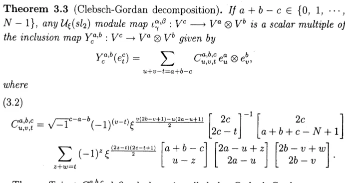
get the following.

Theorem 3.3 (Clebsch-Gordan decomposition).

_If

$a+b-c\in\{0,1,$ $\cdots$ ,

$N-1\}$, any $\mathcal{U}_{\xi}(sl_{2})$ module map $\iota_{\gamma}^{\alpha,\beta}$ : $V^{c}arrow V^{a}\otimes V^{b}$ is

a

scalar multiple

of

the inclusion map $Y_{c}^{a,b}:V^{c}arrow V^{a}\otimes V^{b}$ given by

$Y_{c}^{a,b}(e_{t}^{c})= \sum_{u+v-t=a+b-c}C_{u,v,t}^{a,b,c}e_{u}^{a}\otimes e_{v}^{b}$,

where

(3.2)

$C_{u,v,t}^{a,b,c}=\sqrt{-1}^{c-a-b}(-1)^{(v-t)}\xi^{\frac{v(2b-v+1)-u(2a-u+1)}{2}}\{\begin{array}{ll} 2c2c -t\end{array}\}\{\begin{array}{ll}2c a+b+c-N +1\end{array}\}$

$\sum_{z+w=t}(-1)^{z}\xi^{\frac{(2z-t)(2c-t+1)}{2}}\{\begin{array}{l}a+b-cu-z\end{array}\}$ $\{\begin{array}{l}2a-u+z2a-u\end{array}\}\{\begin{array}{l}2b-v+w2b-v\end{array}\}$ .

The coefficient $C_{u,v,t}^{a,b,c}$ defined above is called the Crebsch-Gordan quantum

coefficient

(CGQC). In order to get invariants of graphs, the operators $L_{a,b}^{c}$

and $R_{a,b}^{c}$ in Figure 1 must be equal, and

we

define $Y_{a,b}^{c}$ by $Y_{a,b}^{c}=L_{a,b}^{c}$. The

equality of $L_{a,b}^{c}$ and $R_{a,b}^{c}$

comes

from the following lemma.

$c$ $c$ $c$

$Y_{a,b}^{c}$ $L_{a,b}^{c}$ $R_{a,b}^{c}$

FIGURE 1. The first equality is the definition of $Y_{a,b}^{c}$, the second

is Lemma 3.4.

Lemma 3.4. It holds that

$C_{N-1-u,t,v}^{N-1-a,c,b}\xi^{-a(N-1)}\xi^{(N-1)u}=C_{t,N-1-v,u}^{c,N-1-b,a}\xi^{-(N-1-b)(N-1)}\xi^{(N-1)(N-1-v)}$.

Proposition

3.5. The

projection $Y_{a,b}^{c}:V^{a}\otimes V^{b}arrow V^{c}$ is given by

(3.3) $Y_{a,b}^{c}(e_{u}^{a}\otimes e_{v}^{b})=C_{N-1-v,N-1-u,N-1-t}^{N-1-b,N-1-a,N-1-c}(e_{t}^{c})$.

3.3.

The R-matrix. The R-matrix corresponding to the colored Alexander

invariant is given in [1], and is also used in [25]. The construction of the

representation of $\mathcal{U}_{\xi_{n}}(sl_{2})$ is

a

little bit different from that in [25], and

we

define $abR:V^{a}\otimes V^{b}arrow V^{b}\otimes V^{a}$

as

follows:

(3.4) $abR(e_{u}^{a}\otimes e_{v}^{b})=$

$\sum_{m\geq 0}\{m\}!\xi_{n}^{2(a-u)(b-v)-m(a-b-u+v)-\frac{m(m+1)}{2}}\{\begin{array}{l}uu-m\end{array}\}\{\begin{array}{l}2b-v2b-v-m\end{array}\}e_{v+m}^{b}\otimes e_{u-m}^{a}$.

We denote

_ab

$u$

$R^{h},t$ the coefficient of $R(e_{u}^{a}\otimes e_{v}^{b})$ with respect to $e_{h}^{b}\otimes e_{k}^{a}$.

Proposition 3.6. The morphism $abR$ given above is the R-matrix

of

the

non-integml representations, in other words, $abR$

satisfies

(3.5) $ab$$R\triangle(x)=\triangle(x)_{a}^{b}R$

as

mappings

_from

$V^{a}\otimes V^{b}$ to $V^{b}\otimes V^{a}$

for

any $x\in \mathcal{U}_{\xi}.(sl_{2})$, and

(3.6) $(_{b}^{c}R\otimes$ $id$_$)($$id$$\otimes_{a}^{c}R)(_{a}^{b}R\otimes$ $id$$)=($$id$$\otimes_{a}^{b}R)(_{a}^{c}R\otimes$ $id$$)($$id$ $\otimes_{b}^{c}R)$

as

mappings

_from

$V^{a}\otimes V^{b}\otimes V^{c}$ to $V^{c}\otimes V^{b}\otimes V^{a}$.

The R-matrix given by (3.4) is represented graphically

as

follows.

aklb

Rij _: $(_{a}^{b}R^{-1})_{kl}^{ij}$ :

$k$ $l$ $k$ $l$

3.4.

Invariants oftrivalent planar graphs. Let

now

$\Gamma$ be

a

framed oriented

connected trivalent graph in $S^{3}$ and let

us

fix

once

and for all a natural number

$N\geq 2$

as

well as a root $\xi=\exp(\frac{\pi\sqrt{-1}}{N})$.

Definition 3.7 (Coloring). A coloring

on

$\Gamma$ is

a

map col: _{$\{edges\}arrow \mathbb{C}\backslash \frac{1}{2}\mathbb{Z}$}

such that for each three uple of edges $e_{1},$ $e_{2},$ $e_{3}$ sharing a vertex $v$ (possibly

two edges coincinding) it holds:

$f_{v}(e_{1})+f_{v}(e_{2})+f_{v}(e_{3})\in\{0,1, \ldots N-1\}$,

Given an trivalent graph $\Gamma$ embedded in $S^{3}$ equipped with

an

orientation of

its edges, a framing and

a

coloring (such

a

datum will be from

now

on called

colored oriented graph),

we can

associate to it

a

complex number which

we

shall denote $\langle\Gamma$, col$\rangle_{N}$ by the following construction.

(1) Choose an edge $e_{0}$ of $\Gamma$ and cut $\Gamma$ open along $e_{0}$.

(2) Move by

an

isotopy $\Gamma$

so

to put it in a (1, 1)-tangle diagram and

so

that the two open strands initially contained in $e_{0}$

are

directed towards the bottom.

(3) Assigning $\cap$ operators to the maximal points, $\cup$ operators to the

min-imal points, R-matrices to the crossing points and the Crebsh-Gordan

operators $Y_{a}^{b,c}$ and $Y_{a,b}^{c}$ to the trivalent vertices as in [19], we associate

to the diagram $D$ of $\Gamma$ obtained in (3) an operator op$(D)$ : $V^{co1(eo)}arrow$

$V^{co1(e_{0})}$ and hence, by Schur

$s$ lemma, a scalar $\lambda(D)\in \mathbb{C}$.

(4) Define the scalar associated to $D$ as $i(D)=\lambda(D)\{\begin{array}{l}2col(e_{0})+N2col(e_{0})+1\end{array}\}$

Theorem 3.8. The scalar $i(D)$ is independent on all the choices

of

the above

construction and is

_therefore

an invariant $<\Gamma$, col $>_{N}\in \mathbb{C}$

of

the colored

ori-ented graph embedded in $S^{3}$.

The invariance under the Reidemeister

moves

is proved as usual quantum

invariants. The extra thing is to show the invariance under the choice of edge

$e_{0}$ to cut the graph open. The factor $[2co1(e_{0})+N2co1(e_{0})+1]^{-1}$ is added for this

purpose and the following lemma assures the invariance.

Lemma 3.9. Let $\theta(a, b, c)$ be a $\theta$-graph embedded in the standard way in the

plane, colored by $a,$ $b,$ $c \in \mathbb{C}\backslash \frac{1}{2}\mathbb{Z}$ and such that the edges colored by _$a,$$b$ have

the

same

source, while that colored by $c$ has

a

different

source.

Then, letting

$\theta_{a}(a, b, c)$ be the diagmm obtained by cutting open $\theta$ along the a-colored edge it holds that

(3.7) $\lambda(\theta_{a}(a, b, c))=\{\begin{array}{l}2a+N2a+1\end{array}\}$ ,

and so we get $i(\theta_{a}(a, b, c))=i(\theta_{b}(a, b, c))=1$.

This lemma

comes

from the following relation.

$\{\begin{array}{l}2a+N2a+1\end{array}\}=\sum_{t=0}^{N-1+c-b-a}C_{a+b-c+t,N-1-t,N-1}^{b,N-1-c,N-1-a}C_{t,N-1+c-a-b-t,0}^{c,N-1-b,a}$ .

$arrow$

FIGURE 2. On the left $\theta_{a}(a, b, c)$;

on

the right $\theta_{b}(a, b, c)$.

Lemma 3.10. For any pammeter $a,$ $b$ and

a

non-negative integer $c$,

we

have (3.8) $\sum_{s=0}^{c}q^{\pm(a+b-c+2)s}\{\begin{array}{l}a-sa-c\end{array}\}$ $\{\begin{array}{l}b+sb\end{array}\}=q^{\pm(b+1)c}\{\begin{array}{ll}a+b +1a+b-c +1\end{array}\}$

For generic $q$, this relation is true for the

case

that $a$ and $b$

are

non-negative

integers by (51) in [18]. The both sides of (3.8)

are

Laurent polynomials with

respect to the variable $q^{a},$ $q^{b}$, and they are equal for any positive integers $a$

and $b$. Therefore, these two polynomials

are

equal and the both sides of (3.8)

coinside for any $a$ and $b$ for generic

$q$. Then

we

can

specialize $q$ to the $2N$-th

root of unity and

we

get (3.8). The formula (3.7) implies that

$Y_{c}^{a,b}Y_{a,b}^{c}Y_{c}^{a,b}Y_{a,b}^{c}=\{\begin{array}{l}2c+N2c+1\end{array}\}Y_{c}^{a,b}Y_{a,b}^{c}$.

Hence, $\{\begin{array}{l}2c+N2c+l\end{array}\}Y_{c}^{a,b}Y_{a,b}^{c}$ is the identity

on

the subspace of $V^{a}\otimes V^{b}$

iso-morphic to $V^{c}$. Therefore, the decomposition of $V^{a}\otimes V^{b}$ is expressed by $Y_{c}^{a,b}$

and $Y_{a,b}^{c}$

as

follows.

(3.9) id $= \sum_{c;a+b-c=0,1,\cdots,n-1}\{\begin{array}{l}2_{C}+N2c+1\end{array}\}Y_{c}^{a,b}Y_{a,b}^{c}$.

Remark 3.11. Colored graphs include colored links, and the invariant defined

above is the colored Alexander invariant given in [1] and discussed in [12], [25].

Lemma 3.9 gives a new proof for the independence ofthe string to cut to make

a

(1, 1)-tangle. It is first proved in [1] by computation, and then refined in

[12] for

more

general

cases

theoretically. Comparing with the proof in [12], we

see

that $\{\begin{array}{l}2a+N2a+1\end{array}\}$ corresponds to $d(a)$ in Definition 2.3 of [12] expressing

4. $SL(2,$$\mathbb{C})$ QUANTUM $6j$-SYMBOLS

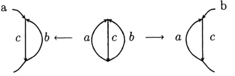
4.1. Construction. The quantum $6j$-symbol is defined by the relation in

Figure 3. The left diagram

means

that the composition of two inclusions

$V_{i}arrow V_{j_{12}}\otimes V_{j_{3}}$ and $V_{j_{12}}arrow V_{j_{1}}\otimes V_{j_{2}}$ and the right diagram

means

that the

composition of two inclusions $V_{j}arrow V_{j_{1}}\otimes V_{j_{23}}$ and $V_{j_{23}}arrow V_{j_{2}}\otimes V_{j_{3}}$ .

Let

$\iota_{l}:V_{j}arrow V_{j_{12}}\otimes V_{j_{3}}arrow(V_{j_{1}}\otimes V_{j_{2}})\otimes V_{j_{3}}$

$($resp.

$\iota_{r}$ : $V_{j}arrow V_{j_{1}}\otimes V_{j_{23}}arrow V_{j_{1}}\otimes(V_{j_{2}}\otimes V_{j_{3}}))$

be the inclusion corresponding to the left (resp. right) diagram. Then Figure

3

means

that

$\iota_{l}(v)=\sum_{j_{23}}\{\begin{array}{lll}j_{1} j_{2} j_{12}j_{3} j j_{23}\end{array}\} \iota_{r}(v)$

for $v\in V_{j}$. The quantum $6j$-symbol for non-integral highest weight represen-tations

are

given

as

follows.

$= \sum_{j_{23}}\{\begin{array}{l}j_{1}j_{3}\end{array}$

$j$

$j_{2}$

$j$

$j$

FIGURE 3. The quantum $6j$-symbol

Theorem 4.1. For$a,$ $b,$ _$\cdots,$ $f$ satisfying$a+b-e,$$a+f-c,$ $b+d-f,$ $d+e-c\in \mathbb{Z}$,

(4.1) $\{\begin{array}{lll}a b ed c f\end{array}\}=$

$(-1)^{N-1+B_{afc}} \{\begin{array}{l}2f+N2f+1\end{array}\}\frac{\{B_{dec}\}!\{B_{abe}\}!}{\{B_{bdf}\}!\{B_{afc}\}!}\{\begin{array}{lll} 2e A_{abe} +1- N\end{array}\} \{\begin{array}{l}2eB_{ecd}\end{array}\}$

$z= \max(0,-B_{bdf}+B_{dec}),B_{afc})\sum^{\min(B_{dec}}(-1)^{z}\{\begin{array}{ll}A_{afc} +12c+z +1\end{array}\} \{\begin{array}{l}B_{acf}+zB_{acf}\end{array}\}\{\begin{array}{l}B_{bfd}+B_{dec}-zB_{bfd}\end{array}\}\{\begin{array}{l}B_{dce}+zB_{dfb}\end{array}\}$ ,

where

Remark. Such $6j$-symbol is already given in [10] for the

case

that $n$ is odd.

This theorem is proved

as

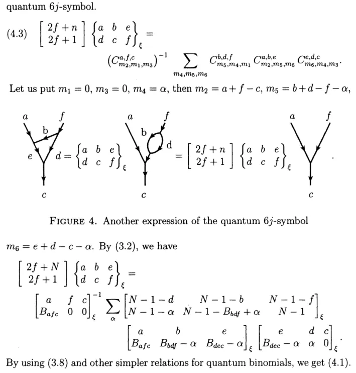
follows. Using the value of the theta graph (3.7),

we have the relation in Figure 3. This gives the following expression of the

quantum $6j$-symbol.

(4.3) $[2f:n2f1]\{\begin{array}{lll}a b ed c f\end{array}\}=$

$(C_{mm,m}^{a,f,c_{1}}2,3)^{-1} \sum_{m_{4},m_{5},m6}C_{m_{5},m_{4}}^{b,d,f},{}_{m_{1}}C_{m_{2},m}^{a,b,e_{5}},{}_{m_{6}}C_{m_{6},m,m3}^{e,d,c_{4}}$ .

Let

us

put $m_{1}=0,$ $m_{3}=0,$ $m_{4}=\alpha$, then $m_{2}=a+f-c,$ $m_{5}=b+d-f-\alpha$,

$b$

$c$

$c$ $c$

$\{\begin{array}{l}a bdc\end{array}$

$c$

FIGURE 4. Another expression of the quantum $6j$-symbol

$m_{6}=e+d-c-\alpha$_. By _(3.2), we have

$\{\begin{array}{l}2f+N2f+1\end{array}\}\{\begin{array}{lll}a b ed c f\end{array}\}=$

$\{\begin{array}{lll}a f cB_{afc} 0 0\end{array}\}\sum_{\alpha}\{\begin{array}{lllllllll}N -1- d N-l- b N -1- fN -1- \alpha N -1- B_{bdf}+\alpha N-1 \end{array}\}$

$\{\begin{array}{lll}a b eB_{afc} B_{bdf}-\alpha B_{dec}-\alpha\end{array}\}\{\begin{array}{lll}e d cB_{dec}-\alpha \alpha 0\end{array}\}$

By using (3.8) and other simpler relations for quantum binomials,

we

get (4.1).

4.2. Relations among the quantum $6j$-symbols. From the definition of

$SL(2, \mathbb{C})$ quantum $6j$-symbols, they satisfy the following relations.

Orthogonarity relation:

FIGURE 5. Colored oriented tetrahedral graph

Pentagon relation:

$\sum_{h}\{\begin{array}{lll}a b fg c h\end{array}\} \{\begin{array}{lll}a h ge d i\end{array}\}\{\begin{array}{lll}b c hd i j\end{array}\}= \{\begin{array}{lll}f c gd e j\end{array}\}\{\begin{array}{lll}a b fj e i\end{array}\}$

4.3.

Values of tetrahedra. The value $\{\begin{array}{lll}a b ed c f\end{array}\}$ of the colored oriented

graph corresponding to a tetrahedron in Figure 5 is given as follows.

Theorem 4.2. Assume that

none

_of

the colors $a,$ $b,$ $c,$ $d,$ $e,$ $f$ is a half-integer

and they satisfy the admissibility condition

_for

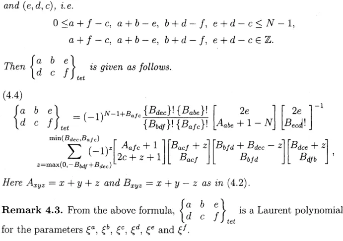
triples $(a, f, c),$ $(a, b, e),$ $(b, d, f)$

and $(e, d, c),$ $i.e$.

$0\leq a+f-c,$ _{$a+b-e,$ $b+d-f,$} $e+d-c\leq N-1$,

$a+f-c,$

$a+b-e,$ $b+d-f,$ $e+d-c\in \mathbb{Z}$.

Then $\{\begin{array}{lll}a b ed c f\end{array}\}$ is given

as

follows.

(4.4)

$\{\begin{array}{lll}a b ed c f\end{array}\}=(-1)^{N-1+B_{afc}}\frac{\{B_{dec}\}!\{B_{abe}\}}{\{B_{bdf}\}!\{B_{afc}\}}!\{\begin{array}{lll} 2e A_{abe} +1- N\end{array}\} \{\begin{array}{ll}2e B_{ec}d !\end{array}\}$

$z= \max(0,-B_{bdf}+B_{dec}),B_{afc})\sum^{\min(B_{dec}}(-1)^{z}[_{2c+z+1}A_{afc}+1]\{\begin{array}{l}B_{acf}+zB_{acf}\end{array}\}\{\begin{array}{l}B_{bfd}+B_{dec}-zB_{bfd}\end{array}\}\{\begin{array}{l}B_{dce}+zB_{dfb}\end{array}\}$ ,

Here $A_{xyz}=x+y+z$ and $B_{xyz}=x+y-z$ as in (4.2).

Remark 4.3. From the above formula, $\{\begin{array}{lll}a b ed c f\end{array}\}$ is a Laurent polynomial

for the parameters $\xi^{a},$ $\xi^{b},$ $\xi^{c},$ $\xi^{d},$ $\xi^{e}$ and $\xi^{f}$.

4.4. Relations of the values of the tetrahedra. From the relations of the

Orthogonal relation:

$\{\begin{array}{l}f+Nf+1\end{array}\}\{\begin{array}{l}g+N+g1\end{array}\}\{\begin{array}{l}ad\end{array}$

Pentagon relation:

$cb$ _{$fetet\{\begin{array}{lll}d b fa c g\end{array}\}=\delta_{eg}$},

$\sum_{h}\{\begin{array}{l}h+Nh+1\end{array}\}\{\begin{array}{lll}a b fg c h\end{array}\} \{\begin{array}{lll}a h ge d i\end{array}\}\{\begin{array}{lll}b c hd i j\end{array}\}=$

$\{\begin{array}{lll}f c gd e j\end{array}\}\{\begin{array}{lll}a b fj e i\end{array}\}$

Symmetry: Since the change of the orientation of an edge colored by $i$

corresponds to the change ofthe color $i$ to $\overline{i}=N-1-i$,

we

have the following

symmetry.

(4.5) $\{\begin{array}{lll}a b ed c f\end{array}\}=\{\begin{array}{ll}b\overline{e}\overline{a} fc d\end{array}\}= \{_{b}^{c}\overline{fe}\frac{a}{d}\}_{tet}=$

$\{\begin{array}{lll}d e c\overline{a}f b\end{array}\}=\{\frac{e}{f}ad\frac{c}{b}\}_{tet}=\{\begin{array}{ll}f\overline{b} ace d\end{array}\}$

4.5. Volume of

a

truncated tetrahedron. Let $T$ be the truncated

tetra-hedron with dihedral angles $\theta_{a},$ $\theta_{b},$ $\theta_{c},$ $\theta_{d},$ $\theta_{e},$ $\theta_{f}$.

$\ldots$ , $f_{N}=\{$

Theorem 4.4. Let $T$ be the truncated tetrahedmn with oriented labeled edges

as

in Fignre 5, and let $0<\theta_{a},$ $\theta_{b},$ $\theta_{c},$ $\theta_{d},$ $\theta_{ez}\theta_{f}<\pi$ be the dihedral angles at

the edges.

_If

$\theta_{i},$ $\theta_{j},$ $\theta_{k}$

are

three dihedml angles meeting at the

same

vertex,

then they satisfy $\theta_{i}+\theta_{j}+\theta_{k}<\pi$ since $T$ is a truncated tetmhedmn. Put

$a_{N}= \lfloor(1-\frac{\theta_{a}}{\pi})\frac{N-1}{2}\rfloor$ , $(1- \frac{\theta_{f}}{\pi})\frac{N-1}{2}\rfloor$ ,

and $\overline{a}_{N}=N-1-a_{N},$ $\cdots,$ $\overline{f}_{N}=N-1-f_{N}$. Using these pammeters, the

volume

_of

$T$ is given as

follows.

$Vol(T)=\lim_{Narrow\infty}\frac{\pi}{2N}\log(\{\begin{array}{lll}a_{N} b_{N} e_{N}d_{N} c_{N} f_{N}\end{array}\} \{\begin{array}{lll}\overline{a}_{N} \overline{b}_{N} \overline{e}_{N}\overline{d}_{N} \overline{c}_{N}\overline{f}_{N} \end{array}\})$ .

Remark 4.5. $\{\begin{array}{lll}a_{N} b_{N} e_{N}d_{N} c_{N} f_{N}\end{array}\}$ isdefined for tetrahedron withoriented edges,

and it is not symmetric with respect to the natural symmetry of the

tetrahe-dron. However, the limit ofthe above

sum

becomes symmetric.

The above theorem is proved by using the Schl\"afli

differential

equality and

Question

4.6.

In [11],

a

_3-manifold

invariant is constructed

_from

such

6j-symbols. Explain the relation between this invariant and the hyperbolic volume

of

the

_3-manifold.

REFERENCES

1. Y. Akutsu, T. Deguchi and T. Ohtsuki, Invariants of colored links. J. Knot Theory

Ramifications 1 (1992), 161-184.

2. Q. Chen, S. Kuppum and P. Srinivasan, On the relation between the WRT invariant

and the Hennings invariant, Math. Proc. Camb. Phil. Soc. 146 (2009), 151-163.

3. Y. Choand H. Kim, Onthe volumeformulaforhyperbolic tetrahedra. Discrete Comput.

Geom. 22 (1999), 347-366.

4. J. Cho and J. Murakami, Some limits of the colored Alexander invariant of the

figure-eight knot and the volume of hyperbolic orbifolds. J. Knot Theory

_{Ramifications}

18

(2009), 1271-1286.

5. F. Costantino, Coloured Jones invariants of links and the volume conjecture. J. Lond.

Math. Soc. (2) 76 (2007), 1-15.

6. F. Costantino, $6j$-symbols, hyperbolic structures and the volume conjecture. Geom.

Topol. 11 (2007), 1831-1854.

7. F. _{Costantino, Integrality of Kauffman brackets of trivalent graphs. preprint,}

arXiv:0908.0542.

8. F. Costantino and J. Murakami On SL(2, C) quantum $6j$-symbol and its relation to the

hyperbolic volume. arXiv:l

_005.4277

9. B. L. Feigin, A.M. Gainutdinov, A. M. Semikhatov, and I. Yu. Tipunin, Modular group

representations and _fusion in logarithmic _conformal

_field

theories and in the quantum

group center, Comm. Math. Phys. 265 (2006), no. 1, 47-93.

10. N. Geer and B. Patureau-Mirand. Polynomial $6j$-symbols and states sums. preprint,

arXiv:0911.1353.

11. N. Geer, B. Patureau-Mirand and V. Turaev Modified $6j$-Symbols and 3-Manifold

In-variants. preprint,

_{arXiv:0910.1624.}

12. N. Geer and N. Reshetikhin, On invariants of graphs related to quantum $sl_{2}$ at root of

unity. Lett. Math. Phys. 88 (2009), 321-331.

13. S. Gukov, Three-dimensional quantum gravity, Chern-Simons theory, and the

A-polynomial. Comm. Math. Phys. 255 (2005), 577-627.

14. R. Hartley, The Conway potential function for links. Comment. Math. Helv. 58 (1983),

365-378.

15. M. Hennings, Invariantsof linksand3-manifoldsobtained fromHopfalgebras. J. London

Math. Soc. (2) 54 (1996), 594-624.

16. R. Kashaev, A link invariant from quantum dilogarithm, Modem Phys. Lett. A 10

(1995), no. 19, 1409-1418.

17. R. Kashaev, The hyperbolic volumeofknots fromthe quantumdilogarithm. Lett. Math.

18. A.N. Kirillov, Clebsch-Gordanquantum coefficients. J. SovietMath. 53 (1991), 264-276.

19. A.N. Kirillov and N. Yu. Reshetikhin, Representations of the algebra $\mathcal{U}_{q}(sl_{2}),$

q-orthogonal polynomialsand invariants of links. In

_{Infinite-dimensional}

Lie algebras and

groups (Luminy-Marseille, 1988), Adv. Ser. Math. Phys. 7, World Scientific, Teaneck

1989, 285-339.

20. J. Milnor, The Schl\"afli differential equality, John Milnor Collected Papers Volume 1

Geometry, 281-295, Pblish or Perish, Houston, Texas.

21. H. Murakami, optimistic calculations about the Witten-Reshetikhin-Turaev invariants

ofclosed three-manifolds obtained fromthe figure-eightknot by integral Dehn surgeries.

Recent progress towards the volume conjecture (Kyoto, 2000). Surikaisekikenkyusho

Kokyuroku 1172 (2000), 70-79.

22. H. Murakami andJ. Murakami, The colored Jones polynomials and the simplicial volume

ofa knot. Acta Math. 186 (2001), 85-104.

23. H. Murakami, J. Murakami, M. Okamoto, T. Takata, Y. Yokota, Kashaevs conjecture

and the Chern-Simons invariants of knots and links. Expenment. Math. 11 (2002),

427-435.

24. H. Murakami and Y. Yokota, The colored Jones polynomials of the figure-eight knot

and its Dehn surgery spaces. J. Reine Angew. Math. 607 (2007), 47-68.

25. J. Murakami, Colored Alexander invariants and cone-manifolds. Osaka J. Math. 45

(2008), 541-564.

26. J. Murakami and K. Nagatomo, Logarithmic knot invariants arisilig from restricted

quantum groups. Intemat. J. Math. 19 (2008), 1203-1213.

27. J. Murakami and A. Ushijima, A volume formula for hyperbolic tetrahedra in terms of

edge lengths. J. Geom. 83 (2005), 153-163.

28. J. Murakami and M. Yano, On the volume of a hyperbolic and spherical tetrahedron.

Comm. Anal. Geom. 13 (2005), 379-400.

29. N.Yu. Reshetikhin and V. G. Tuaev, Invariants of3-manifolds via link polynomials and

quantum groups. Invent. Math. 103 (1991), 547-597.

30. V.G. Turaev and O. Ya. Viro, State sum invariants of 3-manifolds and quantum

6j-symbols. Topology 31 (1992), 865-902.

31. A. Ushijima, A volume formulafor generalised hyperbolic tetrahedra. In Non-Euclidean

geometries, Math. Appl. (N. Y.) 581, Springer, New York 2006, 249-265.

32. O. Viro, Quantum relatives of the Alexander polynomial. St. Petersburg Math. J. 18

(2007), 391-457.

33. Y. Yokota, On the volume conjecture for hyperbolic knots, arXiv:math/0009l\’o5.

Jun Murakami

Department of Mathematics

Faculty ofScience and Engineering

Waseda University

3-4-1 Ohkubo, Shinjuku-ku

Tokyo 169-8555, JAPAN