JAIST Repository: 感情音声変換のためのARX-LFモデルに基づいて感情音声の分析

(1)

JAIST Repository

https://dspace.jaist.ac.jp/

Title 感情音声変換のためのARX-LFモデルに基づいて感情音

声の分析 Author(s) Li, Yongwei Citation

Issue Date 2014-03

Type Thesis or Dissertation Text version author

URL http://hdl.handle.net/10119/12020 Rights

(2)

Analysis of emotional speech based on ARX-LF

model for emotional speech conversion

By Yongwei Li

A thesis submitted to

School of Information Science,

Japan Advanced Institute of Science and Technology,

in partial fulfillment of the requirements

for the degree of

Master of Information Science

Graduate Program in Information Science

Written under the direction of

Professor Masato Akagi

(3)

Analysis of emotional speech based on ARX-LF

model for emotional speech conversion

By Yongwei Li (1210059)

A thesis submitted to

School of Information Science,

Japan Advanced Institute of Science and Technology,

in partial fulfillment of the requirements

for the degree of

Master of Information Science

Graduate Program in Information Science

Written under the direction of

Professor Masato Akagi

and approved by

Professor Masato Akagi

Professor Jianwu Dang

Associate Professor Masashi Unoki

February, 2014 (Submitted)

(4)

List of Figures

1.1 GMM method . . . 7

1.2 Diﬀerent emotional degrees of human speech . . . 8

1.3 Three-layer moedl method . . . 9

1.4 Speech production mechanism . . . 10

1.5 The concept of research . . . 12

2.1 Source-ﬁlter theory . . . 13

2.2 LF model that functionally mimics derivative of glottal ﬂow . . . 14

2.3 ARX model . . . 15

3.1 Speech signal waveform . . . 17

3.2 Example of GCI extraction on a voiced segment: (a) the speech signal, (b) its corresponding mean-based signal, (c) the LP residual with the detected GCIs. . . 18

3.3 Example of GOI extraction on a voiced segment: (a) speech signal (b) LP residual with the detected GCIs are expressed by red circle , (c) HE of LP residual with the detected GOIs are expressed by green asterisk. . . 20

3.4 Flowchart of ARX-LF model with accurate GCI and GOI . . . 21

3.5 Example of /a/ on neutral speech: (a) the waveform of LF model, (b) the vocal tract imformation, (c) the LP spectrum envelope, (d) the error of our result, (e) the error of previous result. . . 23

3.6 Example of /a/ on joy speech: (a) the waveform of LF model, (b) the vocal tract imformation, (c) the LP spectrum envelope, (d) the error of our result, (e) the error of previous result. . . 24

3.7 Example of /a/ on sad speech: (a) the waveform of LF model, (b) the vocal tract imformation, (c) the LP spectrum envelope, (d) the error of our result, (e) the error of previous result. . . 25

3.8 Example of /a/ on anger speech: (a) the waveform of LF model, (b) the vocal tract imformation, (c) the LP spectrum envelope, (d) the error of our result, (e) the error of previous result. . . 26

4.1 /a/ of “a t/a/ ra shi i me-ru ga to do i te i ma su”, the glottal waveform derivative and glottal waveform in neutral, joy, sad and anger speech. . . . 30

4.2 example: /a/ of “a t/a/ ra shi i me-ru ga to do i te i ma su”, glottal source spectral. . . 31

(7)

4.3 /a/ of “ma chi /a/ wa se ha a o ya ma ra shi i N de su”, the glottal waveform derivative and glottal waveform in neutral, joy, sad and anger speech.the glottal waveform diﬀerentive and glottal waveform in neutral, joy, sad and

anger speech. . . 32

4.4 /a/ of “i ra n/a/ i me-ru ga a Q ta ra su te te ku da sa i”, the glottal

waveform derivative and glottal waveform in neutral, joy, sad and anger

speech . . . 33

4.5 /a/ of “so N n/a/ no gu ru i me i shi N de su yo”, the glottal waveform

derivative and glottal waveform in neutral, joy, sad and anger speech. . . . 34

4.6 /a/ of “Te ga mi g/a/ to do i ta ha zu de su”, the glottal waveform derivative

and glottal waveform in neutral, joy, sad and anger speech. . . 35

4.7 /a/ of “Ha n/a/ bi wo mi ru no ni go za ga i ri ma su ka”, the glottal

waveform derivative and glottal waveform in neutral, joy, sad and anger

speecp. . . 36

(8)

List of Tables

4.1 Parameters of the LF model . . . 30

(9)

Chapter 1 Introduction

1.1 Motivation

Communication is one of the most important activities of human being. Speech is one of most important ways to communicate with each other. In speech communication, not only the linguistic meaning, but also non-linguistic imformation is transmitted, such as age, gender and emotion. The emotion can make our communication more interesting and expressive. Many researchers want to get human-like speech(expressive speech) for some applications. Thus, emotional speech synthesis and emotional speech conversion are hot topics in the area of speech signal processing.

Nowdays, speech synthesis techniques have been well developed; e.g., text reading sys-tem, speech-oriented guidance syssys-tem, and syntheszing singing voice. However, in these system only the linguistic information is synthesized, and they cannot handle human emo-tion. So emotional speech conversion is widely studied based on neutral speech in recent years. Comparison of neutral speech signals and emotional ones is an essential step in emotional speech conversion processing. Many approaches were mainly based on analysis of acoustic features and transformation from one acoustic features set to another acoustic feature set using GMM method. However, these methods overlooked the human speech system (speech perception and speech production). The converted emotional degrees of human are limited by traditional methods.

In order to solve those problems, we come back to consider human speech production mechanisms and speech perception mechanisms. A three-layer perceptual model were well-constructed by Huang and Akagi [9]. Thus, we focus on speech production mechanisms in this research, it is well known that the vocal fold as a glottal source plays an important role in speech production mechanisms. Thus, analysis of glottal source wave of emotional speech is an important work for emotional speech conversion. The analysis results can be further used for emotional speech conversion. The converted speech can be used in many speech applications.

(10)

1.2 Background

Up to now, a rather large number of research works are statistics-based method.

1.2.1 GMM method

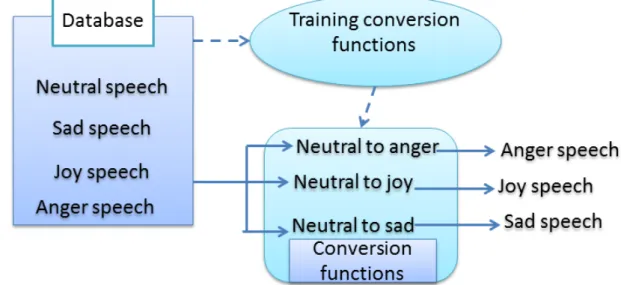
Figure 1.1: GMM method

Gausian Mixture Model (GMM) is a statistics-based method widely used for emotional speech conversion such as [1] [2] [3] [4] [5] [6]. One example, Kawanami et al. used GMM for emotional speech conversion [7], as shown in the Figure 1.1. In this method, preparing a large database is the frist step. In the second step, and the mel cepstrum coeﬃcient is selected for GMM training to ﬁnd out the training conversion functions. Finally, emotional speech is converted from neutral speech by using training conversion fuctions.

1.2.2 Problems of GMM method

It is well known that an emotional state have diﬀerent degree of intensity which may change over time depending on the situtation from low to high degree. In other words, a large number of emotional degrees in the real-life which can be described in Activation and Valence domain as shown in Figure 1.2.

A large database is needed in GMM method, however, the database including all emo-tional degrees is diﬃcult. In a few words, GMM method can only convert emoemo-tional speech inside of database and converting a lot of emotional degrees is diﬀcult.

(11)

Figure 1.2: Diﬀerent emotional degrees of human speech

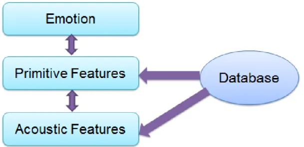
1.2.3 Three-layer model

Cahn [8] first consider human perceptual ability and proposed two-layer perceptual model. However, human ability to perceive emotions from the speech was not directly based on acustics. Thus, Huang and akagi proposed a three-layer perceptual model to simulate hu-man ability to perceive emotions from speech. The three-layer perceptual model consists of emotion layer, semantic primitives layer and acoustic features layer [9]. The three-layer model is shown in Figure 1.2. In this method, first step is to analyze acoustic feature char-acteristics and semantic primitives from different emotional speech signals. the second step is to findout the relationship between each layer and construct rules between each layer. Finally, in order to evaluate the relationship, the emotional speech is converted from neutral speech by controlling acoustic features using Speech Transformation and Representation using Adaptive Interpolation of weiGHTed spectrum (STRIGHT) [10].

1.2.4 Problems of three layer model

For three-layer model, the main work is to simulate human perceptual ability. The speech production mechanism was not fully considered although speech production mechanism is very important in emotional speech production.

In order to convert a lot of emotional degrees like human as much as possible. In analysis part, we need come back to consider the analysis of origin of human speech production for emotional speech conversion.

(12)

Figure 1.3: Three-layer moedl method

1.3 Speech production mechanism

The speech production mechanism consists three process: respiration, phonation and articulation [11]. A simple speech production process is shown in Figure 1.3.

Respiration is a physical process of gas exchange between an organism and its envi-ronment involving four steps (ventilation, distribution, perfusion and diffusion) and two processes (inspiration and expiration). Respiration can be described as the mechanical process of air flowing into and out of lungs on the principle of boyle’s law, stating that, as the volume of container increases, the air pressure will decrease. This relatively low pressure will cause air to enter the container until the pressure is equalized. During in-spiration of air, the diaphragm contracts and the lungs expand drawn by pleurae through surface tension and low pressure. When the lungs expand, air pressure becomes low com-pared to atmospheric pressure and air will flow form the area of high pressure to fill the lungs. Forced inspiration for speech uses accessory muscles to elevate the rib cage and enlarge the thoracic cavity in the vertical and lateral dimensions. During forced expira-tion for speech. muscles of the trunk and abdomen reduce the size of the thoracic cavity by compressing the abdomen or pulling the rib cage down forcing air out of the lungs.

Phonation is the production of a periodic sound wave by vibration of the vocal folds. Airflow form the lungs, as well as laryngeal muscle contraction, causes movement of the vocal folds. It is the properties of tension and elasticity that allow the vocal folfs to be stretched, bunched, brought together and separated. During prephonation, the vocal folds move from the abducted to adducted position. Subglottal pressure builds and air flow forces the folds apart, inferiorly to superiorly to superiorly. If the volume of airflow

(13)

Figure 1.4: Speech production mechanism

is constant, the velocity of the ﬂow will increase at the area of constriction and cause a decrease in pressure below once distributed. This negative pressure will pull the initially blow open ﬂods back together again. The cycle repeats until the vocal folds are abducted to inhibit phonation or to take a breath.

Articulation is the third process of speech production, mobile and immobile structures of the face (articulators) adjust the shape of the mouth, pharynx and nasal cavities (vocal tract) as the vocal fold vibration sound passes through producing varing resonant frequencies.

1.3.1 Glottal source model

The vocal fold plays an important role in the physical aspects of speech production mech-anism. Glottal source estimation is an important topic in speech signal processing, and can be used in many areas, such as speech conversion, speech recognition, speech enhance-ment and speech synthesis. Thus, many functional glottal source models are studied to mimic vocal fold vibration.

A classic glottal source analysis method: Linear Prediction (LP) analysis, a golttal source model is simply assumed as series of pulses for voiced sounds or white noise signals for unvoiced sounds. This oversimpliﬁed glottal source model often suﬀers from inadequate

(14)

representation of glottal source characteristics.

On the other hand, many glottal source models for estimating the parameters from speech signals have been proposed such as Rosenberg-Klatt (RK model) [12] and Liljencrant-Fant (LF) model [13, 14]. However, the parameters of these models were mainly estimated manually by researchers [12, 15]. The manual procedure causes a serious problem when analyzing a large number of speech data.

In order to solve the problem of manual operations in estimating glottal source pa-rameters, an automatic method has been proposed by Alku based on pitch-synchronous iterative adaptive inverse filtering [16, 17], the glottal source waveform is obtained by canceling the effects of the vocal tract and lip radiation by inverse filtering. However, this method can not explicitly separate glottal source and vocal tract information from speech signals.

To solve this problem, an Auto-Regressive eXogenous (ARX) model combined with the RK model was proposed by Ding, Kasuya and Adachi [18]. It is well known that the information of frequency domain is important in speech signal processing. Michael et al. shows that the return phase of glottal source has strong relationship with frequency energy [19]. The shorter return phase is, the larger frequency energy is. However, the return phase cannot be represented by the RK model. The return phase can be obtained by LF model. Thus, an ARX model combined with the LF model was proposed by Vincent et al. [20, 21]. The ARX-LF model is widely used for estimating glottal source parameters in recent years. For example, the glottal source parameters of singing signals is estimated by Motoda and Akagi based on the ARX-LF model [22].

In case of glottal source analysis of emotional speech, the parameters of glottal opening instant (GOI) are used as the start point of each period of LF model and glottal close instant (GCI) are used as the initial parameters of each period of LF model. Since the period of joy and anger speech is very short, enven small mistake may causes big error of analyzed results. However, the parameters of GOI and GCI are undervalued in the current ARX-LF model-based methods such as [22].

1.4 Purpose of this research

The three-layer model used for emotional speech recognition by Elbarougy [23], the results show that three-layer model is better than two-layer model. Thus, the three-layer model is more suitable for emotional speech conversion. The concept of this research is shown in Figure 1.4. The Figure contains two parts: the left part is three-layer perceptual model and the right part is main work of this research. Most of previous methods focus on analysis acoustic features without consider human speech system for emotional speech conversion. The emotional styles are limited by those methods.

In this paper, we focus on speech production mechanisms. The purpose of this research is to analyze glottal source wave of emotional speech for emotional speech conversion. The ARX-LF model is used for mimicking speech procuction mechanisms. In order to accurate estimation of glottal source wave of emotional speech, a suitable analysis approach is proposed. The diﬀerent glottal source wave of diﬀerent emotional speech were obtained.

(15)

Figure 1.5: The concept of research

The results are expected to be used to convert emotional speech with more emotional styles.

1.5 Organization of the thesis

The rest of the thesis is organised as follows:

• Chapter2 introduces the ARX model and the LF model. Since the ARX model and the LF model are the main tool for analyzing glottal source wave of emotional speech.

• Chapter3 describes our approach for analysis glottal source wave of emotional speech. In this chapter, we also discuss about the results of previous approach and the results of our approach. The results show that our approach is more suitable for analysis glottal source wave of emotional speech.

• Chapter4 focus on experiment, some speech signals are selected from database. The diﬀerent glottal source wave of diﬀerent emotional speech is obtained in this chapter.

(16)

Chapter 2 ARX-LF model

2.1 Source-filter theory of speech production

Acoustic speech output in humans and many nonhuman species is commonly considered to result from a combination of a source of sound energy(e.g. the largnx) modulated by a transfer function determined by the shape of the supralaryngeal vocal tract. This combination results in a shaped spectrum with broadband energy peaks. This model is often referred to as the “ source-ﬁlter theory of speech production” [24] and shown in Figure 2.1.

Figure 2.1: Source-ﬁlter theory

The source-filter theory describes speech production as a two stage process involving the generation of a sound source, with its own spectral shape and spectral finbe structure, which is then shaped or filtered by the resonant properties of the vocal tract.

Muller [25] noticed that the sound that came directly from the larynx diﬀered from the sounds of human speech. Speechlike quality could be achieved only when he placed over the vibrating cords a tube whose length was roughly equal to the length of the airways that normally intervene between the larynx and a person’s lips. The source of acoustic energy is at the largnx-the supralarygeal vocal tract serves as a variable acoustic ﬁlter whose shape determines the phonetic quality of the sound [26]

(17)

2.2 ARX-LF model

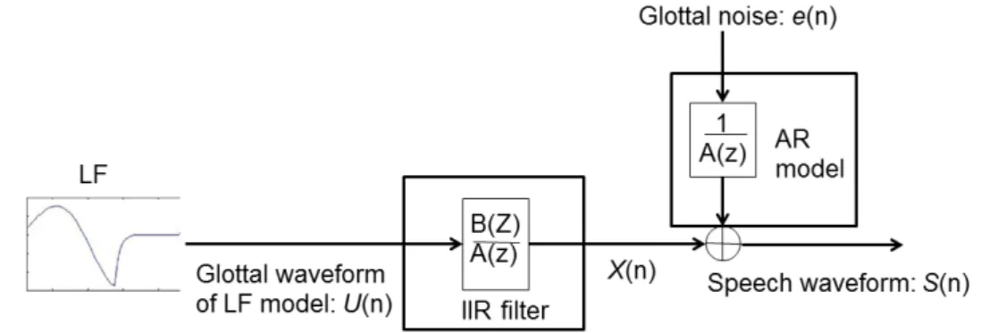
A common approach in speech processing is to represent the speech production mecha-nisms by means of a source-filter model. In such representation, the source component is refered to as the glottal flow derivative (GFD) [27], which incorporates the derivative effect due to the lips radiation to the signal observed at the glottis. A reasonable approx-mation of the GFD can be obtained through the LF model and the ARX model plays the vocal tract filter.

2.2.1 LF model

The LF model has ﬁve parameters used for representing the GFD. The ﬁve parameters

are four time points Tp, Te, Ta, T0, and one amplitude parameter Ee. If the start point

of the cycle is set to 0, and the end of the cycle is T0, where Tp is the phase of maximum

open of glottis, Te is the open phase of glottis (glottal close instant), Ta is the return

phase, Ee is the amplitude of glottal close instant and T0 is the period of vibration of the

vocal fold. the time domain LF model can be constructed by the equation 2.1, u(t) =

{

E1eatsin (wt) 0≤ t ≤ Te

−E2[e−b(t−Te)− e−b(T0−Te)] Te ≤ t ≤ T0

(2.1)

in which the parameters a, b and w are implicitly related to Tp, Te, Ta. A typical LF

waveform is depicted on Figure 2.2.

(18)

2.2.2 ARX model

The ARX model can simulate vocal tract. Speech production process can be modeled as a time-varying IIR system as follows:

s(n) +

p

∑

i=1

ai(n)s(n− i) = b0(n)u(n) + e(n) (2.2)

where s(n) is observed speech signal and u(n) is the glottal waveform (The LF waveform)

at time n, ai and b0 are time-varying coefficients of filter, p is filter order, and e(n) is the

equation error.

Figure 2.3: ARX model

The output signal of the LF model acts as an input signal u(n) to the vocal tract filter. Eq.(2) is called ARX model, as illustrated in Figure. 2.3. Input signal u(n) to the IIR filter is the glottal waveform, which is approximated by the LF model. We use the ARX model to represent the vocal tract filter. In this model, e(n) as a glottal noise in the speech production and its power in the voiced sound is obtained from the equation error. The vocal tract transfer function is defined as follows:

H(z) = B(z) A(z) =

1

1 + a1z−1+ ... + apz−p

(2.3) Input signal u(n) to the IIR ﬁlter is the glottal waveform which is approximated by the LF model. The out put signal x(n) plays a role in determining harmonic components in voiced sounds. In this way, we use the ARX model to represent the vocal tract ﬁlter.

(19)

Chapter 3 Implement ARX-LF model

The ARX-LF model can mimic speech production process, LF model is used to simulate the glottal source and the ARX model is used to simulate the vocal tract ﬂiter. In other words, the parameters of LF model and the parameters of ARX model can be estimated at the same time from speech signals. Since the purpose of this research is analysis of glottal source wave of emotional speech, we focus on LF model.

In order to implement ARX-LF model, the parameters of glottal opening instant (GOI) and the parameters of glottal close instant (GCI) must be obtained in advance. The parameters of GOI are used as the start point of each period of LF model and the GCI are used as the initial parameters of each period of LF model. The accuracy of estimated GOI and GCI aﬀects the results of LF model. Especially, in case of emotional speech. Since the period of joy and anger speech is very short, enven small mistake may causes big error of analyzed results.

3.1 Previous approach

Glottal source parameters of singing estimated by Motoda and Akagi based on the ARX-LF model. The GCI are considered to the negative maximum point of speech signal waveform. A part of speech signal waveform was cut and shown in Figure 3.1. The red circle is considered GCI as a input parameter of LF model in [22].

For the GOI, they assume candidates for the starting point be in a defined scope in the first period. For all the candidates, the mean-square equation error (MSEE) is calculated. The candidate with the least MSEE is regarded as the best strating point in the first period. From the second period on, the starting point of each period is set to a position in a distance of the fundamental period from the previous starting point.

When the GCI and GOI are obtained, the GCI and GOI are as the input parameters go to ARX-LF model. Then the glottal source wave are estimated by ARX-LF model.

(20)

0.01 0.02 0.03 0.04 0.05 0.06 0.07 0.08 -0.3 -0.2 -0.1 0 0.1 0.2 0.3 Time(s) Amplitude

Figure 3.1: Speech signal waveform

3.2 Proposed approach

GCI and GOI are important parameters for estimating the glottal source wave of emo-tional speech. In our approach, The mean-based signal method is selected for estimating GCI parameters [28, 29], and GOI parameter is estimated from the Hilbert envelop of LP residual [30].

3.2.1 Estimation of GCI

Estimation of GCI consists of two successive steps. During the ﬁrst step, a mean-based signal is computed, allowing the determination of short intervals where GCIs are expected to occur. As for the second step, it consits of a reﬁnement of the accurate locations from the LP residual signal.

The ﬁrst step, we focus analysis on a mean-based signal. If s(n) denotes the speech waveform, the mean-based signal y(n) is computed as:

y(n) = 1 2N + 1 N ∑ m=−N w(m)s(n + m) (3.1)

where w(m) is a windowing function of length 2N+1. In this case, we used a Blackman

(21)

0 0.02 0.04 0.06 0.08 0.1 0.12 −0.5 0 0.5 (a) Time [s] Amplitude 0 0.02 0.04 0.06 0.08 0.1 0.12 −1 0 1 (b) Time [s] Amplitude 0 0.02 0.04 0.06 0.08 0.1 0.12 −1 0 1 (c) Time [s] Amplitude

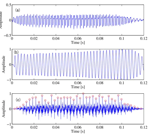
Figure 3.2: Example of GCI extraction on a voiced segment: (a) the speech signal, (b) its corresponding mean-based signal, (c) the LP residual with the detected GCIs.

Figure 3.2 (a) and (b) show a example of a voiced speech segment together with its corresponding mean-based signal. This latter presents the important property to evolve at the local pitch rhythm. However this signal in itself is not suﬃcient for accurately locating the GCIs. Indeed, the reported through our observations that a GCI occurs at a non-constant position between the minimum and the following positive zero-crossing of the mean-based signal.

The second step, we focus on LP residual signal. Intervals have been obtained and give short regions where particular events GCI should happen. The goal of the step is to associate an accurate location of an event within an interval. For this, we rely on the LP residual. Indeed, after removing an approximation of the vocal tract response, one can expect that signiﬁcant impulses in the excitation signal will be reﬂected in the LP residual. We can consequently assume that the event location corresponds to the strongest peak

(22)

of LP residual within the interval. Figure 3.2 (c) show the LP residual. Combining the intervals extracted from the mean-based signal with a peak picking on the LP residual allows toaccurately and unambiguously detect the GCIs. The GCIs position is loccted in red circle of LP residual signals as show in Figure 3.2 (c).

3.2.2 Estimation of GOI

Estimation of GOI is from Hilbert envelope (HE) of LP residual signal. Hilbert envelope is the magnitude of complex time function having signal and its Hilbert transformation as real and imaginary parts, respectively. The Hilbert envelope of a discrete time sequence s(n) is given by,

h[n] =|sa(n)| (3.2)

wheresa(n) is complex time function can be computed as follows,

sa(n) = s(n) + jsh(n) (3.3)

where sh(n) is Hilbert transform of s(n). The Hilbert transform is computed as

sh(n) = IDF T (SH(w)) (3.4) where SH(w) = { +jS(w) − π ≤ w < 0 −jS(w) 0≤ w ≤ π (3.5)

and S(w) is DFT of s(n). DFT refers to discrete Fourier transform and IDFT refers to inverse of DFT.

Therefore the magnitude of complex time function sa(n) is given by,

h(n) =

√

s2_{(n) + s}2

h(n) (3.6)

The GCI and GOI are not directly evident in the speech signal due to dominance of vocal tract information. For this, vocal tratc and excitation information needs to be separated. We use LP analysis and obtain LP residual, The LP residual mostly contains source information. The large error regoing during voiced speech can be attributed to GCI and GOI. The GCI in LP residual are characterized by the largest inpulse like discontinuities around GCI locations. However, the behaviour at the GOI is more regular since the excitation presents a discontinuity more spread out and with a weak strength. K. Ramesh found that the secondary peak in HE of LP residual is more prominent and less ambiguous than secondary peaks of impulse location in LP residual.

Figure 3.3 (a) plots the segment speech signal waveform, Figure 3.3 (b) is estimated GCI from the LP residual signals. The GCI estimated are used for estimating GOI from HE of LP residual. GOI are estimated by picking peaks between successive GCI locations in the HE of LP residual as shown in Figure 3.3 (c).

(23)

0 0.02 0.04 0.06 0.08 0.1 0.12 −0.5 0 0.5 (a) Time [s] Amplitude 0 0.02 0.04 0.06 0.08 0.1 0.12 −1 0 1 (b) Time [s] Amplitude 0 0.02 0.04 0.06 0.08 0.1 0.12 0 0.5 1 1.5 (c) Time [s] Amplitude

Figure 3.3: Example of GOI extraction on a voiced segment: (a) speech signal (b) LP residual with the detected GCIs are expressed by red circle , (c) HE of LP residual with the detected GOIs are expressed by green asterisk.

(24)

3.3 Analysis scheme

GCI and GOI are estimated as described in the previous section. The period (T0) is the

time duration between two consecutive GCIs. The scheme of analysis is shown in Fig. 3.4. We set some initial values for glottal sources value in one period, and waveform of LF model is constructed which can be used in the ARX process. The Kalman filter is used to estimate the time-varying coefficients of vocal tract filter. The re-synthesized speech waveform is estimated after the ARX process. The next step is to go to LF model again and a small random glottal source values instead of initial value in LF process, then go to ARX processed again. The optimal glottal source parameters is estimated by searching the smallest values of mean square equation error (MSEE) between original speech waveform and re-synthesized speech waveform.

Figure 3.4: Flowchart of ARX-LF model with accurate GCI and GOI

The detailed process is as follows:

• Estimation: get location of GCI and GOI in one period.

• Initialization: Te= (GCI-GOI)/T0, Tp=Te*0.65, Ta=(1-Te)*0.3, Ee=amplitude of

GCI. The waveform can be drew in this step.

• ARX model: implement Kalman ﬁlter. The re-synthesized speech will be repre-sented after this step.

• MSEE: calculate MSEE between original speech waveform and re-synthesized speech waveform.

(25)

• Loop: ARX model-MESS- LF model, search the smallest MSEE.

• LF model: Te+random number, Tp+random number, Ta+random number, Ee+random

number.

3.4 Database

Speech sentence is selected from the voice database of Fujitsu Lab. A vowel /a/ is selected from diﬀerent emotional speech state including neutral, joy, sad and anger. The sampling frequency is 12 KHz. The utterance is:

• I ra n/a/ i me-ru ga a ta ra su te te ku da sa i

3.5 Results and discussion

In this section, we give some analyzed results by our approach and compared with the approach of estimation of GCI parameter and GOI parameter in diﬀerent approach such as Motoda’s approach.

The results of four emotional states are plotted separately as follows. Each ﬁgure contains ﬁve panels; (a) is the waveform of LF model, in which we estimated the optimal

values of Tp, Te, Ta, and Ee. (b) is the vocal tract information, in which the peaks are

formant frequency. (c) is the LP spectrum envelope, in which we estimated the formant frequency by LP method. (d) is the error between the estimated signal and the orginal signal on our approach. (e) is the error between the estimated signal and the orginal signal of previous approach.

The results of neutral /a/ are plotted in Figure 3.5. The glottal source wave derivative (the waveform of LF model) is estimated in panels (a). The purpose of this research is foucs on glottal source imformation. However, since the ARX-LF model can eitimate the glottal source and vocal tract imforamation at the same time, that means if analyzed vocal tract imformation is correct, the glottal source also analyzed correct. Thus, the vocal tract imformation is extracted in panels (b). The peaks of (b) are formant frequency. In order to evaluate our approach, the LP spectrum envelope method to estimate the formant frequency is used, as shown in (c), in which the peaks are formant frequency. We can see that the formant frequency of LP spectrum envelope method similar with our results by compare (b) and (c), this point proves that our results is correct. The error between the estimated signal and the orginal signal is calculated, the error of our approach and the error of previous approach were plotted in (d) and (e). The results show that the error of our approach is smaller than previous approach.

The results of joy and anger speech are similar with the results of neutral speech as shown in Figure 3.6 and Figure 3.8. In case of sad speech, the results are show in Fig-ure 3.7. The estimated formant frequency of our approach is similar with the formant frequency of LP spectrum envelope method. The diﬀerent point is that the error of our

(26)

approach is similar with previous approach. The reason is that our approach used ARX-LF model with accrate GCI and GOI for analysis glottal source wave of emotional speech. The period of sad speech is much longer than neutral, joy and anger speech. Thus if GCI and GOI have small miatake, the results are aﬀected not so largely. So, the results of our approach is similar with the results of previous approach.

0.001 0.011 0.021 0.031 0.041 0.051 0.061 0.071 0.081 -0.20 0.2 _(a) Time(s) Amplitude 0.001 0.011 0.021 0.031 0.041 0.051 0.061 0.071 0.081 -0.20.2 (d)0 MSEE=0.0015 Time [s] Amplitude 0 1000 2000 3000 4000 5000 6000 -200 20 40 _(b) Frecuency[Hz] Amplitude [dB] 0 1000 2000 3000 4000 5000 6000 -200 20 40 Frequency [Hz] Amplitude [Db] (c) 0.001 0.011 0.021 0.031 0.041 0.051 0.061 0.071 0.081 -0.20 0.2 Time [s] Amplitude (e) MSEE=0.0068

Figure 3.5: Example of /a/ on neutral speech: (a) the waveform of LF model, (b) the vocal tract imformation, (c) the LP spectrum envelope, (d) the error of our result, (e) the error of previous result.

(27)

0.001 0.011 0.021 0.031 0.041 0.051 0.061 0.071 0.081 -0.50 0.5 (a) Time(s) Amplitude 0.001 0.011 0.021 0.031 0.041 0.051 0.061 0.071 0.081 -0.5 0 0.5 (d) MSEE=0.0055 Time [s] Amplitude 0 1000 2000 3000 4000 5000 6000 -200 20 40 _(b) Frecuency[Hz] Amplitude [dB] 0 1000 2000 3000 4000 5000 6000 -200 20 40 Frequency [Hz] Amplitude [Db] (c) 0.001 0.011 0.021 0.031 0.041 0.051 0.061 0.071 0.081 -0.50 0.5 Time [s] Amplitude (e) MSEE=0.0157

Figure 3.6: Example of /a/ on joy speech: (a) the waveform of LF model, (b) the vocal tract imformation, (c) the LP spectrum envelope, (d) the error of our result, (e) the error of previous result.

(28)

0.001 0.011 0.021 0.031 0.041 0.051 0.061 0.071 0.081 -0.10 0.1 (a) Time(s) Amplitude 0.001 0.011 0.021 0.031 0.041 0.051 0.061 0.071 0.081 -0.10 0.1 (d) MSEE=0.0005 Time [s] Amplitude 0 1000 2000 3000 4000 5000 6000 -200 20 40 _(b) Frecuency[Hz] Amplitude [dB] 0 1000 2000 3000 4000 5000 6000 -200 20 40 Frequency [Hz] Amplitude [Db] (c) 0.001 0.011 0.021 0.031 0.041 0.051 0.061 0.071 0.081 -0.10 0.1 Time [s] Amplitude (e) MSEE=0.0006

Figure 3.7: Example of /a/ on sad speech: (a) the waveform of LF model, (b) the vocal tract imformation, (c) the LP spectrum envelope, (d) the error of our result, (e) the error of previous result.

(29)

0.001 0.011 0.021 0.031 0.041 0.051 0.061 0.071 0.081 -0.50 0.5 (a) Time(s) Amplitude 0.001 0.011 0.021 0.031 0.041 0.051 0.061 0.071 0.081 -0.50 0.5 (d)_MSEE=0.0086 Time [s] Amplitude 0 1000 2000 3000 4000 5000 6000 -200 20 40 _(b) Frecuency[Hz] Amplitude [dB] 0 1000 2000 3000 4000 5000 6000 -200 20 40 Frequency [Hz] Amplitude [Db] (c) 0.001 0.011 0.021 0.031 0.041 0.051 0.061 0.071 0.081 -0.50 0.5 Time [s] Amplitude (e) MSEE=0.0227

Figure 3.8: Example of /a/ on anger speech: (a) the waveform of LF model, (b) the vocal tract imformation, (c) the LP spectrum envelope, (d) the error of our result, (e) the error of previous result.

(30)

3.6 Conclusion

The mean-based signal method for estimating GCI and the Hilbert envelope of LP residual method for estimating GOI can improve the accuracy of output of ARX-LF model. Thus, our apprpach is more suitable for estimating glottal source wave of emotional speech. The next section is to use our approach to analyze glottal source wave of emotional speech.

(31)

Chapter 4 Emotional speech analysis

The main purpose of this section is to analyze glottal source wave of emotional speech using our approach described in chapter 3.

4.1 Database

Emotional speech signals were selected from the voice database produced by Fujitsu lab-oratory. In this case, we selected six sentences from the database for analysis. The sentences are:

• A t/a/ ra shi i me-ru ga to do i te i ma su • Ma chi /a/ wa se ha a o ya ma ra shi i N de su • I ra n/a/ i me-ru ga a Q ta ra su te te ku da sa i • So N n/a/ no gu ru i me i shi N de su yo

• Te ga mi g/a/ to do i ta ha zu de su

• Ha n/a/ bi wo mi ru no ni go za ga i ri ma su ka

Each sentence contains four emotional states including neutral, joy, sad and anger,the phoneme /a/ is selected from the sentences for experiments.

(32)

4.2 Results

The mean values of parameters of the LF model in diﬀerent emotional speech are cal-culated. The mean values of parameters of the LF model are used for redrawing the waveform of the LF model in one period. Since the waveform of the LF model is glot-tal source wave derivative, the glotglot-tal source wave is the integral of waveform of the LF model. The glottal source waveform is calculated.

The results of six emotional speech are shown in the following ﬁgures. Each ﬁgure contains 8 panels: two panels in the top on the left are results of neutral speech which including waveform of the LF model and its integral, two panels in the top on the right are results of joy speech which including waveform of the LF model and its integral, two panels in the bottom on the left are results of sad speech which including waveform of the LF model and its integral, two panels in the bottom on the right are results of joy speech which including waveform of the LF model and its integral.

A example, glottal source spectral in the ﬁrst sentence is shown in Figure 4.2. The other glottal source spectral are similar with this example.

Finally, we also find out the relationship among different parameters of LF model in different emotional states. The results are as follows:

Tp: Anger < Joy < Neutral < Sad Te: Anger < Joy < Neutral < Sad

Ta: Anger ≈ Joy < Neutral < Sad

Ee: Anger ≈ Joy > Neutral > Sad

(33)

Table 4.1: Parameters of the LF model Tp Te Ta Ee T0 Neutral 1.51 ms 1.8 ms 0.135 ms 0.16 3 ms Joy 1.22 ms 1.47 ms 0.06 ms 0.27 2.3 ms Sad 3.57 ms 4.26 ms 0.22 ms 0.068 5.8 ms Anger 1.07 ms 1.25 ms 0.09 ms 0.26 2.5 ms 0 1 2 3 4 5 -0.2 0 0.2 Neutral Amplitude 0 1 2 3 4 5 0 0.05 time ms Amplitude 0 1 2 3 4 5 -0.2 0 0.2 Joy Amplitude 0 1 2 3 4 5 0 0.05 time ms Amplitude 0 1 2 3 4 5 -0.2 0 0.2 Sad Amplitude 0 1 2 3 4 5 0 0.05 time ms Amplitude 0 1 2 3 4 5 -0.2 0 0.2 Anger Amplitude 0 1 2 3 4 5 0 0.05 time ms Amplitude

Figure 4.1: /a/ of “a t/a/ ra shi i me-ru ga to do i te i ma su”, the glottal waveform derivative and glottal waveform in neutral, joy, sad and anger speech.

(34)

0 1000 2000 3000 4000 5000 6000 -40 -35 -30 -25 -20 -15 -10 -5 0 5 10 Frequency dB Neutral Joy Sad Anger

Figure 4.2: example: /a/ of “a t/a/ ra shi i me-ru ga to do i te i ma su”, glottal source spectral.

(35)

Table 4.2: Parameters of the LF model Tp Te Ta Ee T0 Neutral 1.6 ms 1.9 ms 0.11 ms 0.2 3.17 ms Joy 0.91 ms 1.26 ms 0.07 ms 0.23 2.33 ms Sad 4.52 ms 5.44 ms 0.35 ms 0.048 6.67 ms Anger 0.95 ms 1.14 ms 0.07 ms 0.27 2.25 ms 0 2 4 6 -0.2 0 0.2 Neutral Amplitude 0 2 4 6 0 0.05 time ms Amplitude 0 2 4 6 -0.2 0 0.2 Joy Amplitude 0 2 4 6 0 0.05 time ms Amplitude 0 2 4 6 -0.2 0 0.2 Sad Amplitude 0 2 4 6 0 0.05 time ms Amplitude 0 2 4 6 -0.2 0 0.2 Anger Amplitude 0 2 4 6 0 0.05 time ms Amplitude

Figure 4.3: /a/ of “ma chi /a/ wa se ha a o ya ma ra shi i N de su”, the glottal waveform derivative and glottal waveform in neutral, joy, sad and anger speech.the glottal waveform diﬀerentive and glottal waveform in neutral, joy, sad and anger speech.

(36)

Table 4.3: Parameters of the LF model Tp Te Ta Ee T0 Neutral 1.26 ms 1.5 ms 0.08 ms 0.15 3 ms Joy 1.17 ms 1.41 ms 0.04 ms 0.28 2.17 ms Sad 3.78 ms 4.56 ms 0.22 ms 0.05 6.17 ms Anger 0.89 ms 1.05 ms 0.06 ms 0.25 2.58 ms 0 2 4 6 -0.2 0 0.2 Neutral Amplitude 0 2 4 6 0 0.05 time ms Amplitude 0 2 4 6 -0.2 0 0.2 Joy Amplitude 0 2 4 6 0 0.05 time ms Amplitude 0 2 4 6 -0.2 0 0.2 Sad Amplitude 0 2 4 6 0 0.05 time ms Amplitude 0 2 4 6 -0.2 0 0.2 Anger Amplitude 0 2 4 6 0 0.05 time ms Amplitude

Figure 4.4: /a/ of “i ra n/a/ i me-ru ga a Q ta ra su te te ku da sa i”, the glottal waveform derivative and glottal waveform in neutral, joy, sad and anger speech

(37)

Table 4.4: Parameters of the LF model Tp Te Ta Ee T0 Neutral 1.32 ms 1.58 ms 0.08 ms 0.1 3 ms Joy 0.85 ms 1.03 ms 0.06 ms 0.22 2.08 ms Sad 4.66 ms 5.56 ms 0.23 ms 0.06 7 ms Anger 0.65 ms 0.79 ms 0.06 ms 0.3439 2 ms 0 2 4 6 -0.2 0 0.2 Neutral Amplitude 0 2 4 6 0 0.05 time ms Amplitude 0 2 4 6 -0.2 0 0.2 Joy Amplitude 0 2 4 6 0 0.05 time ms Amplitude 0 2 4 6 -0.2 0 0.2 Sad Amplitude 0 2 4 6 0 0.05 time ms Amplitude 0 2 4 6 -0.2 0 0.2 Anger Amplitude 0 2 4 6 0 0.05 time ms Amplitude

Figure 4.5: /a/ of “so N n/a/ no gu ru i me i shi N de su yo”, the glottal waveform derivative and glottal waveform in neutral, joy, sad and anger speech.

(38)

Table 4.5: Parameters of the LF model Tp Te Ta Ee T0 Neutral 1.64 ms 1.95 ms 0.05 ms 0.13 3.25 ms Joy 1.19 ms 1.4 ms 0.04 ms 0.21 2 ms Sad 4.53 ms 5.52 ms 0.16 ms 0.05 6.83 ms Anger 1.09 ms 1.32 ms 0.03 ms 0.22 2 ms 0 2 4 6 -0.2 0 0.2 Neutral Amplitude 0 2 4 6 0 0.02 0.04 time ms Amplitude 0 2 4 6 -0.2 0 0.2 Joy Amplitude 0 2 4 6 0 0.02 0.04 time ms Amplitude 0 2 4 6 -0.2 0 0.2 Sad Amplitude 0 2 4 6 0 0.02 0.04 time ms Amplitude 0 2 4 6 -0.2 0 0.2 Anger Amplitude 0 2 4 6 0 0.02 0.04 time ms Amplitude

Figure 4.6: /a/ of “Te ga mi g/a/ to do i ta ha zu de su”, the glottal waveform derivative and glottal waveform in neutral, joy, sad and anger speech.

(39)

Table 4.6: Parameters of the LF model Tp Te Ta Ee T0 Neutral 1.58 ms 1.87 ms 0.06 ms 0.14 3 ms Joy 0.81 ms 0.99 ms 0.06 ms 0.26 2 ms Sad 4.03 ms 4.94 ms 0.21 ms 0.05 6.25 ms Anger 0.76 ms 0.95 ms 0.02 ms 0.24 1.8 ms 0 2 4 6 -0.2 0 0.2 Neutral Amplitude 0 2 4 6 0 0.02 0.04 time ms Amplitude 0 2 4 6 -0.2 0 0.2 Joy Amplitude 0 2 4 6 0 0.02 0.04 time ms Amplitude 0 2 4 6 -0.2 0 0.2 Sad Amplitude 0 2 4 6 0 0.02 0.04 time ms Amplitude 0 2 4 6 -0.2 0 0.2 Anger Amplitude 0 2 4 6 0 0.02 0.04 time ms Amplitude

Figure 4.7: /a/ of “Ha n/a/ bi wo mi ru no ni go za ga i ri ma su ka”, the glottal waveform derivative and glottal waveform in neutral, joy, sad and anger speecp.

(40)

(41)

4.3 Discussion

For neutral speech, the result shows that the shape of glottal flow is similar to a sinusoidal wave. This is consistent with human speech production mechanism. When the airflow from lungs arrives at glottal fold, the glottal fold opens with a normal speed. Therefore, the glottal flow looks like a sinusoidal shape.

For joy speech and anger speech, the shape of glottal ﬂow looks like triangular wave. This result ﬁts with human speech production mechanism. As human is in the excited state when producing joy and anger speech, the position under glottis has high pressure, the glottal folds vibrate more quickly. Therefore, the shape is like triangular wave.

For sad speech the shape of glottal ﬂow is more smooth because air ﬂow arrives at glottal folds with a relatively slow speed which makes the glottal folds open slowly when human is in sad state.

A special parameter Ta is related to frequency energy. The smaller Ta is, the higher

frequency energy is. The results show that the high frequency energy of joy and anger speech is more than neutral speech, and much more than sad speech.

The results of Hiradate and Akagi [31] show that the power of anger speech is stronger than neutral speech, the stronger power is, the longer glottal closed time is in one period and the glottal source wave is more like trianguar wave. The results of this research also

show that the glottal closed time (T0-Te) of anger speech is longer than the glottal open

time and neutral speech. This results are consistent with the results [31]. However, we found that although the glottal source wave of joy speech look like trianguar shape, the glottal close time is not always longer than the glottal open time.

4.4 Conclusion

The glottal source wave of emotional speech was analyzed by using ARX-LF model with accurate GCI and GOI estimation approach. We obtained individual styles of glottal

source waves of diﬀerent emotional speech signals. These results are expected to be

further used for emotional speech conversion.

Figure 4.8 clearly show that the parameters of the LF model have big difference among neutral, sad and anger (joy). Thus, these results are very conducive for emotional speech conversion from neutral to sad speech, neutral to anger (joy) speech, sad to anger (joy) speech, and anger(joy) to sad speech. However, since the difference of parameters of the LF model is not so large between joy and anger speech, converting emotional speech from neutral to expected speech (joy and anger) is more difficult than others. These results show that the glottal source parameters have strong relationship with activation dimension. So the analyzed results can be used for converting different degree of emotional speech in activation dimension.

(42)

Chapter 5 Conclusion

5.1 Summary and contribution

In this thesis, the individual styles of glottal source waves of different emotional speech signals were obtained by ARX-LF model. The GCI and GOI were used as input parame-ters of LF model, in order to accurately estimate glottal source wave of emotional speech, the GCI and GOI were estimated by the mean-based signal method and the Hilbert enve-lope of LP residual method. The different parameters of LF model were obtained among different emotional speech.

The parameters of glottal source has strong relationship with activation dimension and can be used to convert diﬀerent degree of emotional speech in activation dimension.

5.2 Future work

The error of analyzed results of joy and anger speech is bigger than neutral and sad speech, thus more accurate approaches and parameters (such as GCI and GOI) should be considered to improve the results of analysis.

In this research, the time domain of LF model was considered, the frequency domain of LF model is also needed to be taken into consideration.

The vocal tract parameters should be considered for diﬀerent degree of emotional speech in valence dimension.

(43)

5.3 Acknowledgements

With the completion of this thesis, my master course at School of Information Science in JAIST will be close to the end. I would like to express my sincere gratitude to all those who have helped me for my study and life during the past two years.

My deepest gratitude goes ﬁrst and foremost to my supervisor, Professor Masato Akagi, he give me a lot of advise and help when i meet any problems both research and life.

Secondly, I would like to give my heartfelt gratitude to Associate Professor Masashi Unoki, Professor Jianwu Dang, Assistant Professor Daisuki Morikawa and Assistant Pro-fessor Ryota Miyauchi, for their invaluable comments and suggestions on my research.

(44)

Bibliography

[1] C. Veaux, X.robet, “Intonation conversion from neutral to expressive speech,” IN-TERSPEECH, pp. 2765-2768, 2011.

[2] Y. Stylianou, O. Cappe and E. Moilines, “Statistical methods for voice quality trans-formation,” Eurospeech, pp. 447-450, 1995.

[3] T. Toda, A. W. Black, K. tokuda, “ Voice conversion based on maximum-likelihood estimation of spectral parameter trajectory,” IEEE Trans. ASLP, Vol. 15, No.8, pp. 2222-2235, 2007.

[4] T. Toda, Y. Ohtani, K. Shikano, “One-to many and many-to-one voice conversion based on eigenvoices,” Acoustics, speech and signal processing, Vol. IV, pp. 1249-1252, 2007.

[5] T. Jianhua, K. Yongguo and L. Aijun, “Prosody conversion from neutral speech to emotional speech,” IEEE trans. Audio, speech and language processing. vol.14, pp. 1145-1153, 2006.

[6] A. Ryo, T. Ryoichi, T. Tetsuya and A. Yasuo, “GMM-based emotional voice conver-sion using spectrum and prosody features,” American journal of singal processing, pp. 134-138, 2012.

[7] H. Kawanami, Y. Iwami, T. Todo, H. Saruwatari and K. Shikano. “ GMM-based voice conversion applied to emotional speech synthesis” EUROPEECH, 208-211, 2003. [8] J. E. Cahn, “The generation of aﬀect in synthesized speech,” J. Amer. Voice I/O

Soc., vol. 8, pp. 1-19, 1990.

[9] C. Huang and M. Akagi. “A three-layered model for expressive speech perception. Speech communication, 810-828, 2008.

[10] H. Kawahara, et al, “Restructuring speech representations using a pitch-frequency-based F0 extraction: possible role of a repetitive structure in sounds,” Speech com-munication, Vol. 27, no. 3-4, pp. 187-207, 1999.

[11] S. Kristina and H. Barry, “Laryngeal motor cortex and control of speech in humans” Neuroscientist, 17(2), pp. 197-208, 2011.

(45)

[12] D. Klatt and L. Klatt, “ Analysis, synthesis, and perception of voice quality varations among female and male talkers,” J. Acoust. Soc. Am, vol. 87. pp. 820-857, 1990. [13] G. Fant, J. Liljencrants, and Q. Lin, “A four-parameter model model of glottal ﬂow,”

STL-QPSR4, pp. 1-13, 1986.

[14] G. Fant, “The LF-model revisited. transformation and frequency domain analysis,” STL-QPSR, 36 (2-3), 119-156, 1955.

[15] G. Fant, A. Kruckenberg, J. Liljencrants and M. Bavegard, “Voice source parameters in continuous speech. Transformation of LF-parameters,” Proc. ICSLP, Yokohama, pp. 1451-1454, 1994.

[16] P. Alku, “Glottal wave anlysis with potch synchronous lterative adaptive inverse ﬁltering,” Speech communication, vol. 11, pp. 109-118, 1992.

[17] O. Akande and J. Murphy, “ Estimation of the vocal tract transfer function with application to glottal wave anlysis,” Speech Communication, 46, 15-36, 2005.

[18] D. Weng, H. Kasuya and S. Adachi, “Simultaneous estimation of vocal tract and voice source parameters based on an ARX model,” IEICE Trans.Inf. Syst., Vol. E78-D, NO.6, pp. 738-743, June 1995.

[19] P. Michael D., Q. Thomas F. and R. Douglas A. “ Modeling of the glottal ﬂow derivative waveform with application to speaker identiﬁcation,” IEEE Transactions on speech and audio processing, Vol. 7, No.5, September 1999.

[20] D. Vincent, O. Rosec and T. Chonavel, “Estimation of LF model glottal source parameters based on arx model,” INTERSPEECH, pp. 333-336, 2005.

[21] Y. Agiomyrgiannakis, O. Rosec, “ ARX-LF-based source-ﬁlter methods for voice modiﬁcation and transformation,” ICASSP, 3589-3592, 2009.

[22] H. Motoda and M. Akagi, “A singing voice synthesis system to characterize vocal registers using ARX-LF model,” Proceedings of NCSP 2013, USA, pp. 93-96, 2013. [23] R. Elbarougy, M. Akagi, “ Speech emotion recognition system based on a dimensional

approach using a three-layered model,” APSIPA ASC, 2012.

[24] T. Chiba, and M. Kajiyama, “Its nature and struture,” Tokyo-kaiseikan Pub. Co, Ltd, 1941.

[25] J, Muller, “The physiology of the senses, voice, and muscular motion, with the mental faclties,” Pub. Taylor, Walton, London, 1848.

[26] G. fant, “Acoustic theory of speech production, (Mouton, the hague, netherlands),” pp. 15-90, 1960

(46)

[27] D. Vicent, O. Rosec and T. Chonavel, “A new method for speech synthesis and transformation based on an ARX-LF source-ﬁlter decomposition and hnm modeling” ICASSP, pp. 525-528, 2007.

[28] T. Drugman, T. Dutoit , “ Glottal closure and opening instant detection from speech signals,” in Proc. INTERSPEECH, 2009.

[29] T. Drugman, M. Thomas, J. Gudnason, P, Naylor and T. Dutoit, “ Detection of glottal Instants from speech signals: a quantitative review,” IEEE Transactions on audio, speech, and language processing, pp. 1-13, 2010.

[30] K. Ramesh, S. R. M. Prasana, D. Govind, “ Detection of glottal opening instants using Hilbert envelope,” INTERSPEECH, pp. 25-29, 2013.

[31] I. Hiradate and M. Akagi, “ Analyses of acoustic features of ”anger” emotional speech,” Technical report of IEICE. SP2001-141, 2002.

(47)

Publication list

Yongwei Li and Masato Akagi, “Analysis of emotional speech based on ARX-LF model for emotional speech conversion,” Proc. 2014 RISP International Workshop on Nonliner Circuits, Communications and Signal Processing, (to appear).

JAIST Repository: 感情音声変換のためのARX-LFモデルに基づいて感情音声の分析