Approximate Formulas for the Cell Loss Probability in Finite-Buffer Queues with Correlated Input

Approximate Formulas for the Cell Loss Probability in Finite-Buffer Queues with Correlated Input

Guidance

Professor Masao Fukushima Professor Tetsuya Takine

Shigeaki Maeda

2004 Graduate Course in

Department of Applied Mathematics and Physics Graduate School of Informatics

Kyoto University

KYOTO UNIVER SITY FO

U N^KYOTODED 1^JAPAN897

February 2006

Abstract

It is widely recognized that the Internet and video traffic indicate very bursty characteristics.

The queueing performance with this kind of traffic is likely to be different from that with the conventional Poisson traffic. From these points, analyzing and quantitatively evaluating the performance of queues with correlated input are of great importance. In particular, the loss probability in finite-buffer queues is the most important performance measure of interest.

In this thesis, we consider discrete-time single-server queues fed by correlated input and study the cell loss probability in finite-buffer queues. We study queues with two different types of input in detail. One is the long-range dependent (LRD) input, which has a subexponentially decaying autocorrelation function. The other is the generalized discrete-time autoregressive input, which is a generalization of the discrete-time autoregressive process of order one (DAR(1)) input and has a geometrically decaying autocorrelation function.

In the LRD input case, we propose an approximate formula for the cell loss probability in finite-buffer queues with LRD input. The approximate formula is constructed by studying an analytically tractable queueing model with LRD input, and it is asymptotically exact in this special case. Through numerical examples, the accuracy and robustness of the approximate formula are discussed throughly, and it is shown that the order of magnitude of the cell loss probability can be well estimated with the approximate formula.

In the generalized discrete-time autoregressive input case, we study queues fed by the gener-

alized discrete-time autoregressive input and construct an approximate formula for the cell loss

probability in finite-buffer queues with DAR(1) input, where we propose how to estimate the

asymptotic decay rate of the cell loss probability. Through numerical examples, the accuracy of

the approximate formula is examined, and it is confirmed that the formula works well when the

offered load is high or the correlation of the input is weak.

Contents

1 Introduction 1

2 Preliminaries 2

2.1 Discrete-Time Single-Server Queue . . . . 3

2.2 Autocorrelation Function of Correlated Input . . . . 3

3 Correlated Input Model and General Analysis 4 3.1 Mathematically Tractable Correlated Input Model . . . . 4

3.2 Analysis with Markov Chains . . . . 5

4 Queues with LRD Input 9 4.1 Approximate Formula for the Cell Loss Probability . . . . 9

4.2 Derivation of the Cell Loss Probability . . . . 10

4.2.1 LRD Input Model . . . . 10

4.2.2 Asymptotic Results . . . . 12

4.3 Numerical Results . . . . 14

4.3.1 Accuracy in Small Buffer Case . . . . 14

4.3.2 Accuracy and Robustness of Approximate Formula . . . . 16

4.3.2.A Queues with On/Off LRD Sources . . . . 17

4.3.2.B Queues with M/G/∞ Input . . . . 18

4.3.2.C Queues with Generalized Input . . . . 19

4.4 Conclusion . . . . 21

5 Queues with Generalized Discrete-Time Autoregressive Input 22 5.1 Generalized Discrete-Time Autoregressive Input . . . . 22

5.2 Asymptotic Analysis . . . . 22

5.3 Special Case: DAR(1) Input . . . . 24

5.3.1 Derivation of the Cell Loss Probability . . . . 24

5.3.2 Approximation of the Asymptotic Decay Rate . . . . 26

5.4 Numerical Results . . . . 30

5.5 Conclusion . . . . 33

6 Conclusion 33

Appendix A Proof of Lemma 1 i

Appendix B Proof of Lemma 3 i

Appendix C Proof of Lemma 4 ii

Appendix D Proof of Lemma 5 iii

Appendix E Proof of Lemma 6 iv

Appendix F Proof of Lemma 7 v

1 Introduction

It is widely recognized that the Internet traffic indicates very bursty characteristics so-called long- range dependence or self-similarity, e.g., see [21]. The queueing performance with this kind of traffic is likely to be different from that with the conventional Poisson traffic [15, 19]. Commonly used mathematical models for long-range dependent (LRD) and self-similar traffic are fractional Brownian motion, M/G/∞ input, and on/off source models with subexponential active periods [20], and many research papers have been published for the last decade [20, 22, 23]. Note here that most of those considered infinite-buffer queues and discussed the tail distributions of queue length and waiting time, e.g., [2, 22, 23]. In practice, however, the buffer size is finite and in these circumstances, the loss probability is the most important performance measure of interest.

Some efforts have been made to obtain the loss probability in finite-buffer queues with LRD input. Using the theory of large deviations, Likhanov and Mazumdar studied the asymptotic cell loss probability in a finite-buffer queue when the number of sources and the service rate go to infinity, while their ratio remains constant [13]. Tsybakov and Georganas obtain upper and lower bounds for the cell loss probability in a finite-buffer queue with M/G/∞ input [26]. The M/G/∞

input process is a vital traffic modeling tool because it is very flexible in time domain, i.e., the M/G/∞ input process can represent any autocorrelation function with respect to the numbers of arrivals if it is decreasing and convex [11]. However, the distribution of the number of arrivals in unit time is restricted to the family of Poisson distributions, and therefore the variation in space domain cannot be incorporated into the model. See also [10]. Zwart studies the asymptotic loss fraction in finite-buffer fluid queues when the buffer size goes to infinity [27]. See [14] also. To the best of our knowledge, however, there exists no handy formula to evaluate the loss probability in finite-buffer queues with LRD input.

This thesis develops a closed-form approximate formula for the cell loss probability in finite- buffer queues with LRD input. The past study on queues with LRD input and queues with heavy-tailed components show that the performance of those queues is determined mainly by the characteristics of LRD and heavy-tailed components, and other stochastic factors play a minor role. Thus we expect that the cell loss probability in queues with LRD input would be determined mainly by the correlation structure in the LRD input process. In other words, a loss probability formula in a specific queue with LRD input would be applicable to other queues, if the input processes of those queues have common characteristics.

Based on this observation, we study a discrete-time queue with a somewhat peculiar LRD input that is characterized by the distribution of the number of arrivals in unit time and two parameters related to the asymptotics of the autocorrelation function with respect to the number of arrivals. Even though this LRD input process is artificial, we can exactly analyze the stationary distribution of buffer contents, both in the finite-buffer and infinite-buffer queues. To the best of our knowledge, this LRD input model is the first one having such a feature. Further, we derive a closed-form asymptotic formula for the cell loss probability, combining the asymptotic tail distribution of buffer contents in the infinite-buffer queue [25] with the relationship between the stationary distributions of buffer contents in a finite-buffer queue and the corresponding infinite- buffer queue [9]. As you will see, the formula is given in terms of up to the second order statistics of the input process that can be readily computed. We then propose using this formula as an approximate formula for the cell loss probability in queues with LRD input.

The accuracy and robustness of the approximate formula are investigated by numerical exper-

iments. Because the approximate formula is derived based on the asymptotic cell loss probability

for large buffer, we first examine to what extent the approximate formula is accurate for relatively

small buffer systems, comparing with the exact result. Next we apply the approximate formula

to queues with LRD on/off sources, M/G/∞ input, and their generalized ones.

It is also interesting to consider the input that has a geometrically decaying autocorrelation function and a queue fed by this kind of input. For a few decades in the past, some input models with a geometrically decaying autocorrelation function were proposed and studied. One of the useful traffic models is the discrete-time autoregressive process of order one (DAR(1)).

The DAR(1) processes have been used as a model of video traffic [6] and queues with DAR(1) input were studied [7, 8]. The DAR(1) process has the following futures. In space domain, it can represent any distribution of the number of arrivals in unit time. On the other hand, in time domain, the autocorrelation function is determined by one parameter and it decays geometrically.

Hwang, Choi, and Kim studied the tail of the waiting time distribution with the theory of the GI/G/1 queue [7]. Hwang and Sohraby studied the queue length distribution and the mean queue length [8]. To the best of our knowledge, they considered and examined the infinite-buffer queues. In practice, however, the buffer size is finite, and in these circumstances, the cell loss probability is the most important measure.

In this thesis, we generalize the DAR(1) process and study finite buffer queues with this input.

In what follows, we call this input generalized discrete-time autoregressive input. Note here that the generalized discrete-time autoregressive input includes DAR(1) input as a special case and can represent any marginal distribution, which is similar to DAR(1). Further its autocorrelation function is given by discrete phase-type (PH) distribution whose number of parameters can be greater than one, while the number of parameters of DAR(1) is limited to only one. Thus, it is worth considering and studying the generalized discrete-time autoregressive input.

As in the case with LRD input, we consider finite buffer queues with generalized discrete-time autoregressive input and derive the cell loss probability using geometric asymptotics of Markov chains of M/G/1 type [25] with the relationship between the stationary distributions of buffer contents in a finite-buffer queue and the corresponding infinite-buffer queue [9]. Further, we consider the special case where the number of phases of discrete PH distribution of the input is equal to one, that is, DAR(1). We construct the approximate formula for the cell loss probability for DAR(1) input, where an approximate decay rate of the cell loss probability is proposed.

Through numerical examples, the accuracy of the formula is examined.

There are some common points in deriving approximate formulas for queues with LRD in- put and with the generalized discrete time autoregressive input. Thus we first derive the cell loss probability that is applicable to both cases. Next we study queues with LRD input and construct an approximate formula for the cell loss probability in finite-queues with LRD input.

We then consider queues fed by the generalized discrete-time autoregressive input and derive the approximate formula for queues with DAR(1) input.

The rest of this thesis is organized as follows. In section 2, we explain the discrete-time single-server queue and the input process. In section 3, we derive the cell loss probability in general settings. In section 4, we propose the approximate formula for the cell loss probability in queues with LRD input. In section 5, we study the cell loss probability with generalized discrete- time autoregressive input and construct the approximate formula for queues with DAR(1) input.

Finally, we conclude this thesis in section 6.

2 Preliminaries

In this section, we explain the discrete-time single-server queue and the terms and mathematical

definitions of the input process.

2.1 Discrete-Time Single-Server Queue

Throughout this thesis, we consider a stationary discrete-time single-server queue with a buffer of finite capacity N . We assume that the time axis is divided into slots with equal length. Let B

(n = 1, 2, . . .) and Q

(n = 0, 1, . . .) denote the numbers of cells arriving to the queue and present in the queue, respectively, at the nth slot. Given Q

, Q

is assumed to be determined by the following recursion: for n = 1, 2, . . .,

Q

= min

Q

− 1

+ B

, N

, (1)

where (x)

stands for max(x, 0). Let L

(n = 1, 2, . . .) denote the number of cells lost in the nth slot, i.e.,

L

=

Q

− 1

+ B

− N

, n = 1, 2, . . . .

We then define P

as the cell loss probability when the buffer size is equal to N : P

= lim

m→∞

P_m

n=1

L

Pm n=1

B

,

where the limit is assumed to exist with probability 1. In this thesis, we mainly study the cell loss probability P

.

2.2 Autocorrelation Function of Correlated Input

In this subsection, we introduce the important and useful indicators of input processes.

We define B as a generic random variable for B

’s. Further let γ(k) (k = 1, 2, . . .) denote the autocorrelation function of B

’s (n = 1, 2, . . .):

γ(k) = Cov[B

B

]

Var[B] , k = 0, 1, . . . .

It is well known that there exist two quite different types of correlation of the input. One is the input with the subexponentially decaying autocorrelation function and the other is the input with the geometrically decaying autocorrelation function.

We say that the autocorrelation function γ (k) of the input is subexponentially decaying if the input process {B

; n = 0, 1, . . .} satisfies

k→∞

lim γ(k)

k

= α,

where α > 0. In particular, if θ satisfies 0 < θ < 1, the input process is called LRD input [3]. We study queues with LRD input in section 4.

On the other hand, we say that the autocorrelation function γ(k) of the input is geometrically decaying, if the input process {B

; n = 0, 1, . . .} satisfies

k→∞

lim γ(k)

σ

= c

,

where 0 < σ < 1 and c

is some positive number. We call σ asymptotic decay rate. One example of this type of input is the generalized discrete-time autoregressive input. We study queues with this input process in section 5.

The autocorrelation function of the input represents a feature in time domain. On the other

hand, the marginal distribution of the input expresses a property in space domain. Generally

3 Correlated Input Model and General Analysis

In this section, we consider a discrete-time single server queue with a specific input process and derive the cell loss probability in finite buffer queues with this input. As we will see, we use the relationship between the stationary distributions of buffer contents in a finite-buffer queue and the corresponding infinite-buffer queue [9] and express the cell loss probability approximately in terms of the buffer contents in the corresponding infinite-buffer queue. Under the specific condition, the approximation becomes exact.

3.1 Mathematically Tractable Correlated Input Model

To explain our input model, the origin of time is set to be time −T + 1 (T > 0). The cell arrival process is then defined to be {B

; n = −T + 1, −T + 2, . . .}. We assume that there exists an underlying bivariate stochastic process {(Z

, D

); ν = 1, 2, . . .}, where Z

and D

take nonnegative and positive integer values, respectively, for all ν = 1, 2, . . .. Associated with this, the cell arrival process {B

; n = −T + 1, −T + 2, . . .} is determined in the following way. We define T

(ν = 1, 2, . . .) as

T

= −T +

n=1

D

, ν = 1, 2, . . . . (2)

B

(n = −T + 1, −T + 2, . . .) is then determined by

B

= B

= · · · = B

= Z

, ν = 1, 2, . . . ,

sample path wise, where T

= −T . Thus the cell arrival process is completely described in terms of the underlying bivariate stochastic process {(Z

, D

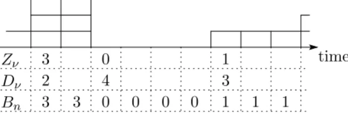
); ν = 1, 2, . . .}. Fig. 1 shows a sample path of the arrival process. For some ν, (Z

, D

) = (3, 2), so that three cells arrive in two consecutive slots. Next we have (Z

, D

) = (0, 4), and therefore no cells arrive in the next four consecutive slots. Further we have (Z

, D

) = (1, 3), so that one cell arrives in the next three consecutive slots, in this example.

3 2

3 3 0 1 1

4

1 0

0 0 0 1

Z

D

B

3

time

Fig. 1: Input model.

To make things tractable, we assume the followings.

Assumption 1

(i) Z

’s are independent and identically distributed (i.i.d.) random variables with finite mean and variance.

(ii) E[D

| Z

= m] = (1 − σ)

for all m = 0, 1, . . ., where 0 ≤ σ < 1.

(iii) Given Z

≥ 1, the conditional D

has the probability mass function d(l) (l = 1, 2, . . .), i.e., for all m = 1, 2, . . .,

Pr[D

= l | Z

= m] = d(l), l = 1, 2, . . . .

(iv) Given Z

= 0, the conditional D

follows a discrete phase-type (PH) distribution with irreducible representation (η, R), i.e.,

Pr[D

= l | Z

= 0] = ηR

r, l = 1, 2, . . . ,

where η and R denote a 1 × M probability vector and an M × M substochastic matrix, respectively, and r denotes an M × 1 vector which satisfies r = (I − R)e.

In what follows, we consider a situation such that T → ∞, and the input process {B

} is assumed to be stationary at slot 0. Let Z and B denote generic random variables for Z

’s and B

’s, respectively, in steady state. It then follows from Assumption 1 (ii) that Z and B have the same distribution. Thus we define b(m) (m = 0, 1, . . .) as

b(m) = Pr[Z = m] = Pr[B = m], m = 0, 1, . . . .

Note that Assumptions 1 (iii) and 1 (iv) are introduced so as to make the steady-state analysis simple.

3.2 Analysis with Markov Chains

In this subsection, we first consider a finite-buffer single-server queue with an input process satisfying Assumption 1. We then consider the relationship between the queue length distributions in the finite-buffer queue and in the corresponding infinite-buffer queue.

Recall that the queue length process {Q

; n = 0, 1, . . .} in the finite-buffer queue is governed by (1). Let ρ denote the expected number of cells arriving in a slot, i.e., ρ = E[B]. We define ρ

as the time-average probability of the server being busy. Since the service time of a cell is equal to the length of one slot, the cell loss probability P

is given by

P

= ρ − ρ

ρ . (3)

To obtain ρ

, we construct an embedded (bivariate) Markov chain, where all slots T

’s (see (2)) and all slots in which no arrival happens (B

= 0) are chosen as embedded Markov points.

Let X

(n = 1, 2, . . .) and H

(n = 1, 2, . . .) denote the number of cells in the system at the nth embedded Markov point and the length between the (n − 1)st and the nth embedded Markov points, respectively. Further we define G

(n = 1, 2, . . .) as the number of cells arriving in each slot during the nth interval H

. We then have

X

= min

(X

− 1)

+ A

, N

, n = 1, 2, . . . , where

A

= H

(G

− 1) + 1, n = 1, 2, . . . . (4) We introduce the phase variable S

(n = 1, 2, . . .) at the nth embedded Markov point:

S

=







0, if the nth embedded Markov point corresponds to T

for some ν, j, if the nth embedded Markov point does not correspond to T

for any ν

and the corresponding state of the discrete PH distribution of input is j.

It is readily seen that the bivariate process {(X

, S

); n = 1, 2, . . .} constitutes a Markov chain

Let A

(k = 0, 1, . . .) denote an (M +1)×(M +1) matrix whose (i+1, j+1)st (i, j = 0, 1, . . . , M ) element represents Pr[A

= k, S

= j | S

= i]. The transition probability matrix P

of the bivariate Markov chain {(X

, S

); n = 1, 2, . . .} is then given by

P

=













A

A

A

· · · A

A

A

A

A

· · · A

A

O A

A

· · · A

A

.. . .. . .. . . .. .. . .. . O O O · · · A

A

O O O · · · A

A













,

where A

=

A

. It is easy to see that the z-transform of A

’s (k = 0, 1, . . .) is given by A

(z) = A

(z) b(0)ηR

r R

!

, (5)

where

A

(z) = b(0)ηr +

X∞ l=1

b(m)d(l)z

.

Let X

and S denote generic random variables for X

’s and S

’s, respectively, in steady state. We then define x

(k = 0, 1, . . . , N ) as a 1×(M +1) vector whose (j+1)st (j = 0, 1, . . . , M ) element represents Pr[X

= k, S = j]. We denote (x

, x

, . . . , x

) by x

. Note that x

can be obtained numerically by solving x

= x

P

and x

e = 1, where e denotes a column vector with an appropriate dimension, whose elements are all equal to one. Some efficient numerical algorithms to solve those equations are available in the literature, e.g., see [12].

Let π denote a 1 × (M + 1) vector whose (j + 1)st (j = 0, 1, . . . , M ) element π

represents Pr[S = j]. Note that π satisfies πA

(1) = π and πe = 1. Thus we have







π

(1 − b(0) + b(0)ηR) + π

r = π

, π

b(0)ηR + π

R = π

,

π

+ π

e = 1,

where π

denote a 1 × M vector which means π

= (π

, π

, . . . , π

). Thus we obtain

π

= 1

1 + b(0)ηR(I − R)

e , π

= b(0)ηR(I − R)

1 + b(0)ηR(I − R)

e . (6) Let H denote a generic random variable for H

’s in steady state. We then have

E[H] = π

b(0) × 1 + (1 − b(0))E[D

]

+ (1 − π

) × 1

= b(0)η(I − R)(I − R)

e + (1 − b(0))η(I − R)

e + b(0)ηR(I − R)

e 1 + b(0)ηR(I − R)

e

= η(I − R)

e

1 + b(0)ηR(I − R)

e = π

E[D], (7)

where we use Assumptions 1 (ii) and 1 (iv) and (6).

Lemma 1 ρ

is given in terms of x

:

ρ

= 1 − x

e

E[H] . (8)

The proof of Lemma 1 is given in Appendix A. The following theorem is immediate from (3), (6), (7), and (8).

Theorem 1 Under Assumption 1, P

is given by P

= 1 − 1

ρ

1 − 1 − b(0) + b(0)E[D]

E[D] · x

e

.

Next we consider the corresponding infinite-buffer single-server queue with the same input process as in the finite-buffer queue. Let Q

(n = 0, 1, . . .) denote the number of cells at slot n in the corresponding infinite-buffer queue. We then have

Q

=

Q

− 1

+ B

, n = 1, 2, . . . .

We choose the same embedded Markov points as in the finite-buffer queue and construct the bivariate Markov chain {(X

, S

); n = 1, 2, . . .}, where X

denotes the number of cells in the system at the nth embedded Markov point. Note that X

’s satisfy

X

=

X

− 1

+ A

, n = 1, 2, . . . , where A

is given in (4).

It is clear that the transition probability matrix P

of the embedded bivariate Markov chain {(X

, S

); n = 1, 2, . . .} is given by

P

=













A

A

A

A

· · · A

A

A

A

· · · O A

A

A

· · · O O A

A

· · · O O O A

· · · .. . .. . .. . .. . . ..













.

To proceed further, we assume the following.

Assumption 2 E[B ] < 1.

Note that Assumption 2 ensures the existence of the steady state of the bivariate Markov chain {(X

, S

); n = 1, 2, . . .} [18]. We then define x

(k = 0, 1, . . .) as a 1 × (M + 1) vector whose (j + 1)st (j = 0, 1, . . . , M ) element represents Pr[X

= k, S = j], where X

denotes a generic random variable for X

’s in steady state. Because the transition probability matrix P

is of M/G/1 type, x

(k = 0, 1, . . .) can be obtained numerically by matrix-analytic methods [18].

We then use the following approximation of the stationary probability vectors of the bivariate Markov chain {(X

, S

); n = 1, 2, . . .} [9]:

x

≈ πA

e

k=0

x

A

e · x

. (9)

Remark 1 Note here that A

is given by A

= b(0)

1

!

·

1 − σ σ

,

when M = 1. Thus we can utilize the relationship between the stationary distributions of buffer contents in the finite-buffer queue and the corresponding infinite-buffer queue in [9]. Namely, using Lemmas 1 and 2 in [9], we obtain

x

= πA

e

k=0

x

A

e

· x

, i.e., the approximation given in (9) becomes exact.

Theorem 2 Under Assumptions 1 and 2, P

is given in terms of x

’s:

P

≈ 1 − ρ

ρ · x

A

e

πA

e − x

A

e , (10) where

x

=

x

.

When M = 1, the approximation given in (10) becomes exact, i.e., P

= 1 − ρ

ρ · x

A

e

πA

e − x

A

e . (11)

Proof: In the same way as in the proof of Lemma 1, we have ρ = 1 − x

e

E[H] . (12)

It then follows from (8), (9), and (12) that

ρ

= 1 − (1 − ρ) x

e x

e

≈ 1 − (1 − ρ) πA

e

k=0

x

A

e . (13)

Substituting (13) into (3) yields

P

≈ 1 − ρ ρ

πA

e

k=0

x

A

e

− 1

!

. Thus noting π =

x

, we obtain (10).

From Remark 1, the approximation in (13) becomes exact when M = 1. Thus we obtain (11) when M = 1.

The results obtained in this section are used in section 4 and 5 to derive the approximate

formulas for the cell loss probability.

4 Queues with LRD Input

In this section, we consider the cell loss probability in finite buffer queues with LRD input.

4.1 Approximate Formula for the Cell Loss Probability

This subsection presents an approximate formula for the cell loss probability. We now present an approximate formula for P

, assuming {B

; n = 1, 2, . . .} is a stationary sequence of random variables. We define B as a generic random variable for B

’s. Further let γ(k) (k = 1, 2, . . .) denote the autocorrelation function of B

’s (n = 1, 2, . . .):

γ(k) = Cov[B

B

]

Var[B] , k = 0, 1, . . . .

Proposition 1 Suppose 0 < E[B ] < 1, 0 < Var[B] < ∞, and there exist α (α > 0) and θ (0 < θ < 1) such that

k→∞

lim γ(k)

k

= α. (14)

P

is then approximately given by

P

≈ c(θ)γ(N ), (15)

with

c(θ) = B(θ)

E[B]

"

1 − Pr[B = 0]

C

[B]

#

,

where C

[B] = Var[B ]/E[B]

denotes the squared coefficient of variation of B and B(θ) =

X∞ m=2

(m − 1)

Pr[B = m].

Because 0 < θ < 1, (14) implies that the input process {B

; n = 1, 2, . . .} is LRD [3]. The approximate formula in (15) is asymptotically exact for a certain queueing model considered in the next subsection. We observe the followings from this formula:

(i) The cell loss probability P

is (asymptotically) proportional to the autocorrelation func- tion γ(N ), i.e., lim

P

/γ(N ) = c(θ), where c(θ) is given in terms of E[B ], C

[B], Pr[B = 0], and B (θ).

(ii) When Var[B] is finite, the characteristics of the tail distribution Pr[B > k] has no impact on the cell loss probability. Note that, in telecommunication networks, B is bounded above by channel capacity, so that the assumption of finite variance does not matter at all in application.

(iii) The factor B(θ) can be obtained numerically, whereas it may be hard to obtain explicit

expressions for mathematical models.

(iv) Because B(θ) (0 < θ < 1) is an increasing function of θ, the upper and lower bounds of the asymptotic constant c(θ) are readily obtained to be

c(0) < c(θ) < c(1), where

c(0) = E[B ] − (1 − Pr[B = 0]) E[B]

"

1 − Pr[B = 0]

C

[B]

#

,

c(1) = Var[B] + (1 − E[B])

− Pr[B = 0]

E[B ]

"

1 − Pr[B = 0]

C

[B]

#

.

(v) Based on the observation in (iv), we obtain a conservative approximate formula for P

:

P

≈ c(1)γ(N ), (16)

whose accuracy may be estimated in advance if the ratio c(1)/c(0) is known.

The advantage of the conservative approximate formula (16) is obvious; it provides an explicit formula for a specific mathematical model. For example, consider a single-server queue with M/G/∞ input [11]. In this case, B follows a Poisson distribution with mean ρ, and therefore we have

P

≈ ρ + (1 − ρ)

− exp(−ρ)

ρ(1 − ρ exp(−ρ)) · γ (N ), (17)

if 0 < ρ < 1 and (14) holds. Note that the ratio c(1)/c(0) in M/G/∞ input is an increasing function of ρ and lies in (1, e − 1) for 0 < ρ < 1. Therefore we expect that (17) can be used to estimate the order of magnitude of the cell loss probability in single-server queues with M/G/∞

input. For more details, see subsection 4.3.

4.2 Derivation of the Cell Loss Probability

In this subsection, we consider a discrete-time single-server queue with a specific LRD input process, which is given by introducing some assumptions to the model described in section 3, and derive the asymptotic cell loss probability given on the right hand side of (15).

4.2.1 LRD Input Model

We consider input process considered in section 3 again. In addition to Assumption 1, we assume the following.

Assumption 3 M = 1, i.e., η = 1, R = σ, r = 1 − σ, and

Pr[D

= l | Z

= 0] = (1 − σ)σ

, l = 1, 2, . . . .

In what follows, we use the following notation for simplicity in description.

f (k) ∼

g(k) ⇐⇒ lim

k→∞

f(k) g(k) = 1.

Let D

denote a generic random variable for the conditional D

given Z

≥ 1.

Assumption 4 There exist θ (0 < θ < 1) and β (0 < β < ∞) such that Pr[D

> k] ∼

βk

.

Remark 2 Note that for real x ≥ 0

Pr[D

> x] = Pr[D

> bxc]

bxc

∼ β(bxc)

, where bxc denotes the integer part of x. Because

x

≤ (bxc)

≤ (x − 1)

= x

1 − 1 x

_−(θ+1)

, we obtain

x→∞

lim

Pr

D

> x

βx

= 1, from which it follows that

x→∞

lim

Pr[D

> tx]

Pr[D

> x] = t

.

Thus Assumption 4 implies that Pr[D

> x] is regularly varying at ∞ with index −(θ + 1) [1].

Theorem 3 Under Assumptions 1, 3, and 4, the autocorrelation function γ(k) of the B

satisfies

γ (k) ∼

αk

, (18)

where

α = β

θE[D] 1 − b(0) C

[B]

!

. (19)

Remark 3 Because 0 < θ < 1, Theorem 3 implies that the stationary input process {B

; n = 0, 1, . . .} is LRD under Assumptions 1, 3, and 4.

Proof: We define B

(n = 1, 2, . . .) as the number of cells arriving in slot n given that T

= 0 for some ν . Let D

denote a random variable representing the forward recurrence time of D

, i.e.,

Pr[ D

= n] = Pr[D

> n]

E[D

] , n = 0, 1, . . . .

We then have for k = 1, 2, . . ., E[B

B

] − E[B ]

=

k−1X

j=0

X∞ m=1

m Pr[B = m, D

= j]E[B

] +

m

Pr[B = m, D

≥ k] − E[B ]

= E[B]

k−1X

j=0

Pr[ D

= j]E[B

] + Var[B] Pr[ D

≥ k] − E[B]

Pr( D

< k)

= Var[B] Pr[ D

≥ k] − E[B]

k−1X

j=0

(E[B] − E[B

]) Pr[ D

= j].

Thus we obtain

γ(k) = Pr[ D

≥ k] − 1

C

[B] · g(k), (20)

where

g(k) = 1 E[B]

k−1X

j=0

(E[B] − E[B

]) Pr[ D

= j]. (21) Lemma 2 (Bingham et al. [1]) Under Assumption 4, we have (see the proof of Corollary 8.10.4 in [1])

Pr[ D

≥ k] ∼

1

θE[D] · βk

. (22)

Lemma 3 Under Assumptions 1, 3, and 4, we have g(k) ∼

b(0)

θE[D] · βk

. (23)

The proof of Lemma 3 is given in Appendix B. (18) now follows from (20), (22), and (23).

4.2.2 Asymptotic Results

In this subsection, we derive the asymptotic cell loss probability when N → ∞ under Assumption 4 (i.e., assuming the LRD input process).

Theorem 4 Under Assumptions 1, 2, 3, and 4, x

satisfies x

∼ π

B (θ)βN

θ(1 − ρ)E[H] · π. (24)

Proof: (5) implies that [A

]

= 0 for all k = 1, 2, . . . unless i = j = 0. Also for k ≥ 1,

A

0,0

=

[A

]

= Pr[H

(G

− 1) + 1 ≥ k + 1, S

= 0 | S

= 0]

= Pr[H

(G

− 1) > k − 1 | G

≥ 1, S

= 0, S

= 0]

· Pr[G

≥ 1, S

= 1 | S

= 1]

= Pr[D

(Z − 1) > k − 1 | Z ≥ 1] Pr[Z ≥ 1]

=

b(m) Pr

D

> k − 1 m − 1

. (25)

Lemma 4 Under Assumption 4,

m=2

b(m) Pr

D

> k − 1 m − 1

k

∼ B(θ)β(k − 1)

, (26)

holds.

The proof of Lemma 4 is given in Appendix C.

Using (25) and (26), we obtain

A

0,0

∼

B(θ)βk

, and therefore we have

A

∼

k

C, where

C = B(θ)β 0

0 0

!

.

Thus our model satisfies Assumption 4 in [25]. Using Remark 12 in [25], we obtain x

∼ πCe

x

e

k

· π.

Further, noting (12) and

πCe = π

B(θ)β, we have

x

∼

π

B (θ)β (1 − ρ)E[H]

X∞ k=N

k

· π. (27)

Because

∞ N

x

dx <

X∞ k=N

k

<

Z _∞

N

(x − 1)

dx, we obtain

X∞ k=N

k

∼

N

θ . (28)

Applying (28) to (27) yields (24).

Theorem 5 Under Assumptions 1, 2, 3 and 4, P

satisfies P

∼

B(θ)

E[B]

"

1 − b(0) C

[B]

#

· αN

, (29)

where α is given in (19).

Proof: Note that (11) holds when M = 1. Applying (24) to (11), we obtain

P

∼ 1 − ρ ρ ·

π

B (θ)βN

θ(1 − ρ)E[H] · πA

e πA

e − π

B(θ)βN

θ(1 − ρ)E[H] · πA

e

= 1 − E[B]

E[B] · π

B (θ)βN

θ(1 − E[B ])E[H] − π

B(θ)βN

N

∼ π

B (θ)βN

θE[B]E[H] , (30)

where we use ρ = E[B ]. Substituting (7) into (30), we obtain P

∼

B(θ)

E[B] · β

θE[D] · N

. (31)

(29) now follows from (19) and (31).

4.3 Numerical Results

The approximate formula (15) stems from the asymptotic cell loss probability for large buffer.

Thus it is not clear to what extent parameters in LRD traffic affect the accuracy of the formula in the small buffer case, even for the model studied in subsection 4.2.1. Thus we first discuss this aspect. Next we investigate the accuracy and robustness of the approximate formula by comparing it with simulation results for queues fed by a superposition of independent on/off LRD sources, M/G/∞ input process, and their generalized ones.

4.3.1 Accuracy in Small Buffer Case

This subsection discusses the accuracy of the approximate formula (15) when the buffer size is small. To do so, we compare the approximate results with those obtained by exact analysis in subsection 3.2. For a while, we assume that the number of cells arriving in a slot in steady state follows a geometric distribution, i.e.,

b(m) = 1 1 + ρ

ρ 1 + ρ

m

, m = 0, 1, . . . . (32)

Further we assume that

Pr[D

≥ l] = 1

l

, l = 1, 2, . . . .

10⁻³ 10⁻² 10⁻¹ 1

10¹ 10² 10³ 10⁴

P_loss^(N)

Buffer SizeN ρ=.4, exact ρ=.4, eq.(15) ρ=.8, exact ρ=.8, eq.(15)

Fig. 2: Exact and asymptotic cell loss probabilities (θ = .5).

10⁻⁴ 10⁻³ 10⁻² 10⁻¹ 1

10¹ 10² 10³ 10⁴

P_loss^(N)

Buffer SizeN θ=.2, exact

θ=.2, eq.(15) θ=.5, exact θ=.5, eq.(15) θ=.8, exact θ=.8, eq.(15)

Fig. 3: Exact and asymptotic cell loss probabilities (ρ = .6).

Fig. 2 shows the exact and approximate (i.e., asymptotic) cell loss probabilities as a function of the buffer size, where θ = .5. We observe that the approximation is accurate even for a queue with small buffer when the load is light. In a heavily loaded situation, however, the approximate formula slightly underestimates the cell loss probability in queues with small buffer.

Next we examine the impact of θ on the accuracy of the approximation. For this purpose, we set ρ = .6. Fig. 3 shows the exact and approximate cell loss probabilities as a function of the buffer size. We observe that the difference between the exact and approximate results becomes small with θ. Thus we expect that the approximate formula is accurate when correlation in arrivals is strong.

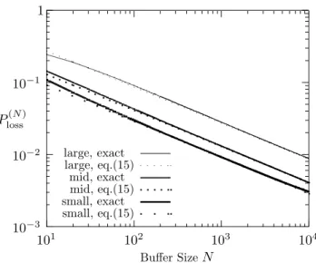
Finally, we examine the impact of the variance of B on the accuracy of the approximation.

For this purpose, we set ρ = .6 and θ = .5. As a distribution with modest variance, we choose a

geometric distribution given in (32). Note that E[B ] = .6, Var[B] = 0.96, and b(0) = 5/8 in this

case. Besides, we prepare two multi-point distributions, which are given by the solutions of the

10⁻³ 10⁻² 10⁻¹ 1

10¹ 10² 10³ 10⁴

P_loss^(N)

Buffer SizeN large, exact

large, eq.(15) mid, exact mid, eq.(15) small, exact small, eq.(15)

Fig. 4: Exact and asymptotic cell loss probabilities (ρ = .6, θ = .5).

following linear programming problems:

(P-small) minimize

k

b

subject to b

≥ 0 (k = 1, 2, . . . , 10),

k=1

b

= 1 − b(0),

X10 k=1

kb

= ρ.

(P-large) maximize

k

b

subject to b

≥ 0 (k = 1, 2, . . . , 10),

k=1

b

= 1 − b(0),

X10 k=1

kb

= ρ.

As a result, for a distribution with small variance, we have 3-point distribution with b(1) = 2(1 − b(0)) − ρ = 3/20 and b(2) = ρ − (1 − b(0)) = 9/40 (Var[B] = .69), and for a distribution with large variance, we have 3-point distribution with b(1) = [10(1 − b(0)) − ρ]/9 = 7/20 and b(10) = [ρ − (1 − b(0))]/9 = 1/40 (Var[B ] = 2.49). Fig. 4 shows the exact and approximate cell loss probabilities as a function of the buffer size. We observe that the approximation is accurate when the variance of B is large.

In summary, the approximate formula is fairly accurate even in the small buffer case, and at worst it seems to be used to estimate the order of magnitude of the cell loss probability. Besides, the approximate formula (15) is likely to underestimate the cell loss probability, and therefore the conservative approximate formula (16) might be more suitable for an engineering purpose. This will be discussed further in the following subsection.

4.3.2 Accuracy and Robustness of Approximate Formula

In this subsection, we apply the approximate formula to queues fed by a superposition of inde-

pendent on/off LRD sources and M/G/∞ input, and compare the approximation with simulation

results. Generally speaking, it is rather hard to conduct simulation experiments for rare events in

stochastic models with LRD and/or heavy-tailed components. To overcome this difficulties, we adopt a pseudo-random number generator called the Mersenne Twister [16], which has a period of 2

− 1 and 623-dimensional equidistribution property

. The Mersenne Twister enables us to generate very long sample paths.

4.3.2.A Queues with On/Off LRD Sources

We consider a finite-buffer queue with K independent and homogeneous on/off sources. Each source becomes on and off alternately, and on- and off-periods form a discrete-time alternating renewal process. While being on, each source generates exactly one cell in each slot, and no cells are generated in off-periods.

We define F

and F

as generic random variables for the lengths of on- and off-periods, respectively. Let µ

= E[F

] and µ

= E[F

]. We assume that F

has a discrete Pareto distribution with shape parameter θ + 1, i.e.,

Pr[F

> l] =

1

l + 1

, l = 0, 1, . . . ,

where 0 < θ < 1. Note that µ

=

(1/l)

. Let ρ denote the overall traffic intensity. We then have ρ = Kµ

/(µ

+ µ

), from which it follows that µ

= (K − ρ)µ

/ρ. We assume that F

has a geometric distribution, i.e.,

Pr[F

> l] =

1 − 1 µ

_l

, l = 0, 1, . . . .

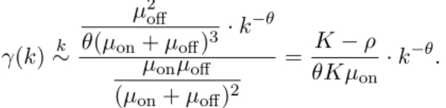
Because sources are homogeneous, the correlation coefficient γ(k) (k = 1, 2, . . .) of the numbers of cells arriving at lag k is identical with that of an individual source. Further, because the variance of the number of cells generated by a source is given by µ

µ

/(µ

+ µ

)

, it follows from Theorem 4.3 in [5] that

γ(k) ∼

µ

θ(µ

+ µ

)

· k

µ

µ

(µ

+ µ

)

= K − ρ θKµ

· k

.

On the other hand, the number B of cells arriving in a slot follows a binomial distribution, i.e., for m = 0, 1, . . . , K,

Pr[B = m] = K m

!

ρ K

m

1 − ρ

K

.

We conduct regenerative simulation experiments for queues with on/off sources described above. Because off-periods of each source are geometrically distributed, time instants n such that (X

, B

) = (0, 0) are regenerative points. We then define a regenerative cycle as an interval between regenerative points, during which at least one cell arrives (i.e., an idle period and the fol- lowing busy period). All simulation results given below are obtained from 10 billion regenerative cycles. Further 95% confidence intervals are shown. Note that in computing the 95% confident intervals, we regard 1,000 successive regenerative cycles as a unit cycle, due to lack of memory capacity.

Fig. 5 shows the cell loss probability P

for ρ = .4 and .8 as a function of the buffer size N , where K = 5 and θ = .5. We observe that when ρ is small, the approximate formula (15) bounds

1A pseudo-random number generated by the Mersenne Twister is composed of a 53-bit fixed point part and a

10⁻³ 10⁻² 10⁻¹

10¹ 10² 10³ 10⁴

P_loss^(N)

Buffer SizeN ρ=.4

ρ=.8

simulation eq.(15) eq.(16)

Fig. 5: Queues with on/off LRD sources (K = 5, θ = .5).

10⁻⁴ 10⁻³ 10⁻² 10⁻¹ 1

10¹ 10² 10³ 10⁴

P_loss^(N)

Buffer SizeN θ=.2

θ=.5

θ=.8 simulation

eq.(15) eq.(16)

Fig. 6: Queues with on/off LRD sources (K = 5, ρ = .6).

P

from the above, whereas it slightly underestimates P

when ρ is large. On the other hand, the conservative formula (16) works well in both cases. Fig. 6 shows P

for θ = .2, .5 and .8 as a function of the buffer size N , where K = 5 and ρ = .6. We observe that when θ is large (i.e., correlation is weak), the approximate formula (15) provides an upper bound of P

. However, it slightly underestimates P

when θ is small. The conservative formula (16) works well in all cases.

4.3.2.B Queues with M/G/∞Input

Next we consider queues with M/G/∞ input. Note that the M/G/∞ input process is obtained

as the limit K → ∞ in the model described above, while ρ remains constant and the distribution

of F

is fixed. Thus the number B of cells arriving in a slot follows a Poisson distribution with

mean ρ, and the correlation coefficient γ(k) (k = 1, 2, . . .) of the numbers of cells arriving at lag

10⁻³ 10⁻² 10⁻¹

10¹ 10² 10³ 10⁴

P_loss^(N)

Buffer SizeN ρ=.4

ρ=.8

simulation eq.(15) eq.(17)

Fig. 7: Queues with M/G/∞ input (θ = .5).

10⁻⁴ 10⁻³ 10⁻² 10⁻¹ 1

10¹ 10² 10³ 10⁴

P_loss^(N)

Buffer SizeN θ=.2

θ=.5

θ=.8

simulation eq.(15) eq.(17)

Fig. 8: Queues with M/G/∞ input (ρ = .6).

k is given by [11]

γ(k) = 1 µ

X∞ l=k

1 l

θ+1

∼

1 θµ

· k

. (33)

We conduct simulation experiments in exactly the same way as in the case of queues with on/off LRD sources. Fig. 7 shows the cell loss probability P

for ρ = .4 and .8 as a function of the buffer size N , where θ = .5. Also, Fig. 8 shows P

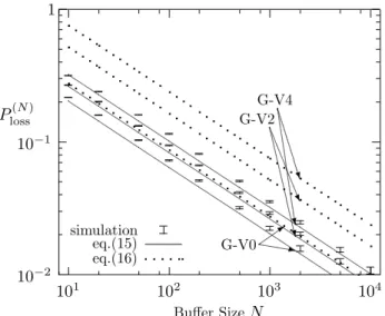
for θ = .2, .5 and .8 as a function of the buffer size N , where ρ = .6. Form these two figures, we observe that the general tendency of the accuracy of approximation for M/G/∞ input is very similar to that for a superposition of on/off LRD sources given in Figs. 5 and 6. It is worth noting that such a simple formula (17) works very well.

4.3.2.C Queues with Generalized Input

In queues with on/off LRD sources (resp. M/G/∞ input), the distribution of B is restricted to

a family of binomial (resp. Poisson) distributions. Thus we discuss the accuracy and robustness