Article
Financial Crisis of Finland, Sweden, Norway and Japan*
Shigeyoshi Miyagawa Yoji Morita
Department of Economics Kyoto Gakuen University
Kyoto, Japan
Correspondence (Fax): +81 771-292388
Abstract
The aim of the paper is to research the financial crisis occurred in Nordic countries and Japan in the early 1990s. The Nordic countries’ experiences of bubble, bust, and financial crisis are compared with Japan’s experience.
These countries had suffered from the mounting nonperforming loans after the bust of the bubble. The Nordic countries successfully achieved renewed economic growth, while the Japanese recession had been prolonged. The first part of the paper will analyze the mechanism and the background behind the emergence and bust of the bubble in Nordic countries and Japan.
In the second part of the paper, on the full awareness of the chorological explain of the development of the crisis, the Vector Error Correction Model will be applied into Finland and Japan. The model will examine whether or not there exists a long-run equilibrium relationship between the money stock and economic activity, paying attention to the precautionary money demand caused by the financial anxiety. People are expected to increase the precautionary demand, facing the financial crisis. The survey data will be used to quantify the financial anxieties in both countries. The estimation results suggest that the cointegration property still hold in both countries.
Keywords: bubble, financial liberalization, money stock, cointegration, financial anxieties
JEL classification: E21, E22, E24, E44
* Original version of the paper was presented at the seminar held at the School of Business and Economics, University
of Jyväskylä, Finland, on August 28, 2009. The author wishes to thank Professor Kari Heimonen, Professor Jaakko
Pehkonen and other staff for their useful comments and suggestions.
1. Introduction
The U.S. subprime mortgage problem has triggered the turmoil in the global financial markets since the fall of 2008. The Japanese economy which gradually recovered form the long recession after the bust of the bubble in 1990 has also been severely damaged. The Nikkei Stock average has fallen down to the level of 7000 yen, a critical level, under which the Japanese financial system will almost collapse. The bubble and the bust of the bubble historically repeated themselves since the Great Depression in 1930s. The paper focuses on the bubble and the bust of the bubble happened in the period around 1990. The aim is to analyze the cause of the bubble and clear the mechanism behind the emergence and expansion of the bubble, comparing Japan’s experiences with those of Nordic countries.
Nordic countries realized the advanced welfare states with full employment policy and strong labor union policies. Their successful economic and social policies suddenly collapsed when they had the mounting nonperforming loans (NPLs) after the rapid increase of asset prices in the latter half of 1980s. Japanese economy also has the same experience, though the economic and social system is different. Japanese economy was on the verge of financial panic, especially in 1997 and 1998, when major financial institutions had failed.
The Nordic countries successfully achieved renewed economic growth, while the Japanese recession had been prolonged. What are the common background factors behind the radical fluctuation of the asset prices?
The paper will be divided into two parts. In section 2, the paper will chronologically review the economies before and after the bust of the bubble in Finland, Sweden, Norway and Japan. The financial distress and deflation is rooted in the bubble economy of the latter half of the 1980s when the economy had experienced the financial deregulation. The review in Section 2 will clear how the economic bubble occurred, how the recession started with the collapse of the bubble and how the authority, government and central bank responded to its deterioration.
In section 3, on the full awareness of the chorological explain of the development of the crisis, the Vector Error Correction Model will be applied. Finland and Japan will be picked up because the statistical data of both countries are well equipped and easily accessible. The model will examine whether or not there exists a long-run equilibrium relationship between the money stock and economic activity, paying attention to the precautionary money demand caused by the financial anxiety. The financial panics increase the financial anxieties among the people. People are expected to increase the precautionary money demand, facing the financial crisis. The rapid rise in the money demand might break out the long-run equilibrium relationship between the money stock and the economic activity. The survey data will be used to quantify the financial anxieties in both countries. The estimation results suggest that the cointegration property among money stock and economic activities still hold in both countries.
2. The financial crisis in Nordic countries
In Nordic countries, credit rapidly expanded in the around 1985 because of the financial
deregulation. Three countries, Finland, Sweden, and Norway had experienced the rapid rise
and fall in the asset price in the years around 1990. In Denmark, the asset inflation was not so sharp as in other three countries
1. Banks became very competitive to make a loan to the commercial and residential property as well as stock. Because of the strong competition, nominal interest rates were kept at a low level. Moreover real interest rates were even lower, sometimes negative due to the inflation and tax advantage. Expanded loan rapidly increased the asset prices. The rise in asset prices enhanced the capability of firms and households to borrow funds. Asset prices rapidly increased and created the speculative bubbles. However its bubble was suddenly busted. The bust of bubble caused an amount of NPLs which hampered the financial system. The collapse of the banking system damaged the real sector of the economy through the disintermediation of the credit. The process of the rapid rise and fall of the asset prices in Finland, Sweden, Norway and Japan will be examined in the next section.
2-1 Finland
2The Finnish economy had experienced a severe recession in 1990s. Real GDP rapidly decreased from 1990 to 1993. The GDP growth rate fell more than 14 percent for 4 years. It reached at a peak in 1990, and then declined sharply toward the end of 1992 as reported in Figure 1. The depression was caused by the financial liberalization at first. As a consequence of the financial liberalization, bank lending rapidly expanded especially after 1985 and peaked in 1990 as shown in Figure 2. Capital inflow from foreign countries also contributed to the increase of lending booms.
Financial liberalization itself does not cause the rapid asset price inflation. When the financial markets are deregulated under the monetary easing, the asset price increases.
Money stock started to increase gradually. Year on year growth rate of Money stock (M1) reached at a peak, 17.7 percent in 1989q1. M2 growth rate also peaked at 18.4 percent in 1988q1. Both growth rates sharply declined after its peak as shown in Figure 3.
A strong similarity among the countries experienced the financial crisis is observed regarding the timing of financial liberalization and asset inflation. In Finland the indirect finance was dominant while the direct finance was not developed well before the 1980s when the financial deregulation started. Deposits banks were centre to the financial market.
Deposit banks also controlled the firms through financing. In Finland the periods of the bubble and its bust are as follows. The bubble period is from 1985 to 1990 while the depression by the bust of bubble is from 1991 to 1993.The average GDP growth rate from 19985 to 1990 was 3.4 percent. The bubble has started around 1986.The factors behind the bubble can be summarized in the following three factors.
First factor is the financial liberalization. The security market rapidly developed and
1 The reasons why the asset inflation was not strong in Denmark come from the fact that the country had joined the European Economic Community (now the European Union). As a result, the deregulation process had already started around 1975 and interest rates were relatively high to meet the exchange rate targets within the European Monetary System. See Howells Peter and Keith Bain (2008) P. 175.
2 This section mainly depends on Kalela, Kiaander, Kivikuru, Loikkanen & Simpura, (2002), Nyberg and
Vihriala(1994), Honkapohja, Seppo, Erkki Koskela, Willi Leibfritz, and Roope Uusitalo (2009).
10.00 10.04 10.08 10.12 10.16 10.20 10.24
85 86 87 88 89 90 91 92 93 94 95 LNRGDP
(Source) OECD database
Figure 1 log (real GDP)
24000 28000 32000 36000 40000 44000 48000 52000 56000 60000
85 86 87 88 89 90 91 92 93 94 95 Non-bank private, Public. government/Includes MFIs/mill (Source) OECD database
Figure 2 Bank lending
-.10 -.05 .00 .05 .10 .15 .20
85 86 87 88 89 90 91 92 93 94 95
DM1 DM2
(Source) OECD database
Figure 3 Money Stock (growth rate)
borrowing from abroad substantially increased because of the abolition of exchange rate control in the latter half of 1980s. The liberalization of bank lending rate and private borrowing from abroad brought about the rapid expansion of bank loan and large capital inflow from foreign countries. Second is the sharp improvement of the terms of trade. The decline of oil price and the rise in world market prices of forest products promoted the Finnish export. Third is the monetary easing. Average money growth rate is more than 10%
in 1986-87 as reported in Figure 3.
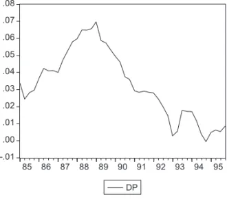
The inflation rate gradually began to increase in the boom. Consumer prices rose from around 2 % in 1986 to around 8% in 1990 reported in Figure 4. The rapid rise in inflation rate weekend the Finnish export competitiveness and caused serious current account problems. Under the deregulation and monetary easing, banks became very competitive to find the borrowers. Especially savings banks became very aggressive to risk taking. Banks’
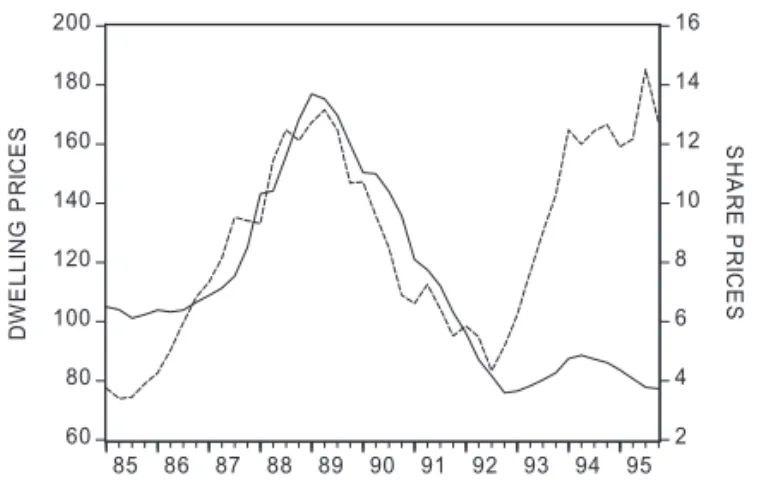
profits gradually declined with the progress of financial liberalization in Finland too, as reported in Table 1. In addition, capital inflow from foreign countries rapidly increased. As a consequence, the real estate and other assets price substantially increased as shown in Figure 5.
The economic boom had turned around in 1990 when the real GDP started to decline.
The GDP continued to decline by the fall of 1993. The Finnish exports gradually decreased with a decline of the price competitiveness and the deterioration of terms of trade. Moreover, the collapse of Soviet Union strongly reduced the Finnish exports to Russia. Finnish exports to and imports from Russia quickly dropped by 70% in 1991
3. The economic loss by a negative demand shock of the collapse of Soviet Union including indirect effects is estimated about 2.5% of GDP
4. The rise of interest rate in Europe after German unification
-.01 .00 .01 .02 .03 .04 .05 .06 .07 .08
85 86 87 88 89 90 91 92 93 94 95 DP
(Source) OECD database
Figure 4 Consumer Price Change
3 Honkapohja, Seppo, Erkki Koskela, Willi Leibfritz, and Roope Uusitalo (2009) P. 17.
4 See Nyberg and Vihriala (1994).
also contributed to the decline of the Finnish economy, through the tight monetary policy.
Unfortunately for Finland, a speculative attack on the Markka had begun from 1990.
Bank of Finland had to take a tight monetary policy to protect their currency. However, a tight monetary policy had seriously damaged the Finnish economy.
With the fall in the economy, asset prices started to decline and bankruptcies of firms began to increase. By mid-1991 the number of bankruptcies had increased to a monthly average of some 600 from around a year before
5. The NPLs which banks hold rapidly accumulated in 1991-92. Some 40 % of banks’ NPLs were related to construction, real estate and retail trade
6. The financial crisis had occurred. The banks which were most severely damaged were the savings banks. They had aggressively expanded the loans during the boom. They increased the loans to small firms and property related firms. Unfortunately, many of their loans were denominated in foreign currencies. So the depreciation of the Markka strongly damaged their borrowers. As a consequence Skopbank, a central bank of the saving banks was the first commercial bank which became insolvent. The banking problems continued and were the worst in 1992.
The Finnish Markka was devaluated in November 1991 and changed to the floating system in September, 1992. Bank of Finland was relieved of its legal obligation to keep the exchange rate at the decided zone. As well known as the irreconcilable trinity of an open economy in international finance, three objectives; fixed exchange rate system, independent monetary policy and free international capital flows, cannot be achieved simultaneously.
Under the new currency regime Bank of Finland came to implement freely monetary policy concentrating on the domestic economy. Bank of Finland also decided to take inflation target with the change of exchange rate regime. Price level targeting framework is a signal that
60 80 100 120 140 160 180 200
2 4 6 8 10 12 14 16
85 86 87 88 89 90 91 92 93 94 95 DWELLING PRICES / HELSINKI / Real price index(1983Y=100) / FIM SHARE PRICES/ALL SHARES/ INDEX PUBLICATION BASE/2000Y=100
DWELLINGPRICES SHAREPRICES
(Source) OECD database
Figure 5 Asset Prices
5 See Chart 13 in Nyberg and Vihriala (1994).
6 The banks’ NPLs rapidly increased from FIM 42 billion to FIM 77 billion during 1992. See Nyberg and Vihriala
(1994).
BOF would not cause inflation. This framework contributed to mitigate concerns that new exchange rate system might eventually lead to the inflationary economy. The government injected public funds to the problem banks in the form of preferred capital certificates in early 1992. Government Guarantee Fund (GGF) was set up in order to support the banking system. Public injection continued through 1994. The public funds totally injected to the financial system reached at 7.5% of the 1992 GDP
7. The depreciated Marrka also contributed to the rise in exports. As a result, the Finnish economy rapidly recovered since 1994.
2-2 Sweden
8In Sweden the financial deregulation has started in the early 1980s. The liquidation ratio for banks was abolished in 1983. Interest ceilings were lifted in the spring of 1985. The lending ceilings for banks and the placement requirements for insurance companies were abolished in 1985. The financial intermediaries rapidly expanded the credits as a result of the financial deregulation. Banks, mortgage institutions, and finance companies freely compete to make a loan. The total loan expanded by 136 % from 1986 to 1990. Money stock rapidly increased as shown in Figure 6. A housing boom arose and housing prices sharply increased. Growth rate of housing prices are shown in Figure 7. A tax advantage also contributed to the rise of the housing boom. When people borrow from banks to buy house, interest payments were fully deductible from taxable income. High-leverage financial investments were used in the stock market. The stock market became active and stock prices continued to rise. It reached at a peak in August 1989. The unemployment rate continued to decline and reached at a record low level in 1989. Both high inflation expectation and a tax advantage reduced the after-tax real inertest rate to a very low level.
-.08 -.04 .00 .04 .08 .12
1985 1986 1987 1988 1989 1990 1991 1992 MM
Figure 6 Money Growth Rate in Sweden
7 The corresponding figures for Sweden and Norway are 5.2 and 3 percent, respectively. See S. Honkapohja and others (2009) p. 24.
8 The section mainly depends on Peter Englund (1999) and Timothy Edmonds (2008).
However the bubble suddenly busted after 1990, when monetary policy was tightened.
A tax reform also contributed to the sharp decline of asset prices. A deduction of the interest payments from taxable income was severely constrained by the reform. Both the tightening of monetary policy and tax reform busted the bubble in Sweden. After there were reports of difficulties in finding tenants at current levels in the autumn of 1989, real estate market began to decline
9. The stock market also negatively reacted and started to decline. Especially real estate stock price index had declined by 52 per cent from its peak level
10. The growth rate of both prices of commercial and dwelling buildings is reported in Figure 7. The bust of the bubble was triggered by a tight monetary policy. The radical change of monetary policy was caused by international interest rate hike following the German reunification and Riksbank’s policy change to focus on inflation. The tax reformed also negatively affected the asset markets
11. The financial crisis has started in Sweden when one of the finance companies Nyckeln could not roll over maturing marknadsbevis in September 1990. Other finance companies also bankrupted due to the rapid shrink of marknadsbevis markets. The financial crisis spread to the whole financial system because the commercial banks lend funds to the finance companies. Two of the six major banks, Första Sparbanken and Nordbanken caused solvency problems.
The response of the Swedish government was very prompt. They strongly supported the financial system, announcing they will guarantee all deposits of banks. The public funds were swiftly injected to save the problem banks.
The currency market was unstable in the summer of 1992, especially after Finland started the floating system on September 8, 1992. The Riksbank was obliged to increase the
-20 -10 0 10 20 30
82 84 86 88 90 92 94 96 98 00 02 04 06 08 COMMERCIAL BUILDING DWELLING BUILDING
Figure 7 Growth Rate of Housing Prices
9 Peter Englund (1999), P.89.
10 Peter Englund (1999), P.89.
11 The marginal tax on capital income and interest deductions was reduced from 50% for most taxpayers to a flat 30 %
as part of a major tax reform becoming effective in 1991. P. Englund (1999), P.89.
overnight call rate to 500 % to protect the krona. Sweden decided to move to the floating system at last. The Riksbank began to take an easy monetary policy under the new exchange rate regime. Money stock rapidly increased. Both the government funds injection and a new exchange rate system contributed to the early recovery of the Swedish economy.
2-3 Norway
12The Norway’s financial crisis was not so severe as those in Finland and Sweden. The crisis occurred a few years before those in Finland and Sweden. Asset price inflation did not continue so long due to the oil price fall in 1986. A speculative attack against krone was not so fierce as in Finland and Sweden, because krone was not so overvalued before the attacks began in the early 1990s
13. However it is true that the financial crisis strongly damaged the Norwegian economy.
In Norway, banks were heavily regulated in both the quantity and rates for their lending by the mid-1980s as in other Nordic countries. The interest rates were artificially kept at a low level. The excess demand for lending was controlled by the credit rationing. Banks were also required to invest in government bonds. Foreign exchange and international capital movements were also strongly regulated. The government controlled the financial system through the subsidized loans to politically important sectors, such as the residential sector, and industrially depressed regions in the northern Norway. They still continued to provide the subsidized funds on a large scale even after the housing are already enough.
The strongly regulated financial system was kept even after government changed to a conservative party. The reasons why Norway preferred to keep a government controlled financial system are summarized in the following three factors
14. 1. Strong political pressure groups gained considerably from the subsidized loans. 2. Norwegian politicians had strong anti-market sentiments. 3. Many households and firms had lots of debts. High debts of the firms and households have been special features of the Norway’s credit market. However the Central Bank and Ministry of Finance was obliged to follow the international trend toward deregulation
In 1984 a financial deregulation has started in Norway, which has triggered the excessive credit expansion. Due to the abolition of the regulation of new branch establishments, the number of branches rapidly increased. The branches of commercial banks and savings banks increased by 15% and 5.5% respectively from 1983 to 1987. The number of employees had increased by 28% in savings banks and by 19% in commercial banks from 1983 to 1987. The loans mainly expanded to the newly established small firms, real estate, construction, and services industries. The lending by financial institutions to firms and households grew at 12% from 1984 to 1986, roughly three times the average growth rate in the years prior to deregulation
15.
12 The section mainly depend on E. Steigum (1992) and Timothy Edmon eds. (2008).
13 When Norges Bank let the krone float, it fell by only 4 per cent. Later it recovered. This initial fall was much smaller than the depreciation registered in Finland and Sweden. See Lars Jonung and others (2009).
14 E. Steigum (1992), P.3.
15 E. Steigum (1992), P.11.
The easy monetary policy continued until Norges Bank (Central Bank of Norway) raised interest rates to protect the Kroner from depreciating in December 1986. The commercial banks expanded the loans under the fierce competition with non-bank financial institutions which were less regulated under the easy monetary conditions. The bank credits had rapidly increased in the period 1984-1987. The money stock also rapidly increased during 1986 as reported in Figure 8. The real after-tax interest rate became almost zero.
Thus, not only firms but also households increase the borrowing from financial institutes to buy house, cottage, and yachts and even expensive holidays abroad
16. As a consequence, assets prices rapidly increased. The price of housing had increased by 40% in the period 1984 -1987. The share prices also rapidly increased by 1987 as reported in Figure 9. The expanded loan contributed to the rise of asset prices, which enhanced the value of borrowers’
assets as their collateral, which in turn promoted bank lending.
0 4 8 12 16 20
1985 1986 1987 1988 1989 1990 1991 MM2
Figure 8 Money Growth Rate (M2) in Norway
10 12 14 16 18 20 22 24
1985 1986 1987 1988 1989
SHARE PRICES/ALL SHARES SHARE PRICES/INDUSTRIES
Figure 9 Share Price (Norway)
16 E. Steigum (1992), P.9.
The oil price had rapidly declined in 1986 as shown in figure 10. Petroleum-related industries which are main industries in Norway were damaged. However the restrictive fiscal policy was implemented in 1987 and 1988 to reduce the real disposable income of households and to reduce imports. Monetary policy was also tightened to defend the fixed exchange rate system in December 1986. The recession had started in 1988 when both housing prices and the share price started to decline. The real estate prices fall down by 40%
from mid-1987 to 1991. The deepest recession continued from 1988 to 89. Bankruptcies rapidly increased from 1426 in 1986 to 3891 in 1988 and 4536 in 1989
17. In 1987, the leading bank, Den Norsuke Creditbank suffered a huge loss. In 1989 a medium sized bank, Norion Bank was bankrupted. NPLs kept to accumulate. The banking crises had got worse in 1991. The government decided to inject public funds to the banks in 1991 and 1992.
The Central Bank underestimated the effect of the financial deregulation on credit supply and aggregate demand. They targeted nominal interest rate in their monetary policy.
The politician did not agree to take a tight monetary policy. The largest political party, the Labor Party had insisted a lower nominal interest rate in its 1985 election campaign, though after tax real interest rate was very low. The nominal interest rate targeting policy seems to make the Central Bank to keep the easy policy. When the oil price started to decline in 1985
18, the Central Bank began to supply lots of liquidity into the banks in order to avoid the rise of nominal interest rate, which fueled the expansion of credit. The supply of such liquidity loans increased to 80 billion kroner in 1986
19. This easy monetary policy prolonged the credit expansion and the boom in Norway.
10 15 20 25 30 35 40
1976 1978 1980 1982 1984 1986 1988 1990 1992 Oil Price
Figure 10 Oil Price (Norway), us$/barrel
17 E. Steigum (1992), P.14.
18 During 1986, the price of North Sea Brent Blend crude oil fell from $27 a barrel to $14.50 a barrel. T. Edmonds (2008) P.11.
19 E. Steigum (1992), P.12.
2-4 Japan
As in the Nordic countries, an important factor in the Japanese financial crisis is the financial liberalization that started in the 1980s. The Japanese bubble had also appeared with the progress of financial liberalization under easy money condition. As it was in the Nordic countries, Japanese financial system was highly regulated by the government. The interest rate was artificially kept at a low level in order to reduce the fund raising cost of the main industries. The household have to endure the lower interest rate than the rate they could earn on the deposit. It was a kind of subsidy transferred from the household to the industries.
The Ministry of Finance strictly controlled the banks with the strong power. Security market was also strongly regulated. A cooperate finance mainly depended on the indirect financing through the financial intermediaries. The direct finance was less developed as in the case of Nordic countries.
The financial liberalization had started in the security markets. With the removable of the restriction on the fund-raising in the securities market, the major firms became less dependent on the banks. On the contrary, the liberalization of interest rates on the deposits was gradual. As a consequence the profits of the banks gradually declined. They are obliged to seek new lending opportunity among small business and property-related firms. See Table 1 which shows that financial liberalization reduced the banks’ profits.
However financial liberalization itself does not cause the asset inflation. The most important factor behind the asset price inflation is the monetary easing. The monetary easing compounded with the liberalization caused the rapid asset inflation. The reason why monetary easing occurred in Japan can be explained as follows. Mounting Japanese trade surplus was often condemned by other countries, especially by United States of America.
The trade friction between Japan and U.S got worse year by year, especially after President Ronald Reagan started so-called Reaganomics by adopting monetarist policy and supply side policy. His policy, targeting a low inflation rate and strong dollar, had caused twin deficit of trade and budget in U.S. The U.S trade deficit with Japan accounted for over half of its total trade deficit in the 1980s. U.S congress took very hard stance to the Japanese increasing trade surplus and threatened with retaliating trade measures.
U.S. demanded to open the meeting to discuss the U.S huge trade deficit. The Minister of Finance and governor of the central bank of G5 countries (United States, United
Table 1 Interest Margins of Commercial Banks (net interest income/assets)
1980 1984 1987 1990 1991
Finland 2.28 1.65 1.57 1.60 1.25
Sweden 2.26 2.21 2.49 2.08 2.09
Norway 3.50 3.30 2.78 2.63 2.49
Japan 1.61 1.36 1.20 0.90 1.11
(Sources) Shigemi (1995)
Table 1 Interest Margins of Commercial Banks (net interest income/assets)
1980 1984 1987 1990 1991
Finland 2.28 1.65 1.57 1.60 1.25
Sweden 2.26 2.21 2.49 2.08 2.09
Norway 3.50 3.30 2.78 2.63 2.49
Japan 1.61 1.36 1.20 0.90 1.11
(Sources) Shigemi (1995)
Kingdom, France, West Germany, and Japan) gathered to Plaza Hotel in New York in 1985.
They discussed how to correct the trade imbalance between U.S and Japan and West Germany, especially how to reduce the huge trade deficit in U.S.
G5 countries had agreed to concert to depreciate the high dollar in the meeting. The cooperative interest reduction had begun. In 1985, a long-term interest rate in U.S was 10.8 percent, while that in Japan was 5.8 percent. The difference was 4.7 percent as shown in Figure 11, when the exchange rate was 250s yen per dollar. In August 1986, US’s interest rate was reduced to 7.3 percent while Japan’s rate was 5.2 percent. The difference was reduced to 2.1 percent, which caused the rapid yen’s depreciation from 250s to 150s.
However Japanese current account balance did not decrease in spite of the yen’s appreciation. US government was afraid that the further appreciation of the yen would make the Japanese economy so stagnant and would be counter productive to the U.S economy.
Japanese economy was in the slight recession due to the high yen after Plaza agreement.
Thus, U.S gave the pressure to stimulate the Japan’s domestic demand and to raise the imports.
In the February 1987 Louvre agreement, Japan was required to take much easier monetary policy. The Bank of Japan reduced the official discount rate to 2.5 percent, then the lowest level (Figure 11). Money growth started to rise in 1987 Q1. It grew more than 10 percent from 1987 Q1 through 1990 Q2 (Figure 12). It was the beginning of the Japanese bubble.
Under the assumption of affluent funds available, banks were very aggressive and competitive in their loan business. Anybody could get loans very easily from the banks as far as they had lands as the collateral because land price was believed to keep increasing forever. Large firms could get funds easily by using “equity finances”. So banks had tried to
(source) Bank of Japan
Figure 11 Official Discount Rate: US and Japan
expand the loans to small firms and property-related firms. Both the stock and land prices had rapidly increased from 1988 through 1989, which could not be explained rationally by the fundamentals.
Japanese bubble was busted as follows. The BOJ implemented the third rise of discount rate from 3.75 to 4.25 percent in December 1989 when a new BOJ governor Yasuo Mieno had taken his office. However the market was still bullish. Land and stock prices continued to rise to levels that could not be rationalized by the fundamentals of the Japanese economy.
He had showed very strong stance to the bullish economy by the fourth rise of discount rate from 4.25 to 5.25 percent. Mieno was hailed as an “Onihei of Heisei era”, a famous police leader, who had strongly fought against the gangs in the Edo era more than 200 years ago.
The bubble was mainly discussed from the view point of income and asset distribution. This Mieno’s episode reflect well the public feeling that “bubble-busting” was a right minded from ethical view point.
He took the role of arbitrage of asset prices, unfortunately for the Japanese economy
20. Furthermore governor Mieno had implemented the fifth rise of discount rate to 6.0 percent to avoid the homemade inflation caused by the Gulf War in August 1990 as shown in Figure 11. In addition the government also placed a ceiling on the total amount of financing available for real estate purchase.
The bust of the bubble began at last. The money stock (M2+CD) rapidly declined. It recorded negative year on year growth in mid –1992 as shown in Figure 12. After hitting a record high of 38,915 yen at the end of 1989, the stock price (Nikkei Dow-Jones Index) rapidly began to decline. In August 1992, stock price dipped below 15,000 yen, a 63 percent plunge from a peak level in Figure 13. Land price began to fail after hitting a peak in September 1990 and kept falling until now as shown in Figure 14. In response to the asset
(source) Bank of Japan
Figure 12 Money Growth Rate (year on year)
20 Nowadays many economists understand that central bank should not take the role of the arbitrage of asset prices.
See Randal Parker (2002).
price decline, the BOJ reduced the discount rate six times from July 1991 to February 1993.
The discount rate was ultimately reduced from 6.0 percent to 2.5 percent in Figure 11. The government also implemented the fiscal stimulus by spending a total of 29.9 trillion yen in two years from 1992 to 1993.
Land and stock prices were promoted to decline. Prices continued to decline and increased the deflationary pressure. Firms were obliged to continue the adjustment of their balance sheet damaged by the decline of asset prices. The banks were left holding a big amount of NPLs. It was jusen which had first got the severest damage by the NPLseven Jusen were set up by the Japanese major bank, which decided to get into the mortgage lending market in the bubble period. When all seven jusen became insolvent after the bust of the bubble, the NPLs was estimated over 6 trillion yen at the time.
(source) Tokyo Stock Exchange
Figure 13 Stock Price (Nikkei Dow-Jones Index )
(source) Japan Real Estate Institute, 6 Large Urban Areas, average (residential, commercial, and industrial)
Figure 14 Change of Land Price (year on year)
The Japanese economy began to show the signs of a modest recovery in late 1995, when real GDP began to increase and the official estimation of NPLs decreased. The Ministry of Finance had issued a report entitled “Reorganizing the Japanese Financial system (kinyu shisutemu no kinoukaifuku nituite)” in June 1995, in which they showed a diehard attitude to tackle the NPLs problems by officially disclosing the magnitude of bad loans totalled 40 trillion yen (about 4 percent of the loans held by depository institutions).
Furthermore the MOF strongly pledged the complete deposit guarantee by March 2001, with a reform of the Deposit Insurance Corporation and Prompt Corrective Act, which had been already implemented with a success in the United States in 1991 after the financial crisis in the end of 1980s. As a result the financial anxieties had been dispelled in 1995.
However Prime Minister Hashimoto, worried about the future of the government finance, implemented measures to reconstruct the financial structure. He was afraid that fiscal condition would get worse and worse with the coming of aging society in Japan. He decided to increase the consumption tax from 3 to 5 percent and abolish a special income tax cut in April 1997, which amounted to a tax increase of 9 trillion yen. Consumption had rapidly shrunk in response to Hashimoto’s tax increase policy. Unfortunately for the Japanese economy, the East Asian economic crises occurred in July 1997. The fiscal contraction compounded by the Asian crisis decreased the aggregate demand substantially.
Under the deflationary conditions, a financial panic occurred. Hokkaido Takushoku Bank, one of Japan’s city banks (largest twenty banks), and Yamaichi Securities Company, one of Japan’s four largest security companies, failed in November 1997
21. The failure of
(source) Bank of Japan
Figure 15 Price Change (GDP deflator)
21 The first bank failure since the Second World War is Tokyo-based Cosmo Credit Corporation, Japan’s fifth-largest
credit union, in July 1995.
two big financial institutions sent the sign that the government gave up the “too big to fail”
policy. People thought no financial institutions were immune from failures. Rumors about the other banks’ failure had spread out through Japan. The stock prices of many financial institutions sharply declined and “Japan premium” in the international money market jumped by around 100 basis points. Japanese banks were obliged to pay the additional basis points for raising funds in the oversea financial markets. The premium is calculated as the difference between the quoted rates of TIBOR in the Tokyo offshore market and LIBOR in the London offshore market. Bonds issued not only by Japanese financial institutions but also by Japanese government were downgraded at the investment grade ratings by international credit-rating agencies, such as Moody’s.
In response to the serious situation, the government decided to provide 30 trillion yen funds by issuing bonds. The government was not willing to inject public funds into the problem banks by considering the negative sentiments of the congress and public at first.
However the financial panic was so severe that neither the congress nor the public strongly opposed an injection of public funds to assist the problem banks. The 30 trillion yen was divided into the following two categories: 13 trillion yen was prepared for the enforcement of the Deposit Insurance System, while the remaining 17 trillion yen was intended for the capital injection of the problem financial institutions.
The government actually injected 1.8 trillion yen to 21 large banks to raise their capital ratio in March 1998. However it had no significant effect on the banks because it was lax.
Long-Term Credit Bank and Nippon Credit Bank had failed in 1998 after the injection of public funds. 7.5 trillion yen was again injected in March 1999. The implementation was quite different from the former injection. Banks were strongly required to submit a detailed and meaningful restructuring plan
22.
The government hesitated to quickly resolve the NPLs and bank problems which weakened financial institutions and prolonged the recession. The government officially announced in late 1995 that NPLs totaled 38 trillion yen, 4 percent of outstanding loans. In 1998, NPLs increased to 73.1 trillion yen, 12 percent of all loans or 10 percent of GDP. All efforts by the government and private banks to decrease NPLs did not succeed in reducing them at all because of the severe deflationary pressure.
The signs of deflation were apparent. In response to the serious situation, both the BOJ and the government admitted at last that Japanese economy had fallen into the deflation. The Japanese economy was thus caught in a vicious circle, so-called deflationary spiral indicated by Irving Fisher (1933). Decline in demand—Decline in production and price—Decline in employment (decline in consumption) and Increase in real interest rate (decline in investment)—Decline in demand. GDP recorded negative growth for 5 consecutive quarters from the 1997 Q4 onward (for the first time since the start of GDP statistics in 1955).
The BOJ which realized the risky situation of the Japanese economy at last reduced the call rate to 0.25 percent in 1998. The BOJ also took the so-called zero interest policy by reducing it to virtually zero percent in February 1999. Furthermore the BOJ adopted the
22 See M. Hutchison and K. McDill (1999) p. 66.
non-traditional monetary policy, so-called quantitative easy policy by putting the bank reserve on its target in order to take much easier policy. Owing to the expansionary policy, the financial panic seemed to settle down. The Japanese economy began to show signs of recovery.
3. The Cointegration Analysis
The previous section referred to the facts how the money stock played an important role in the financial crisis. Under the facts described above, the section will try to statistically examine whether or not there exists a cointegration property among money stock and other economic variables. Finland and Japan will be picked up because the statistical data of both countries are well equipped and easily accessible.
The model will focus on the money demand. Money demand plays a major role in macroeconomic analysis, especially in the analysis of financial crisis. The following two points will be emphasized in performing the empirical test on the money demand. The first point is the effect of people’s mind on the level of money holding. The traditional money demand functions are estimated as relationships between real money, real GDP as a scale variable, interest rate as an opportunity cost of holding real money. However the simple money demand function cannot fully capture the behavior of the real money in the financial crisis. Financial crisis tends to breakdown the stable relationships which are observed in the normal period. Thus, the estimation of traditional money demand function tends to cause a misleading result; money is not a suitable indicator of monetary policy.
People in the financial crisis try to substitute high risk assets including stock for money.
Increase of financial anxiety could induce people to hold higher liquidity assets, including cash. Financial anxiety plays an important role in people’s decision on holding money. The money demand function must allow for the effect of financial anxiety.
The next important point is the opportunity cost. The option of the opportunity cost must be careful, as the recent studies indicate that the omission of the own-rate leads to break down of the estimated money demand function
23.
The money demand functions used here are postulated as the following.
rm(t) = α +β
1y(t) + β
2r(t) + β
3v(t)+ ε
m(t)
The money demand model can be derived from the optimization decision of the participants in the economy
24.We pay much attention to the role of the financial anxiety variable v(t), because the conventional money demand function is not enough to capture the behaviour of money demand in the financial crisis. The financial anxiety is expected to influence peoples’ decision on money holding in the financial crisis. The business survey data would be a proxy for the variable of financial anxiety
25.
23 See Ericsson (1998).
24 See Atta-Mensah (2004), Kim (2000) and others, for the theoretical derivation of money demand function model.
25 Another possibility for the proxy variable would be the volatility of share price or interest rate. For example Atta-
Symbolic notations are described here.
We identified the order of integration maintained by each of the variables using both DF-GLS test and KPSS test. The results are shown in Table 3 in Japan and Table 4 in Finland.
Table 2 Symbolic Notations
Japan Finland
rm log(quasi-money/p) log(m1/p)
rm
adjrm-k*v
-rm-k*|u
-|
y log(GDP/p) log(GDP/p)
r spread(=long - short) central bank base rate
p GDP deflator GDP deflator
u,v v=Business survey
data (Tankan DI) u=Business survey data (bbs_ec_sa) u
-,v
-v
-=|min{v,0}| u
-=min{u, 0}
Table 3 unit root test (1980q1, 2005q2) (Japan)
var. ERS lag KPSS trend
(t-statistic) (LM-stat.)
rm2 0,537 2 1.195*** const.
rm1 -0,459 1 0.29*** const.+trend
rqm 0,259 1 0.977*** const.
y 1,005 3 1.173*** const.
lncd 1,748 3 1.058*** const.
r_spd -1.992** 0 0.527** const.
***, **, * denotes significance level of 1%, 5% and 10% respectively.
r_spd is difficult to judge whether stationary or nonstationary.
We assume here that r_spd is nonstationary.
Elliot, Graham, Thomas J. Rothenberg and James H. Stock (1996)
Kwiatkowski, Denis, Peter C. B. Phillips, Peter Schmidt and Yongcheol Shin (1992)
Mensah (2004) estimated the volatility of these variables by a General Autoregressive Conditional Heteroscedasticity
(GARCH) model. In the previous papers we estimated the variable by EGARCH model in which a change of corporate
financial position was regressed by a change of bank lending rate. The financial anxiety was captured as the conditional
variance of the error-term. See Miyagawa and Morita (2005), (2008), and Morita and Miyagwa (2006).
3.1 Finnish case
First we perform a formal cointegration test in the Finnish economy, focusing on the relationship between three variables; the real money stock, real GDP, and the opportunity cost of holding money. We use M1 as money stock. For the opportunity cost, central bank base rate is used. If a long-run equilibrium relationship exists between the real money stock, real GDP, and the opportunity cost, we could say that money demand rises in line with increase in real GDP or decline in the opportunity cost. The system model is described by the VECM in the following:
Δrm(t) = c
m0+ α
mect(t-1)
+ ∑
i=1kc
miΔrm(t-i) + ∑
i=1kd
miΔy(t-i) + ∑
i=1ke
miΔr(t-i) + ε
m(t) (1) Δy(t) = c
y0+ α
yect(t-1)
+ ∑
i=1kc
yiΔrm(t-i) + ∑
i=1kd
yiΔy(t-i) + ∑
i=1ke
yiΔr(t-i) + ε
y(t) (2) Δr(t) = c
r0+ α
rect(t-1)
+ ∑
i=1kc
riΔrm(t-i) + ∑
i=1kd
riΔy(t-i) + ∑
i=1ke
riΔr(t-i) + ε
r(t) (3) ect(t) = rm(t) + β
yy(t) + β
rr(t) + const. (4) Cointegration property can be found in the periods of 1985Q1-1990Q1 and 1997q1- 2007q1. The results are reported in Tables 4 and 5.
However our results showed that cointegration property did not hold in the period including 1990-1993. This reminds us of the rapid increase in the precautionary money demand caused by the financial anxiety. The unexpected rise in precautionary demand might break a long-run equilibrium relationship between the real money stock, the real GDP, and the opportunity cost which had existed before and after the financial crisis.
The reason why the relationship between the money stock and economic activity has Table 4 unit root test (1985q1, 2007q2) (Finland)
var. ERS lag KPSS trend
(t-statistic) (LM-stat.)
rm2 3,593 0 1.058*** const.
rm1 -1,635 0 0.153** const.+trend
y -2,317 4 0.209** const.+trend
r -0.246** 0 1.057*** const.
***, **, * denotes significance level of 1%, 5% and 10% respectively.
r=r_24h is difficult for judging unit root. We assume that r has a unit root.
Interest rate r_24h is detected to have a trend. However, we assume no trend,
because interest rate is always positive.
been unstable seems to be related to the financial anxiety which rapidly increased after the sudden collapse of big financial institutions in 1991-92. The financial anxieties drastically increased the precautionary demand by both firms and households.
We need to comprise a new variable to explain the rise of precautionary demand for money in the heavy recession period of 1991-1993. The new variable has to capture the psychological change of people due to the financial anxieties. The business survey data would be a proxy for the variable, which is considered to reflect the financial anxiety in Finland. The data denoted by bbs_ec_sa is shown as
u = bbs_ec_sa uˉ = min{u, 0}
The behaviour of the data is shown in Figures 16a and 16b.
Table 5 Cointegration test of (rm1, y, r) in 1985Q1-1990Q1, (Finland)
Eigenvalue 0.66251 0.426471 0.145811
Hypothesized r
c=0 r
c≦ 1 r
c≦ 2
λ
max22.81058* 11.67489 3.309654
p(λ
max)0.0288 0.1235 0.0689
λ
trace37.79513* 14.98455 3.309654
p(λ
trace)0.0049 0.0596 0.0689
Adjustment Coefficients α (standard error in parentheses)
∆ rm -1.341633
(0.40738)
∆ y 0.072232
(0.25722)
∆ r -12.45254
(11.7918)
Normalized Cointegrating Coefficients β’ (t-statistics in [ ])
rm y r c
Coint Eq. 1.000000 -0.585315 0.014423 -4.34374
[-10.1297] [ 4.23725]
where * denotes rejection of the hypothesis at the 0.05 level,
p(λ
max) and p(λ
trace) are p-values by MacKinnon-Haug-Michelis (1999),
and where lags interval is set to be 3.
-100 -80 -60 -40 -20 0 20 40 60 80
86 88 90 92 94 96 98 00 02 04 06
Figure 16a The Business Survey Data u
Table 6. Cointegration test of (rm1, y, r) in 1997Q1-2007Q1, (Finland)
Eigenvalue 0.477501 0.249518 0.030695
Hypothesized r
c=0 r
c≦ 1 r
c≦ 2
λ
max26.61443* 11.76864 1.278209
p(λ
max)0.0076 0.1196 0.2582
λ
trace39.66128* 13.04685 1.278209
p(λ
trace)0.0027 0.1131 0.2582
Adjustment Coefficients α (standard error in parentheses)
∆ rm -0.007052
(0.05786)
∆ y 0.010117
(0.02278)
∆ r -4.719787
(1.2362)
Normalized Cointegrating Coefficients β’ (t-statistics in [ ])
rm y r c
Coint Eq. 1.000000 -1.603469 0.032353 5.903025 [-8.46298] [ 1.67995]
where * denotes rejection of the hypothesis at the 0.05 level,
p(λ
max) and p(λ
trace) are p-values by MacKinnon-Haug-Michelis (1999),
and where lags interval is set to be 3.
We shall newly define the adjusted money stock as follows.
Precautionary demand = c0 + c1*|uˉ| (5)
rm
adj(t) = rm1(t) – precautionary demand (6)
We estimate the following VECM.
where the error correction term ect(t-1) is given by
ect(t) = rm
adj(t) + β
yy(t) + β
rr(t) + const. (10) Inserting the relation (5) and (6) into Eqs.(7) to (9), every parameter including c
1in the above system should be estimated with the criterion:
(9) ),
( ) ( )
( )
( ) 1 ( )
(
(8) )
( ) ( )
( )
( ) 1 ( )
(
(7) )
( ) ( )
( )
( ) 1 ( )
(
1 1
1 0
1 1
1 0
1 1
1 0
t i t r e i t y d i t rm c
t ect c
t r
t i t r e i t y d i t rm c
t ect c
t y
t i t r e i t y d i t rm c
t ect c
t rm
r k
i ir k
i ri adj
k i
ir r r
y k
i iy k
i iy adj
k i
iy y y
m k
i mi k
i mi adj
k i
mi m m adj
ε α
ε α
ε α
+
−
∆ +
−
∆ +
−
∆ +
− +
=
∆
+
−
∆ +
−
∆ +
−
∆ +
− +
=
∆
+
−
∆ +
−
∆ +
−
∆ +
− +
=
∆
∑
∑
∑
∑
∑
∑
∑
∑
∑
=
=
=
=
=
=
=
=
=
parameters unknown
t.
r.
w.
)}, ( ) ( ) ( { .
min
2 2 21
t t
t
y rm T t
ε ε
ε + +
∑
=parameters unknown
t.
r.
w.
)}, ( ) ( ) ( { .
min
2 2 21
t t
t
y rm T t
ε ε
ε + +
∑
=-120 -80 -40 0 40 80
86 88 90 92 94 96 98 00 02 04 06
u- = min{ u, 0 }
Figure16b The Financial Anxiety u-
Notice that c
0cannot be estimated because
Δ(rm
adj(t)) = Δ(rm1(t) – c
0– c
1*|uˉ(t)|) and Δ(c
0) = 0 (11) However, c
0is not necessary for showing the existence of cointegration property.
Therefore, we set c
0=0 without loss of generality.
If c
1is estimated, the other parameters can be obtained in Eqs.(7) to (9) of VECM.
Noting that c
1lies both inside and outside of the error correction term, the estimation procedures are followed by two stages. First, every parameter including c
1is fixed inside the error correction term. Secondly, an optimization procedure finds out parameters including c
1outside the error correction term. The parameter c
1obtained in the second procedure makes a new VECM and we go to the first procedure. The algorithm is given here.
Estimation Algorithm
Procedure (1). c
1(0)=initial estimation of c
1, where a candidate of c
1(0)is given by regressing rm(t) by regressors of and adopting the coefficient of u
-(t) as c
1(0), or another candidate is by assuming the cointegration among and adopting the coefficient of u
-(t) as c
1(0).
Procedure (2). Calculate adjusted money:
rm
adj(t) = rm(t) – c
1(0)*|uˉ(t)|
and estimate the VECM and ect(t) in a usual manner with variables (rm
adj(t), y(t), r(t)).
Procedure (3). Carry out the nonlinear optimization, where every parameter in Eqs.(7) to (9) obtained in the procedure (2) is used as initial conditions of optimization. The optimization should be done except in the error correction term ect(t-1), that is, all parameters in ect(t-1) should be fixed. Notice that c
1(0)inside ect(t-1) should be fixed and that outside ect(t-1) we obtain a newly estimated value c
1(1).
Procedure (4). Replace c
1(0)by a new c
1(1)estimated in the procedure (3) and go to the calculation of the procedure (2). Iterate the procedures till c
1(1)converges to c
1(0).
If there is no cointegration, then the estimation procedures become simpler. VAR model should be taken into consideration instead of VECM
The parameter c
1is estimated as c
1=0.0035 in the period of 1985Q1-2007Q1.
Therefore, the adjusted money is expressed as
rm
adj(t) = rm1(t) – 0.0035*|uˉ(t)| (12)
The cointegration test of (rm
adj(t), y(t), r(t)) in 1985Q1-2007Q1 is shown in Table 6.
Furthermore, Cointegration property of (rm
adj, y, r) is investigated in other periods of
1985Q1-1995Q1, 1985Q1-1995Q2, …, 1985Q1-2007Q1, where the estimated parameter
c
1=0.0035 in 1985Q1-2007Q1 is fixed. In every period stated above, we can see the
existence of cointegration property. But in Table 7, we only show the results in several periods for economy of space. The results satisfy all the sign conditions on the system, which means adjusted M1 increase in line with real GD and with decline in the interest rate.
The results reported in Table 7 indicate that a cointegration property with adjusted money still hold even in the sample period containing 1990-1993.
Real money (rm(t)) and adjusted money stock (rm
adj(t)) are shown in Figure 16, where the estimated period is [1985q1-2007q1] and adjusted money is estimated by rm
adj(t) = rm1(t) – 0.0035*|uˉ(t)|.
The difference between two money stocks indicates the precautionary demand caused by financial anxiety. The big differences shown in the period from 1990 to 1994 suggest that both firms and household rapidly increased their money holdings facing the financial crisis.
It means that there was rather shortage of money stock. The increase of precautionary demand for money means the decline of active money which has positive effects on the economy. The results shown here also suggest the importance to provide much more
Table 7 Cointegration of (rm
adj, y, r) in 1985Q1-2007Q1, (Finland) (rm
adj= rm1-0.0035*|u
-|)
Test for the number of cointegration vectors
Eigenvalue 0.330345 0.130388 0.003925
Hypothesized r
c=0 r
c≦ 1 r
c≦ 2
λ
max34.88633* 12.15465 0.342109
p(λ
max)0.0003 0.1050 0.5586
λ
trace47.38309* 12.49676 0.342109
p(λ
trace)0.0002 0.1346 0.5586
Adjustment Coefficients α (standard error in parentheses)
∆ rm
adj-0.301365 (0.08794)
∆ y 0.034651
(0.02046)
∆ r -2.330606
(0.92829)
Normalized Cointegrating Coefficients β’ (t-statistics in [ ])
rm
adjy r c
Coint Eq. 1.000000 -1.032981 0.057117 -0.116687 [-9.92577] [ 6.87133]
where * denotes rejection of the hypothesis at the 0.05 level,
p(λ
max) and p(λ
trace) are p-values by MacKinnon-Haug-Michelis (1999),
and where lags interval is set to be 2.
liquidity with the economy in the case of financial crisis.
3-2. Japanese case
We also use the same statistical techniques to examine whether or not there exists a long-run equilibrium relationship between the money stock and economic activity in Japan. We focus on the relationship between three variables; the real M1 stock, real GDP, and the opportunity cost of holding money. For the opportunity cost, 3 months CD rate is used. The system model is the same Vector Error Correction Model as in the Finnish economy in Eqs.(1) to (4). We add dummy variables to each equation in order to explain pay off at April 2002 for
Table 8 Cointegration test with adjusted money (Finland)
cointegration rm
adj=b
0+b
1*y+b
2*r c1(fixed) P(trace) P(max-
eigenvalue) b
1b
21985q1-1995q1 0,0035 n=0: p=0.0133* n=0: p=0.0311* 0,5482 -0,0659 n=1: p=0,1594 n=1: p=0,6092
1985q1-1998q1 0,0035 n=0: p=0.0040* n=0: p=0.0042* 0,7817 -0,0714 n=1: p=0.2662 n=1: p=0.3699
1985q1-2001q1 0,0035 n=0: p=0.0003* n=0: p=0.0008* 0,6554 -0,0731 n=1: p=0.0993 n=1: p=0.2275
1985q1-2004q1 0,0035 n=0: p=0.0001* n=0: p=0.0002* 0,8128 -0,0673 n=1: p=0.165 n=1: p=0.1221
1985q1-2007q1 0,0035 n=0: p=0.0002* n=0: p=0.0003* 1,0329 -0,0571 n=1: p=0.1346 n=1: p=0.1050
9.8 10.0 10.2 10.4 10.6 10.8 11.0
86 88 90 92 94 96 98 00 02 04 06
rm1rm1-0.0035*|u-|