2成分Camassa-Holm方程式の多重ソリトン解とその簡約 (非線形波動現象の数理とその応用)

2成分

Camassa‐Holm

方程式の多重ソリ

トン解とその簡約

Multisoliton solutions of the_{two‐component} Camassa‐Holm

_equation

and their reductions

山口大学大学院創成科学研究科

松野

好雅(Yoshimasa

Matsuno)

Division of

Applied

Mathematical Science

Graduate School of Sciences and

_Technology

for Innovation

Yamaguchi

University

\mathrm{E}‐mail address:

_{matsuno@yamaguchi‐u.ac.jp}

Abstract: The twxcomponent Camassa‐Holm

_(CH2)

_equationmodels the

_propagation

of nonlinear

surface

_gravity

waves onshallowwater. It has several remarkable features.

_Among

_them,

it isa

completely

integrable

system.

By

employing

adirect methodinsoliton

theory,

we

develop

a

systematic procedure

for

_constructing

multisoliton solutions of the CH2

_equation,

and

_explore

their

_properties.

_Then,

we

show that the two

_integrable

reductions are

_possible

for the CH2

_equation

_by

means of

_appropriate

scaling

limits, leading

to the CH andtwo _component Hunter‐Saxton

_equations.

The reduced form of

multisoliton solutionsis

_presented

for both

_equations.

1. Introduction

We consider the

_following

two‐component

generalization

of the Camassa‐Holm

_(CH)

_equation

_(CH2

equation

hereafter)

n $\eta$+um_{x}+2mu_{x}+ $\rho \rho$_{x}=0, p_{t}+( $\rho$ u)_{x}=0

.

(1.1)

Here,

u=u(x, t), $\rho$= $\rho$(x, t)

and

_{m=m(x, t)\equiv u-u_{xx}+$\kappa$^{2}}

arereal‐valued functions oftime tand a

spatial

variablex, and the

subscripts

xandt

appended

touand $\rho$denote

partial

differentiation. The

parameter $\kappa$inthe

expression

of misassumedtobea

non‐negative

real number. In the

physical

_context,

the CH2 _systemarisesas amodelequationfor shallow‐waterwaves.

Actually,

itwasderived from the

Green‐Naghdi equations by using

an

_asymptotic

analysis,

whereuisthe

_leading

order

_{approximation}

of

the horizontal

_velocity

whereas _$\rho$isrelatedtothe

_depth

of the fluidat the

_leading

order

_[1],

Thesame

systemwasalso derived from the basic Euler_systemforan

incompressible

fluid withaconstant

_vorticity

[2].

One remarkable feature of the CH2_equationisthatit isa

_{completely integrable}

_system.

_Indeed,

it

has the Lax

representation given

by

[1, 2]

$\Psi$_{xx}= (-$\lambda$^{2}$\rho$^{2}+ $\lambda$ m+\displaystyle \frac{1}{4}) $\Psi,\ \Psi$_{t}=(\frac{1}{2 $\lambda$}-u)$\Psi$_{x}+\frac{u_{x}}{2} $\Psi$

.

(1.2)

Various reductionsare

possible

for the CH2_equationwhile

_preserving

its

_{integrability. Specifically,}

if

one_puts

_$\rho$=0

,then thesystemreducestothe CH

equation

[3]

u_{t}+2$\kappa$^{2}u_{x}-u_{xxt}+3uu_{x}=2u_{x}u_{xx}+uu_{xxx}

.

(1.3)

Another reductionis the_{two‐component} Hunter‐Saxton

_(HS2)

_equation

which canbe derived

by

the

short‐wave hmit of the CH2

_equation

_[1].

It has thesameformas

_Eq.

(1.1)

with the variablem

replaced

by

-u_{xx}+\mathrm{K}^{2}.

In thispaper,we

_develop

a

_{systematic procedure}

for

constructing

the multisoliton solutions of the CH2

equation,

and

_explore

their

properties.

The reduction

_procedure

is

_performed

for the soliton solutions of

the CH2

_equation

toobtain the

_{corresponding}

solutions of the CH and HS2

_equations.

_Here,

wedescribe

only

themain

_results,

and the details will be

_reported

elsewhere.

2. Exact method of solution

There exist severalexactmethods of solution for

_solving

nonlinear evolution

equations.

Among them,

usefulin

_obtaining

solitonsolutions. The method works

_effectively

ifonereduces the CH2_equationtoa

moretractaule form

by

a

reciprocal

transformation.

Following

the standard

procedure,

the

_parametric

representationof theNsoliton solution will be

_constructed,

whereN isan

_arbitrary

_{positive integer.}

2.1.

_{Reciprocal transformation}

First of

_all,

weintroduce the

reciprocal

transformation

(x, t)\rightarrow(y, $\tau$)

according

to

dy= $\rho$ d $\alpha$- $\rho$ udt, d $\tau$=dt. (2.1a)

Then,

thexandtderivatives transformas

\displaystyle \frac{\partial}{\partial x}= $\rho$\frac{\partial}{\partial y}, \frac{\partial}{\partial t}=\frac{\partial}{\partial $\tau$}-pu\frac{\partial}{\partial y}. (2.1b)

Applying

the transformation

_(2.1)

to

Eq.

(1.1),

weobtain the_systemof PDEs foruand _$\rho$

(\displaystyle \frac{m}{$\rho$^{2}})_{ $\tau$}+$\rho$_{y}=0, $\rho$_{r}+$\rho$^{2}u_{y}=0. (2.2a,b)

It then follows from

_(2.1b)

that the variable

_{x=x(y_{{}_{\rangle}T})}

_obeys

a_systemof hnear PDEs

x_忽

=\displaystyle \frac{1}{ $\rho$},

x_{ $\tau$}=u.

(2.3a, b)

Thesystemof_equations

_(2.3)

is

integrable

since its

_{compatibility}

_{condition x_{ $\tau$ y}=x_{y $\tau$}}isassured

_by

virtue

of

_(2.2b)

.

Now,

the

quantity

m=u-u_{xx}+$\kappa$^{2}

in

_(1.1)

canbe rewritteninthenewcoordinate_systemas

m=u+ $\rho$(\ln $\rho$)_{ $\tau$ y}+$\kappa$^{2}

,

(2.4)

wherewehave used

(2.2b)

to

_replace

_{u_{y}}

_by

_{-$\rho$_{ $\tau$}/$\rho$^{2}.}

Letusintroduce thenew

dependent

variable

\mathrm{Y}=\mathrm{Y}(y, $\tau$)

by

the relation

\displaystyle \frac{m}{$\rho$^{2}}-\frac{$\kappa$^{2}}{$\rho$_{0}^{2}}=Y_{y}

.

(2.5)

Subsituting

(2.5)

into

_(2.2a)

and then

_integrating

the resultant

_expression

_by

_y under the

_boundary

conditionsY_{ $\tau$}\rightarrow 0and

_{$\rho$\rightarrow$\rho$_{0}(>0)}

as

|y|\rightarrow\infty

,weobtain

$\rho$= $\rho$ 0-Y_{ $\tau$}

.

(2.6)

The

_{following proposition}

isthe

_{starting point}

inthepresent

analysis.

Proposition

2.1. The variablesxand Y

satisfy

the _system

of

PDEs

x_{y}($\rho$_{0}-Y_{ $\tau$})=1

,

(2.7)

($\rho$_{0}-\displaystyle \mathrm{Y}_{ $\tau$})(\frac{$\kappa$^{2}}{$\rho$_{0}^{2}}+Y_{?J}) =x_{ $\tau$}x_{y}-[($\rho$_{0}-Y_{ $\tau$})x_{ $\tau$ y}]_{y}+$\kappa$^{2}x_{y}

.

(2.8)

2.2. Bilinearization

In

_applying

the direct method tothe

_given

nonlinear

_equations,

the first _stepis to transform the

equations

into the bilinear

_equations,

whichweshallnowdemonstrate. To this

end,

weintroduce the

dependent

variable transformations

where

_f,

\tilde{f},

gand

\tilde{g}

aretau‐functions and d is an

arbitrary

constant.

_Then,

weestablish the

_following

proposition.

Proposition

2.2. Consider the

_following

_system

_of

bilinear

_equations

_{for f,}

_\tilde{f},g

and

\tilde{g}

:

D_{y}\displaystyle \tilde{f}\cdot f+\frac{1}{ $\rho$ 0}(\tilde{f}f-\tilde{g}g)=0

,

(2.10)

\mathrm{i}D_{ $\tau$}\tilde{g}\cdot g+$\rho$_{0}(\tilde{f}f-\tilde{g}g)=0

,

(2.11)

D_{ $\tau$}D_{y}\displaystyle \overline{f}\cdot f+\frac{1}{$\rho$_{0}}D_{ $\tau$}\tilde{f}\cdot f+$\kappa$^{2}D_{y}\tilde{f}\cdot f=0

,

(2.12)

D_{ $\tau$}D_{y}\displaystyle \tilde{g}\cdot g-\mathrm{i}\frac{$\kappa$^{2}}{$\rho$_{0}^{2}}D_{ $\tau$}\tilde{g}\cdot g+\mathrm{i}$\rho$_{0}D_{y}\tilde{g}\cdot g=0

,

(2.13)

where the bilinearoperatorsare

_{defined by}

D_{y}^{m}D_{ $\tau$}^{n}f\cdot g=(\partial_{y}-\partial_{y'})^{m}(\partial_{ $\tau$}-\partial_{7'})^{n}f(y, $\tau$)g(y',$\tau$')|_{y'=y,$\tau$'=}

ア,

(m,n=0,1,2

,

(2.14)

Then,

the solutions

of

this_system

_{of equations}

solve the

_equations

_(2.7)

and

_(2.8).

2.3. Parametric

representations

of

the solutions

Theorem 2.1. The _{two‐component} CH

_equation

_(1.1)

admits the _parametric

_{representations}

_of

the

solutions

u(y, $\tau$)= (\displaystyle \ln\frac{\tilde{f}}{f})_{ $\tau$} $\rho$(y, $\tau$)=$\rho$_{0}-\mathrm{i}(\ln\frac{\tilde{9}}{g})_{ $\tau$} , (2.15a)

x(y, $\tau$)=\displaystyle \frac{y}{$\rho$_{0}}+1_{\mathrm{J}\mathrm{J}}\frac{\tilde{f}}{f}+d. (2.15b)

Remark 2.1. The _{parametric representations}of

_{1/ $\rho$}

and

_m/$\rho$^{2}

in termsof the tau‐functionsare also

available from

_(2.3a)

,

(2.5)

and

(2.9).

Explicitly, they

read

\displaystyle \frac{1}{p}=\frac{1}{$\rho$_{0}}+(\mathrm{h}\frac{\tilde{f}}{f})_{y} \frac{m}{$\rho$^{2}}=\frac{$\kappa$^{2}}{$\rho$_{0}^{2}}+\mathrm{i}(\mathrm{U}\mathrm{n}\frac{\tilde{g}}{g})_{y}

(2.16)

2.4.

N‐soliton solution

Theorem 2.2. The

_{tau‐functions f,}

_{\overline{f},g}

and

_{\tilde{g} constituting}

the N ‐soliton solution

_of

thesystem

of

bilinear

equations

(2.10)-(2.13)

are

_given

by

the

_expressions

f=\displaystyle \sum_{ $\mu$=0,1}\exp [,\sum_{J^{=1}}^{N}$\mu$_{j}($\xi$_{j}+$\phi$_{j})+\sum_{1\leq j<t\leq N}$\mu$_{j}$\mu$_{l}$\gamma$_{ji]} , (2.17a)

\displaystyle \tilde{f}=\sum_{ $\mu$=0,1}\exp [\sum_{j=1}^{N}$\mu$_{j}($\xi$_{j}-$\phi$_{j})+\sum_{1\leq j< $\iota$\leq N}$\mu$_{j}$\mu$_{l}$\gamma$_{ji]} , (2.17b)

\displaystyle \tilde{g}=\sum_{ $\mu$=0,1}\exp[\sum_{j=1}^{N}$\mu$_{j}($\xi$_{\mathrm{j}}-\mathrm{i}$\psi$_{j})+\sum_{1\leq j<l\leq N}$\mu$_{j} $\mu \iota \gamma$_{jl}] , (2.18b)

where

$\xi$_{j}=k_{j}(y-c_{j} $\tau$-y_{j0}) , (j=1,2, \ldots, N) , (2.19a)

\mathrm{e}^{-$\phi$_{j}}=\sqrt{\frac{(1-p_{0}k_{j})\mathrm{c}_{j}-p_{0}$\kappa$^{2}}{(1+$\rho$_{0}k_{j})c_{j}-$\rho$_{0}$\kappa$^{2}}},

\mathrm{e}^{-\mathrm{i}$\psi$_{j}}=\sqrt{\frac{(\frac{$\kappa$^{2}}{$\rho$_{0}}-\mathrm{i}$\rho$_{0}k_{j})c_{j}+$\rho$_{0}^{2}}{(\frac{$\kappa$^{2}}{ $\rho$ 0}+\mathrm{i}$\rho$_{0}k_{j})c_{j}+$\rho$_{0}^{2}}}, (j=1,2, \ldots,N)

,

(2.19b)

\displaystyle \mathrm{e}^{$\gamma$_{jl}}=\frac{$\kappa$^{2}(c_{j}-c_{l})^{2}-$\rho$_{0}(k_{j}-k_{l})c_{j}c_{l}(c_{j}k_{j}-c_{l}k_{t})}{$\kappa$^{2}(c_{j}-c_{l})^{2}-$\rho$_{0}(k_{j}+k_{l})c_{\hat{J}}c_{l}(c_{j}k_{j}+c_{l}k_{l})}, (j, l=1,2, \ldots,N;j\neq l) , (2.19c)

and c_{j} is the

_{velocity of jth}

soliton inthe

_{(y, $\tau$)}

coordinate_systemwhichis

_given

_by

the solution

_of

the

quadratic equation

(1-p_{0}^{2}k_{j}^{2})c_{\mathrm{j}}^{2}-2p_{0}$\kappa$^{2}c_{j}-$\rho$_{0}^{4}=0\backslash , (j=1,2, \ldots, N)

.

(2.20)

Here,

k_{j}

and y_{\mathrm{j}0} are

_{arbitrary complex}

_parameters

_satisfying

the conditions

_{k_{j}\neq k_{l}}

_{forj\neq l}

. Thenotation

\displaystyle \sum_{ $\mu$=0,1}

implies

thesummationoverall

possible

combinations

of $\mu$_{1}=0

,

1, $\mu$_{2}=0

,1,

$\mu$_{N}=0

,1.

The_{parametric representation}of the N‐soliton solution

given

by

(2.15)

with the tau‐functions

_(2.17)

and

_(2.18)

ischaracterized

_by

the 2N

_complex

parameters

k_{j}

and y_{j0}

(j=1,2\ldots., N)

. Theparameters

k_{j}

determine the

_amplitude

and the

_velocity

of the

_sohtons,

whereas the_{parameters y_{j0} determine}

the

_position

_{(or phase)}

of the sohtons. Ifwe _impose the conditions

\tilde{f}

=

f^{*}

and

\tilde{g}

=

g^{*}

where the

asterisk denotes

_{complex conjugate,}

then the solutions become real functions ofx andt.

Note,

however

that

_they

would

_yield

multi‐valued functions unless certain conditions are

imposed

onthe _parameters

k_{\mathrm{j}}(j=1,2, ..,N)

. Thesamesituationhas been encounteredin

investigating

thestructureof the sohton

solutions of the CH and modified CH

equations

[6‐8].

We will address this

point

inthenestsectionwhere

the detailed

_analysis

of the soliton solutions will be done.

Before

_proceeding,

we

_investigate

the characteristics of the

_velocity

of the sohton. The

_quadratic

equation

(2.20)

hastwo roots

c_{j}=\displaystyle \frac{$\rho$_{0}}{1-($\rho$_{0}k_{\mathrm{j}})^{2}}($\kappa$^{2}+d_{j})=\frac{$\rho$_{0}^{3}}{d_{j}-$\kappa$^{2}}, (j=1,2, N) , (2.21a)

where

d_{j}=$\epsilon$_{j}\sqrt{$\kappa$^{4}+$\rho$_{0}^{2}-$\rho$_{0}^{4}k_{j}^{2}},

($\epsilon$_{j}=\pm 1, j=1,2, \ldots, N)

.

(2.21b)

To assure the

reality

of c_{j}, one mustimpose the condition for theparameter

$\rho$_{0}k_{j}

, where

k_{j}(j

=

1,2,

N)

areassumedtobe

positive

real numbers.

Actually,

Itmustlieinthe interval

0<$\rho$_{0}k_{j}<\displaystyle \frac{\sqrt{$\kappa$^{4}+$\rho$_{0}^{2}}}{p_{0}}, (j=1,2, \ldots, N)

.

(2.22)

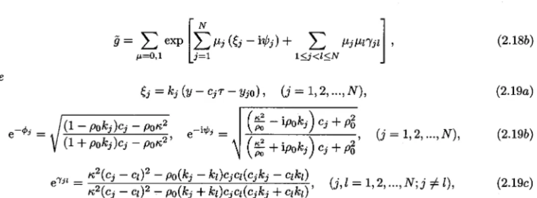
Figure

1

_plots

_{the velocities c+} \equiv _{c_{j}}

($\epsilon$_{j} = +1)

and c_{-} \equiv

c_{j}($\epsilon$_{j} = -1)

as afunction of

$\rho$_{0}k

\equiv

_{$\rho$_{0}k_{j}.}

The

_velocity

\mathrm{c}_{+} is

positive

for 0 <

_{$\rho$_{0}k}

< 1 and

_negative

for 1<

_{$\rho$_{0}k}

<

\sqrt{$\kappa$^{4}+p_{0}^{2}}/$\rho$_{0}

. Itexhibits the

singularity

at

_{$\rho$_{\mathrm{O}}k=1}

.

Specifically,

$\rho$_{0}($\kappa$^{2}+\sqrt{$\kappa$^{4}+$\rho$_{0}^{2}}<c+<\infty, (0<$\rho$_{0}k<1) , (2.23a)

$\rho$_{0}k

Figure

1.The

_{velocity c=c\pm \mathrm{o}\mathrm{f}}

the solitonas afunction of

_{$\rho$_{0}k}

for

_{$\rho$_{0}=1}

and $\kappa$=1: _{c_{+}}

(solid curve),

c_{-}

(dashed curve).

On the other

_hand,

the

_velocity

c_{-}isacontinuousfunction of

_{$\rho$_{0}k}

and takes

_negative

valuesinthe interval

(2.23),

asindicated

_by

the

_inequality

‐

\displaystyle \frac{$\rho$_{0}^{3}}{$\kappa$^{2}}<c_{-}<-$\rho$_{0}(\sqrt{$\kappa$^{4}+$\rho$_{0}^{2}}-$\kappa$^{2})

,

(0<$\rho$_{0}k<\sqrt{$\kappa$^{4}+$\rho$_{0}^{2}}/ $\rho$ 0)

.

(2.24)

In

particular,

c_{-} =

-$\rho$_{0}^{3}/(2$\kappa$^{3})

at

$\rho$_{0}k=

1. It turns outthat the soliton with the

velocity

c_{-}

always

propagatestothe left whereas the soliton with the

_velocity

_c+propagatestothe

_right

and left

_depending

onthe value of

p_{0}k

.

Thus,

the two‐soliton solution exhibits both the

overtaking

and head‐on collisions.

Using

(2.21),

the_expressions

_(2.19b)

become

\displaystyle \mathrm{e}^{-$\phi$_{j}}=\frac{|(1-$\rho$_{0}k_{j})c_{j}-$\rho$_{0}$\kappa$^{2}|}{ $\rho$ 0\sqrt{$\kappa$^{4}+$\rho$_{0}^{2}}}=\frac{\{(1-$\rho$_{0}k_{j})c_{j}-p_{0}$\kappa$^{2}\}\mathrm{s}\mathrm{g}\mathrm{n}c_{j}}{ $\rho$ 0\sqrt{$\kappa$^{4}+$\rho$_{0}^{2}}}

,

\displaystyle \mathrm{e}^{-\mathrm{i}$\psi$_{j}}=\frac{$\kappa$^{2}c_{j}+$\rho$_{0}^{3}-\mathrm{i}$\rho$_{0}^{2}k_{\mathrm{j}}c_{j}}{\sqrt{$\kappa$^{4}+$\rho$_{0}^{2}}|c_{j}|}

,

(2.25)

wherethe

_symbol

_{sgn denotes the}

_sign

function. Inview of the relation

_{d_{j}^{2}-d_{l}^{2}=$\rho$_{0}^{4}(-k_{\mathrm{j}}^{2}+k_{l}^{2})}

which

follows from

_(2.21b)

,theexpression

(2.19c)

becomes

\displaystyle \mathrm{e}^{$\gamma$_{jl}}=\frac{(d_{j}-d_{l})^{2}+$\rho$_{0}^{4}(k_{j}-k_{l})^{2}}{(d_{j}-d_{l})^{2}+$\rho$_{0}^{4}(k_{j}+k_{l})^{2}}

.

(2.26)

3.

_Properties

of soliton solutions

In this _section,wefirst

explore

the

_properties

of the one‐soliton solutionindetail and then

perform

an

_asymptotic

analysis

of the

general

N‐soliton solution.

Consequently,

the formula for the

phase

shift

of each sohton will be derived. The {wo‐solitoncaseisdiscussed

shortly.

3.1. One‐soliton solution

The tau‐functions

corresponding

tothe one‐soliton solutionare

_{given by}

(2.17)

and

(2.18)

with N=1

f=1+\mathrm{e}^{ $\xi$+ $\phi$}, \tilde{f}=1+\mathrm{e}^{ $\xi$- $\phi$}

,

(3.1)

with

$\xi$=k(y-c $\tau$-y_{0}) , c=c\displaystyle \pm=\frac{p_{0}^{3}}{\pm\sqrt{$\kappa$^{4}+$\rho$_{0}^{2}-$\rho$_{0}^{4}k^{2}}-$\kappa$^{2}}, (3.3a)

\displaystyle \mathrm{e}^{- $\phi$}=\frac{|(1-$\rho$_{0}^{ $\iota$}k)c-$\rho$_{0}$\kappa$^{2}|}{$\rho$_{0}\sqrt{$\kappa$^{4}+$\rho$_{0}^{2}}}, \mathrm{e}^{-\mathrm{i} $\psi$}=\frac{$\kappa$^{2}c+$\rho$_{0}^{3}-\mathrm{i}$\rho$_{0}^{2}kc}{\sqrt{$\kappa$^{4}+$\rho$_{0}^{2}}|c|}, (3.3b)

wherewehave_put

$\xi$=$\xi$_{1}, k=k_{1},

c=c_{1},

$\phi$=$\phi$_{1}, $\psi$=$\psi$_{1}

andy_{0}=y_{10}for

simplicity.

The

_{parametric representation}

of the one‐soliton solution is obtained

by introducing

(3.1)

and

_(3.2)

with

_(3.3)

into

_(2.15).

Itcanbewritten inthe form

u=\displaystyle \frac{kc\sinh $\phi$}{\cosh $\xi$+\cosh $\phi$}, p=$\rho$_{0}+\frac{kc\sin $\psi$}{\cosh $\xi$+\cos $\psi$}, (3.4a)

X\displaystyle \equiv x-\tilde{c}t-x_{0}=\frac{ $\xi$}{$\rho$_{0}k}+\ln\frac{1-\mathrm{t}\Re \mathrm{A}_{2}^{4}\mathrm{t}\Re \mathrm{A}_{2}^{ $\xi$}}{1+\mathrm{t}_{\partial \mathrm{J}}\mathrm{A}_{2}^{4}\mathrm{t}\Re \mathrm{A}_{2}^{ $\xi$}}, (3.4b)

with

\displaystyle \sinh $\phi$=\frac{k|c|}{\sqrt{$\kappa$^{4}+$\rho$_{0}^{2}}}

,

\cosh $\phi$=\sqrt{1+\frac{k^{2}c^{2}}{$\kappa$^{4}+$\rho$_{0}^{2}}},

\displaystyle \sin $\psi$=\frac{$\rho$_{0}^{2}kc}{\sqrt{$\kappa$^{4}+$\rho$_{0}^{2}}|c|}

,

\displaystyle \cos $\psi$=\frac{$\kappa$^{2}c+$\rho$_{0}^{3}}{\sqrt{$\kappa$^{4}+$\rho$_{0}^{2}}|c|}

,

(3.4c)

where

_{\tilde{c}=c/p_{0}}

is the

_velocity

of the solitoninthe

_{(x, t)}

coordinate_system,

_{x_{0}=y_{0}/ $\kappa$}

and theconstant

din

_(2.15b)

has been chosen such that

_{$\xi$=0 corresponds}

toX=0. Letus nowdescribesome

important

propertiesof the solution.

(a)

Smoothness

_of

the solution

We_computetheyderivative ofxfrom

(3.4b)

toobtain

x_{y}=\displaystyle \frac{1}{$\rho$_{0}}-\frac{k\sinh $\phi$}{\cosh $\xi$+\cosh $\phi$}

.

(3.5)

Since k>0 and

$\phi$>0,

x_{y}\geq x_{y}|_{ $\xi$=0}

.

Using

(3.3b)

for

$\phi$ gives

x_{y}|_{ $\xi$=0}=\displaystyle \frac{1}{$\rho$_{0}}(1-$\rho$_{0}k\mathrm{t}\mathrm{u}\mathrm{A}\frac{ $\phi$}{2}) =\frac{1}{|c|}(\sqrt{$\rho$_{0}^{2}+$\kappa$^{4}}-$\kappa$^{2})

.

(3.6)

Thus,

ifcis

_finite,

_{then x_{y} >0} , and themap

(2.1)

becomesone‐to‐one,

assuring

that the solutionis

smooth and

_{nonsingular. Actually,}

one canshow that the derivatives

du/dX

and

d $\rho$/dX

arefinite for

arbitrary

X\in \mathbb{R}.

(b)

Amplitude‐velocity

relation

The

_{amplitude‐velocity}

relation of the solitonis an_important characteristic of thewave. Itcanbe

derived

_simply

from the

_explicit

form of the solution. To this

_end,

let

_{A_{ $\rho$}}

be the

_amplitude

of thewave

measured from the constant level_p =

$\rho$_{0} and

A_{u}

be that of the fluid

velocity, namely

A_{ $\rho$}

=

$\rho$(X

=

0)-$\rho$_{0}, A_{u}=|u(X=0

It follows from

_(3.3)

and

_(3.4)

that

A_{ $\rho$}=(\sqrt{$\kappa$^{4}+$\rho$_{0}^{2}}|\tilde{c}|-$\kappa$^{2}\tilde{c}-$\rho$_{0}^{2})/$\rho$_{0}\rangle A_{u}=||\tilde{c}-$\kappa$^{2}|-\sqrt{$\kappa$^{4}+$\rho$_{0}^{2}}|

,

(3.7)

where

_{\tilde{c}=c/p_{0}}

. Notefrom

(3.3b)

and

(3.4a)

that

2 1.5 1 0.5

0-10

-5 0 5 10 X 3 2 1 0

-1-10 -5 0 5 10

X -10 -5 0 5 10 X

Figure

2.One‐soliton solution. u: thin solid_{curve, $\rho$}: bold solidcurve. a:

$\kappa$=1, $\rho$_{0}=1, k=0.4,

\tilde{c}=

\tilde{c}+=2.81,

\mathrm{b}: $\kappa$=1,

$\rho$_{0}=1, k=1.0, \tilde{c}=\tilde{\mathrm{c}}+=-1.25.

’\mathrm{c}:

$\kappa$=1, $\rho$_{0}=1, k=1.4,

\tilde{c}=\tilde{c}_{-}=-0.83.

Invoking

the_expressionof the

_velocity

cfrom

(3.3a)

, we can seethat

A_{ $\rho$}

>0for

arbitrary

c=c\pm

whereas

_u(X=0)>0

for c>0 and

_u(X=0)<0

for c<0. These results show that the

profile

of $\rho$is

always

of

_bright

_type,but that of u

depends

onthe

_propagation

direction of the soliton.

Actually,

ifcis

positive

(negative),

thenuiscurved

upward

(downward).

Figure

2

_depicts

the

_{typical profile}

ofuand _$\rho$for the

_{right‐going}

soliton

(a),

and the

_left‐going

soliton

(b)

and

_(c),

_{respectively.}

3.2. N‐soliton solution

Here,

we

_investigate

the

_asymptotic

behavior of the N‐soliton solution for

_large

time. Let

_{\tilde{c}_{n}(=}

c_{n}/$\rho$_{0} (n=1,2, \ldots, N)

Ue the

_velocity

of the nthe solitoninthe

_{(x, t)}

coordinate_system,and order them

inaccordance with the relation\tilde{c}_{N}<\tilde{c}_{N-1}< <\tilde{c}_{1}. We take the hmit t\rightarrow-\inftywith the

phase

variable

$\xi$_{n}

of the nth soliton

_being

fixed.

_Then,

the other

_phase

variables behave hke

_{$\xi$_{1}, $\xi$_{2},}

_{$\xi$_{n-1}\rightarrow+\infty}

,and

$\xi$_{n+1},$\xi$_{n+2},

$\xi$_{N}\rightarrow-\infty

.

Performing

an

asymptotic

analysis

for the tau‐functions

(2.17)

and

(2.18)

and

substituting

the

_{leading‐order approximations}

for them into

_(2.15),

weobtain the

_asymptotic

form of _u,

$\rho$and x

u\displaystyle \sim\frac{k_{n}\mathrm{c}_{n}\sinh$\phi$_{n}}{\cosh($\xi$_{n}+$\delta$_{n}^{(-)})+\cosh$\phi$_{n}}, p\sim p_{0}+\frac{k_{n}c_{n}\mathrm{s}\dot{\mathrm{m}}$\psi$_{n}}{\cosh($\xi$_{n}+$\delta$_{n}^{(-)})+\cos$\psi$_{n}}

,

(3.8)

x-\displaystyle \tilde{c}_{n}t-x_{n0}\sim\frac{$\xi$_{n}}{$\rho$_{0}k_{n}}+\ln\frac{1-\mathrm{t}\mathrm{a}\mathrm{M}_{2}^{\mathrm{g}_{n}}\tanh\frac{($\xi$_{n}+$\delta$_{n}^{\text{（-})})}{2}}{1+\mathrm{t}\mathrm{a}\mathrm{J}\mathrm{A}_{2}^{4}\underline{n}\mathrm{t}\mathrm{a}\mathrm{J}\mathrm{A}\frac{($\xi$_{n}+$\delta$_{n}^{\text{（-})})}{2}}-2\sum_{j=1}^{n-1}$\phi$_{j}

,

(3.9)

where

$\delta$_{n} =\displaystyle \sum_{j=1}^{n-1}$\gamma$_{nj}=\sum_{j=1}^{n-1}\ln[\frac{(\acute{d}_{n}-d_{j})^{2}+$\rho$_{0}^{4}(k_{n}-k_{j})^{2}}{(d_{n}-d_{j})^{2}+$\rho$_{0}^{4}(k_{n}+k_{j})^{2}}]

.

(3.10)

+\infty.

Applying

the similar

analysis yields

the

asymptotic

forms

corresponding

to

(3.8)

and

(3.9)

u\displaystyle \sim\frac{k_{n}c_{n}\sinh$\phi$_{n}}{\cosh($\xi$_{n}+$\delta$_{n}^{(+)})+\cosh$\phi$_{n}}, $\rho$\sim$\rho$_{0}+\frac{k_{n}c_{n}\sin$\psi$_{n}}{\cosh($\xi$_{n}+$\delta$_{n}^{(+)})+\cos$\psi$_{n}}

,

(3.11)

x-\displaystyle \tilde{c}_{ $\eta$}t-x_{n0}\sim\frac{$\xi$_{n}}{$\rho$_{0}k_{n}}+\ln\frac{1-\tanh_{2}^{$\mu$_{n}}\tanh\frac{($\xi$_{n}+$\delta$_{n}^{\text{（}+)})}{2}}{1+\mathrm{t}\mathrm{m}\mathrm{h}_{2}^{\mathrm{A}}n-\mathrm{t}\Re \mathrm{A}\frac{($\xi$_{n}+$\delta$_{n}^{(+)})}{2}}-2\sum_{j=1}^{n-1}$\phi$_{\hat{J}\rangle}

(3.12)

where

$\delta$_{n}^{(+)}=\displaystyle \sum_{j=n+1}^{N}$\gamma$_{nj}=\sum_{j=n+1}^{N}\ln[\frac{(d_{n}-d_{j})^{2}+$\rho$_{0}^{4}(k_{n}-k_{j})^{2}}{(d_{n}-d_{j})^{2}+$\rho$_{0}^{4}(k_{n}+k_{\mathrm{j}})^{2}}]

.

(3.13)

These results show that as t \rightarrow \pm\infty_, the N‐soliton solution is a

_{superposition}

of N

independent

solitons each of which has the form

_given

_by

_(3.4).

Theneteffect of the collision of solitonsappearsas a

phase

shift. Tosee

this,

letx_{nc}Ue thecenter

position

of the nth soliton. It then follows from

_(3.9)

and

(3.12)

that the

_trajectory

ofx_{nc}is

_{given by}

x_{n\mathrm{c}}\displaystyle \sim\tilde{\mathrm{c}}_{n}t-\frac{$\delta$_{n}^{(-)}}{$\rho$_{0}k_{n}}-2\sum_{j=1}^{n-1}$\phi$_{j},

(t\rightarrow-\infty)

,

x_{n\mathrm{c}}\displaystyle \sim\tilde{c}_{n}t-\frac{$\delta$_{n}^{\mathrm{t}+)}}{$\rho$_{0}k_{n}}-2\sum_{j=n+1}^{N}$\phi$_{j},

(t\rightarrow+\infty)

.

(3.14)

We define the

_phase

shift of the nth soliton which_propagatestothe

_{right by}

_{$\Delta$_{n}^{R}=x_{n\mathrm{c}}(t\rightarrow+\infty)-x_{nc}(t\rightarrow}

-\infty)

, and thatpropagatestothe left

by

$\Delta$_{n}^{L} =x_{nc}(t\rightarrow -\infty)-x_{nc}(t\rightarrow+\infty)

.

Using

(2.19b)

_,

(3.10),

(3.13)

and

_(3.14),

wefind that

$\Delta$_{n}^{R}=\displaystyle \frac{1}{$\rho$_{0}k_{n}} [\sum_{j=1}^{n-1}\ln[\frac{(d_{n}-d_{j}\rangle^{2}+p_{0}^{4}(k_{n}-k_{j})^{2}}{(d_{n}-d_{j})^{2}+$\rho$_{0}^{4}(k_{n}+k_{j})^{2}}] -\sum_{j=n+1}^{N}\ln[\frac{(d_{n}-d_{j})^{2}+$\rho$_{0}^{4}(k_{n}-k_{j})^{2}}{(d_{n}-d_{j})^{2}+$\rho$_{0}^{4}(k_{n}+k_{j})^{2}}]]

+\displaystyle \sum_{j=n+1}^{N}

\mathrm{I}\mathrm{n}

[\displaystyle \frac{(1-$\rho$_{0}k_{j})\tilde{c}_{j}-$\kappa$^{2}}{(1+$\rho$_{0}k_{j})\tilde{c}_{j}-$\kappa$^{2}}]

_{-\displaystyle \sum_{j=1}^{n-1}]_{\mathrm{J}\mathrm{J}}[\frac{(1-$\rho$_{0}k_{j})\tilde{c}_{j}-\dot{ $\kappa$}^{2}}{(1+$\rho$_{0}k_{j})\tilde{c}_{j}-$\kappa$^{2}}]}

.

(3.15)

The_expressionof

_{$\Delta$_{n}^{L}}

is

equal

to

_{-$\Delta$_{n}^{R}.}

3.3. Two‐soliton solution

The twesoliton solutionisthemostfundamental elementin

_{understanding}

the

_dynamics

of solitons

since each soliton exhibits _pair‐wise interactions with every other soliton. There exist two types of

interactionsfor the CH2

equation,

i.e.,the

_overtaking

and head‐on collisions.

The tau‐functions for the two‐soliton solutionare

given by

(2.17), (2.18)

and

(2.19)

with N=2.

They

read

f=1+\mathrm{e}^{$\xi$_{1}+$\phi$_{1}}+\mathrm{e}^{$\xi$_{2}+$\phi$_{2}}+ $\delta$ \mathrm{e}^{$\xi$_{1}+$\xi$_{2}+$\phi$_{1}+$\phi$_{2}}, \tilde{f}=1+\mathrm{e}^{$\xi$_{1}-$\phi$_{1}}+\mathrm{e}^{$\xi$_{2}-$\phi$_{2}}+ $\delta$ \mathrm{e}^{$\xi$_{1}+$\xi$_{2}-$\phi$_{1}-$\phi$_{2}}

,

(3.16)

g=1+\mathrm{e}^{$\xi$_{1}+\mathrm{i}$\psi$_{1}}+\mathrm{e}^{$\xi$_{2}+\mathrm{i}$\psi$_{2}}+ $\delta$ \mathrm{e}^{$\xi$_{1}+$\xi$_{2}+\mathrm{i}$\psi$_{1}+\mathrm{i}$\psi$_{2}}, \tilde{g}=1+\mathrm{e}^{$\xi$_{1}-\mathrm{i}$\psi$_{1}}+\mathrm{e}^{$\xi$_{2}-\mathrm{i}$\psi$_{2}}+ $\delta$ \mathrm{e}^{$\xi$_{1}+$\xi$_{2}-\mathrm{i}$\psi$_{1}-\mathrm{i}$\psi$_{2}}

,

(3.17)

where

$\xi$_{j}=k_{j}(y-c_{j} $\tau$-y_{j0}) , (j=1,2) , (3.18a)

$\delta$=\displaystyle \mathrm{e}^{$\gamma$_{12}}=\frac{(d_{1}-d_{2})^{2}+$\rho$_{0}^{4}(k_{1}-k_{2})^{2}}{(d_{1}-d_{2})^{2}+$\rho$_{0}^{4}(k_{1}+k_{2})^{2}}, (3.18b)

4 3 2 1

0‐{

4 3 2 \uparrow

\underline{0}.

Figure

3. The

_overtaking

collision oftwosolitons. u: thin solid_{curve, $\rho$}: bold solidcurve.

_$\kappa$=1,

_{$\rho$_{0}=}

1,

k_{1}=0.8, k_{2}=0.7, \tilde{c}_{1+}=6.02, \tilde{\mathrm{c}}_{2+}=4.37.

\mathrm{e}^{-$\phi$_{j}}=\sqrt{\frac{(1-$\rho$_{0}k_{j})c_{j}-$\rho$_{0}$\kappa$^{2}}{(1+$\rho$_{0}k_{j})c_{j}-$\rho$_{0}$\kappa$^{2}}},

\mathrm{e}^{-\mathrm{i}$\psi$_{j}}=\sqrt{\frac{(\frac{$\kappa$^{2}}{ $\rho$ 0}-\mathrm{i}$\rho$_{0}k_{j})c_{j}+$\rho$_{0}^{2}}{(\frac{$\kappa$^{2}}{ $\rho$ 0}+\mathrm{i}$\rho$_{0}k_{j})c_{j}+$\rho$_{0}^{2}}},

(j=1,2)

.

(3.18c)

Recall from

_(2.21)

that the

_velocity

of

_jth

sohtonin

_{(x_{\rangle}t)}

coodinate_systemis

_given

_by

\displaystyle \tilde{c}_{j}=c_{j}/$\rho$_{0}=\frac{p_{0}^{2}}{d_{j}-$\kappa$^{2}}, d_{j}=$\epsilon$_{j}\sqrt{$\kappa$^{4}+$\rho$_{0}^{2}-$\rho$_{0}^{4}k_{j}^{2}}, (j=1,2)

.

(3.19)

Substituting

(3.16)

and

_(3.17)

into

_(2.15),

we obtain the _{parametric representation}of the twQsoliton

solution. Asseenfrom

_{Figure 1,}

this solution describes both the

_overtaking

and headon

_collisions,

which

aretreated

_separately.

(a)

Overtaking

collision

We consider thecase_{c_{j}=c_{j+},}

0<$\rho$_{0}k_{j}<1

sothat

_{0<\tilde{c}_{2+}<\tilde{c}_{1+}}

.

Figure

3illustrates the

overtaking

collision oftwosolution for four distinct values oft. The solitonic feature of the solutionisobvious from

the

_figure

which confirmsan

_asymptotic

_{analysis presented}

in

_§3.1.

The

_phase

shift of each solitonis

given

by

(3.15).

Explicitly,

$\Delta$_{1}^{R}=-\displaystyle \frac{1}{$\rho$_{0}k_{1}}\ln [\frac{(d_{1}-d_{2})^{2}+$\rho$_{0}^{4}(k_{1}-k_{2})^{2}}{(d_{1}-d_{2})^{2}+$\rho$_{0}^{4}(k_{1}+k_{2})^{2}}] +\ln [\frac{(1-$\rho$_{0}k_{2})\tilde{c}_{2}-$\kappa$^{2}}{(1+$\rho$_{0}k_{2})\tilde{\mathrm{c}}_{2}-$\kappa$^{2}}] (3.20a)

$\Delta$_{2}^{R}=\displaystyle \frac{1}{$\rho$_{0}k_{2}}\ln [\frac{(d_{1}-d_{2})^{2}+$\rho$_{0}^{4}(k_{1}-k_{2})^{2}}{(d_{1}-d_{2})^{2}+$\rho$_{0}^{4}(k_{1}+k_{2})^{2}}] -\ln [\frac{(1-$\rho$_{0}k_{1})\tilde{c}_{1}-$\kappa$^{2}}{(1+p_{0}k_{1})\tilde{c}_{1}-$\kappa$^{2}}] , (3.20b)

with

8 6 4 2 0

-\underline{2}_{\mathrm{J}, $\iota$}

X 8 6 4 2 0 -2 X X X

Figure

4. The head‐on collision oftwosolitons. u: thin solid_{curve, $\rho$}: bold solidcurve. $\kappa$= _{1,p_{0}=}

1,

k_{1}=0.8, k_{2}=0.7, \tilde{c}_{1+}=6.02, \tilde{c}_{2+}=-1.25

(b)

Head‐on collision

An

_example

of the head‐on colhsionisshownin

_Figure

_4,

where the

_velocity

of each soliton is chosen

asc_{2+} < 0 < _{c_{1+}}. The formula of the

phase

shift for the

right‐running

soliton is the same as

(3.20a)

whereas that of the

left‐running

solitonis

_given

_by

_{$\Delta$_{2}^{L}=-$\Delta$_{2}^{R}.}

4. Reductionstothe Camassa‐Holm and

two‐component

Hunter‐Saxton

_equations

Inthissection,wefirst show that the CH2

_equation

anditsN‐soliton solution reducetothose of the CH_equation

_by

meansofan

_appropriate

_{limiting procedure. Then,}

wedemonstrate that the short‐wave

limit of the CH2_equation

_yields

the_{two‐component}Hunter‐Saxton

_equation.

4.1.

Reductiontothe Camassa‐Holm

_equation

The CH

_equation

_(1.3)

isderived

_simply

from the CH2

_equation

_{by putting $\rho$=0}

. In this

setting,

one

must

_impose

the

_boundary

condition

_{$\rho$_{0}=0}

. TheN‐sohton solution of the CH

equation

isreduced from

that of the CH2_equation

_{by taking}

the limit

_{$\rho$_{0}\rightarrow 0}

. Toshow

this,

weintroduce tha

following scaling

variables

u=\displaystyle \overline{u}, $\rho$= $\rho$ 0\overline{ $\rho$}, m=\overline{m}, x=\overline{x}, y=\frac{p_{0}}{ $\kappa$}\overline{y}, t=\overline{t}, $\tau$=\overline{ $\tau$}, d=\overline{d},

k_{j}=\displaystyle \frac{ $\kappa$}{$\rho$_{0}}\overline{k}_{j}, \mathrm{c}_{j}=\frac{$\rho$_{0}}{ $\kappa$}\overline{c}_{j}, y_{j0}=\frac{$\rho$_{0}}{ $\kappa$}\overline{y}_{j0}, (j=1,2, \ldots, N)

.

(4.1)

Then,

the

_{leading‐order asymptotics}

_{of c_{j} from}

_(2.21)

and

_{$\phi$_{\mathrm{j}}, $\psi$_{j}}

_{and $\gamma$_{\mathrm{j}l} from}

_{(2.19b, c)}

arefoundtobe

c_{j}\displaystyle \sim\frac{2$\rho$_{0}$\kappa$^{2}}{1-( $\kappa$\overline{k}_{j})^{2}}, (j=1,2, \ldots, N) , (4.2a)

\displaystyle \mathrm{e}^{-$\phi$_{j}}\sim\frac{1- $\kappa$\overline{k}_{j}}{1+ $\kappa$\overline{k}_{\mathrm{j}}}\equiv \mathrm{e}^{-\overline{ $\phi$}_{j}}, \mathrm{e}^{-\mathrm{i}$\psi$_{j}}\sim 1-\frac{$\rho$_{0}}{ $\kappa$}\overline{k}_{j}, (j=1,2, \ldots,N) , (4.2b)

\mathrm{e}^{$\gamma$_{j1}}=

(\displaystyle \frac{\overline{k}_{j}-\overline{k}_{l}}{\overline{k}_{\hat{J}}+\overline{k}_{l}})^{2}\equiv \mathrm{e}^{\overline{ $\gamma$}_{j1}}, (j, l=1,2, \ldots, N;j\neq l)

.

(4.2c)

We notethat a

_limiting

form

_{\overline{\mathrm{c}}_{j}}

\sim

-$\rho$_{0}^{2}/(2 $\kappa$)

whicharises from

(2.21)

with $\epsilon$_{\mathrm{j}} =

-1(j = 1,2)

isnot

relevantsincethisexpression

degenerates

tozero as

p_{0}\rightarrow 0.

The

_asymptotics

of the tau‐functions

_f

and

_\tilde{f}

from

_(2.17)

andgand

\tilde{g}

from

_(2.18)

become

f\displaystyle \sim\sum_{ $\mu$=0,1}\exp [\sum_{j=1}^{N}$\mu$_{j}(\overline{ $\xi$}_{j}+\overline{ $\phi$}_{j})+\sum_{1\leq j<l\leq N}$\mu$_{j}$\mu$_{l}\overline{ $\gamma$}_{j} $\iota$] \equiv\overline{f}, (4.3a)

\displaystyle \tilde{f}\sim\sum_{ $\mu$=0,1}\exp [\sum_{j=1}^{N}$\mu$_{\mathrm{j}}(\overline{ $\xi$}_{j}-\overline{ $\phi$}_{j})+\sum_{1\leq j<l\leq N}$\mu$_{j}$\mu$_{l}\overline{ $\gamma$}_{j}i] \equiv f (4.3b)

g=\displaystyle \overline{f}_{0}+\mathrm{i}\frac{$\rho$_{0}}{ $\kappa$}\overline{f}_{0,\overline{y}}+O($\rho$_{0}^{2}) , \tilde{g}=\overline{f}_{0}-\mathrm{i}\frac{$\rho$_{0}}{ $\kappa$}\overline{f}_{0,\overline{y}}+O($\rho$_{0}^{2})

,

(4.4)

where

\displaystyle \overline{f}_{0}=\sum_{ $\mu$=0,1}\exp [\sum_{j=1}^{N}$\mu$_{j}\overline{ $\xi$}_{j}+\sum_{1\leq j< $\iota$\leq N}$\mu$_{j}$\mu$_{l}\overline{ $\gamma$}_{jt}] , (4.5a)

\overline{ $\xi$}_{j}=\overline{k}_{\mathrm{j}}(\overline{y}-\overline{c}_{j}\overline{ $\tau$}-\overline{y}_{j0})

,

\displaystyle \overline{c}_{j}=\frac{2$\kappa$^{3}}{1-( $\kappa$\overline{k}_{j})^{2}}, (j=1,2, \ldots, N)

.

(4.5b)

Introducing

(4.3)

and

_(4.4)

into

_(2.15),

weobtain the

limiting

forms of_{u, $\rho$}and x

\displaystyle \overline{u}= (\ln\frac{\overline{\tilde{f}}}{\overline{f}})_{\overline{ $\tau$}} $\rho$\sim$\rho$_{0}(1-\frac{2}{ $\kappa$}(\ln\overline{f}_{0})_{\overline{y} $\tau$}) \equiv p_{0}\overline{ $\rho$}, (4.6a)

あ

=\displaystyle \frac{\overline{y}}{ $\kappa$}+1_{\mathrm{J}\mathrm{J}}\frac{\sim_{f}^{\sim}}{\overline{f}}+\overline{d}.

_(4.6b)

The_{parametric representation}of the N‐sohton solutiongiven

by

(4.6)

with the tau‐functions

_(4.3)

coincides

_perfectly

with that of the CHequationpresentedin

_[6].

In

_particular,

the one‐soliton solution

(3.4)

reducesto

\displaystyle \overline{u}=\frac{2 $\kappa$\overline{c}\overline{k}^{2}}{1+$\kappa$^{2}\overline{k}^{2}+(1-$\kappa$^{2}\overline{k}^{2})\cosh\overline{ $\xi$}}, (4.7a)

\displaystyle \overline{X}=\overline{x}-c \overline{x}_{0}= \frac{\overline{ $\xi$}}{ $\kappa$\overline{k}}+\mathfrak{l}\mathrm{n}\frac{(1- $\kappa$\overline{k})\mathrm{e}^{\overline{ $\xi$}}+1+ $\kappa$\overline{k}}{(1+ $\kappa$\overline{k})\mathrm{e}^{\overline{ $\xi$}}+1- $\kappa$\overline{k}}, (4.7b)

with

\overline{ $\xi$}=\overline{k}

(

\overline{y}-

③テー90)

\displaystyle \overline{c}=\frac{2$\kappa$^{3}}{1-( $\kappa$\overline{k})^{2}},

\overline{\tilde{c}}=\overline{c}/ $\kappa$,

(4.7c)

reproducing

the one‐sohton solution of the CH_equation.

Thelimitingform of thephaseshift which is denoted

by

\overline{ $\Delta$}_{n}^{R}

canbe obtainedby

applying

the

scalings

(4.1)

to

_(3.15)

andusing

_(4.1)

and

_(4.2a),

resultingin

+\displaystyle \sum_{j=n+1}^{N}\ln(\frac{1- $\kappa$ k_{\mathrm{j}}}{1+ $\kappa$ k_{j}})^{2}-\sum_{j=1}^{n-1}\mathrm{I}_{\mathrm{J}1}(\frac{1- $\kappa$ k_{j}}{1+ $\kappa$ k_{j}})^{2} (n=1,2, \ldots,N)

.

(4.8)

This coincides with the formula for the

_phase

shift of the nth soliton which has been derive for the

N‐soliton solution of the CH

_equation

_[6].

Remark 4.1.

Ifwe_put

\overline{r}=\mathrm{K}-2(\ln\overline{f}_{0})_{\overline{y} $\tau$}

,then

\overline{m}=\overline{r}^{2}, \overline{ $\rho$}=\overline{r}/ $\kappa$

.

(4.9)

The

_reciprocal

transformation

_(2.1a)

_reproduces

the

_{corresponding}

onefor the CH_equation

d\overline{y}=\overline{r}d\overline{x}-\overline{r}\overline{u}d\overline{t}

, dテ=d\overline{t}.

(4.10)

The bilinear

_equations

_{(2.10)‐(2.12)}

_reduce,

inthe

_{scaling limit,}

tothe bilinear

equations

$\kappa$ D_{\overline{y}}\overline{\tilde{f}}\cdot\overline{f}+\overline{\tilde{f}}\overline{f}-f_{0}^{2}=0

,

(4.11)

Dテ

D_{\overline{y}}\overline{f}_{0}\cdot\overline{f}_{0}+ $\kappa$(\overline{\tilde{f}}\overline{f}-\overline{f}_{0}^{2})=0

,

(4.12)

$\kappa$ D_{\overline{ $\tau$}}Dす

\overline{\tilde{f}}\cdot\overline{f}+D_{\overline{ $\tau$}}\overline{\tilde{f}}\cdot\overline{f}+$\kappa$^{3}D_{\overline{y}}\sim_{f}^{\sim}\cdot\overline{f}=0

,

(4.13)

whereas the

_scaling

limit of

_(2.13)

isshowntocoincide with

_(4.11).

Onecanshow that the tau‐functions

\overline{f}

and

\overline{\tilde{f}}

from

_(4.3)

and

_{\overline{f}_{0}}

from

_(4.5)

solve the above bilinear

_equations.

4.2.

Reductiontothe_{two‐component}Hunter‐Scwton

_equation

The_{two‐component}Hunter‐Saxton

_(HS2)

_equationstemsfrom the short‐wave limit of the CH2equa‐

tion. To show

_this,

weintroduce the

scaling

variables

u=$\epsilon$^{2}\displaystyle \hat{u}, $\rho$= $\epsilon$\hat{p}, m=\hat{m}, x= $\epsilon$\hat{x}, y=$\epsilon$^{2}\hat{y}, t=\frac{\hat{t}}{ $\epsilon$}, $\tau$=\frac{\hat{ $\tau$}}{ $\epsilon$}

.

(4.14)

Rescaling

the CH2equation

(1.1)

by

(4.14)

and

_taking

the limit $\epsilon$\rightarrow 0,weobtain the HS2

equation

\hat{m}_t+ûm免\hat{x}+2\hat{m}û￡十

\hat{ $\rho$}\hat{p}_{\hat{x}}=0,

\hat{ $\rho$}_{\hat{t}}+(\hat{p}\hat{u})

￠ =0,

(4.15)

where \hat{m}=

−ûx

\hat{}

x\hat{}+ $\kappa$2. The N‐sohton solution of the HS2equationcanbe reduced from that of the CH2

equation

by

meansofa

limiting procedure.

Th_appropriate

scaling

variablearefoundtobe

k_{j}=\displaystyle \frac{\hat{k}_{j}}{$\epsilon$^{2}} , c_{j}=$\epsilon$^{3}\hat{c}_{j}, y_{j0}=$\epsilon$^{2}\overline{y}_{j0}, (j=1,2, \ldots, N) , $\rho$_{0}= $\epsilon$\hat{ $\rho$}_{0}, d= $\epsilon$\hat{d}

.

(4.16)

Inthe limit $\epsilon$\rightarrow 0, the solitonparameters

corresponding

tothose

given by

(4.2)

have the

leading‐order

asymptotics

c_{j}\displaystyle \sim-\frac{$\epsilon$^{3}}{\hat{ $\rho$}_{0}\hat{k}_{j}^{2}}($\kappa$^{2}+\hat{d}_{j}) , \hat{d}_{j}= $\epsilon$ j\sqrt{$\kappa$^{4}-\hat{ $\rho$}_{0}^{4}\hat{k}_{j}^{2}}, (j=1,2, \ldots, N) , (4.17a)

\displaystyle \mathrm{e}^{-$\phi$_{j}} \sim 1+ $\epsilon$\frac{\hat{k}_{j}\hat{c}_{j}}{$\kappa$^{2}}, \mathrm{e}^{-\mathrm{i}$\psi$_{j}}\sim\sqrt{\frac{(\frac{$\kappa$^{2}}{\hat{ $\rho$}0}-\mathrm{i}\hat{ $\rho$}_{0}\hat{k}_{j})\hat{c}_{j}+\hat{p}_{0}^{2}}{(\frac{$\kappa$^{2}}{\hat{ $\rho$}0}+\mathrm{i}\hat{ $\rho$}_{0}\hat{k}_{j})\hat{c}_{j}+\hat{ $\rho$}_{0}^{2}}}\equiv \mathrm{e}^{-\mathrm{i}\hat{ $\psi$}_{j}}, (j=1,2, \ldots, N) , (4.17b)

The tau‐functions

_(2.17)

and

_(2.18)

have the

_{leading‐order asymptotics}

f\displaystyle \sim\hat{f}+\frac{ $\epsilon$}{$\kappa$^{2}}\hat{f}_{\hat{ $\tau$}}, \tilde{f}\sim\hat{f}-\frac{ $\epsilon$}{$\kappa$^{2}}\hat{f}_{\hat{ $\tau$}}

,

(4.18)

g\displaystyle \sim\sum_{ $\mu$=0,1}\exp[\sum_{j=1}^{N}$\mu$_{j}(\hat{ $\xi$}_{\mathrm{j}}+\mathrm{i}\hat{ $\psi$}_{j})+\sum_{1\leq j<l\leq N}$\mu$_{\mathrm{j}}$\mu$_{l}\hat{ $\gamma$}_{ji}] \equiv\hat{g}, (4.19a)

\displaystyle \tilde{g}\sim\sum_{ $\mu$=0,1}\exp[

’

\equiv g

(4.19b)

where

\displaystyle \hat{f}=\sum_{ $\mu$=0,1}\exp [\sum_{j=1}^{N}$\mu$_{j}\hat{ $\xi$}_{j}+\sum_{1\leq j<l\leq N}$\mu$_{j}$\mu$_{l}\hat{ $\gamma$}_{jl}] , (4.20a)

\displaystyle \hat{ $\xi$}_{j}=\hat{k}_{j}(\hat{y}-\hat{c}_{j}\hat{ $\tau$}-\hat{y}_{j0}) , \hat{c}_{j}=-\frac{1}{\hat{ $\rho$}_{0}\hat{k}_{j}^{2}}($\kappa$^{2}+$\epsilon$_{j}\sqrt{$\kappa$^{4}-\hat{ $\rho$}_{0}^{4}\hat{k}_{j}^{2}}) , (j=1,2, \ldots,N) , (4.20b)

The

parametric representation

for the N‐soliton solution of the HS2equationfollows

_{by introducing}

(4.18)

and

_(4.19)

into

_(2.15)

and

_taking

the limit $\epsilon$\rightarrow 0.

Explicitly,

it is

given

by

\displaystyle \hat{u}=-\frac{2}{$\kappa$^{2}}(\ln\hat{f})_{\hat{ $\tau$}\hat{ $\tau$}}, \hat{ $\rho$}=\hat{ $\rho$}_{0}-\frac{2}{$\kappa$^{2}}\mathrm{i}(\frac{\hat{\tilde{g}}}{\hat{g}})_{\hat{ $\tau$}} (4.21a)

\displaystyle \hat{x}=\frac{\hat{y}}{\hat{ $\rho$}0}-\frac{2}{$\kappa$^{2}}

(

In

_{\hat{f})_{\hat{ $\tau$}}+\hat{d}.}

_(4.21b)

The

_hmiting

forms of

_{1/ $\rho$}

and

_m/$\rho$^{2}

from

_(2.16)

read

\displaystyle \frac{1}{\hat{ $\rho$}}=\frac{1}{\hat{ $\rho$}_{0}}-\frac{2}{$\kappa$^{2}}(\ln\hat{f})_{\hat{ $\tau$}\hat{y}},

We write theone‐soliton solution for reference:

\displaystyle \frac{\hat{m}}{\hat{ $\rho$}^{2}}=\frac{$\kappa$^{2}}{\hat{ $\rho$}_{\mathrm{O}}^{2}}+\mathrm{i}(\frac{\hat{\tilde{g}}}{\hat{g}}\mathrm{I}_{\hat{y}}

(4.22)

\displaystyle \^{u}=-\frac{1}{2$\kappa$^{2}}\frac{(\hat{k}\hat{c})^{2}}{\cosh_{2}^{2\hat{ $\xi$}}}, \hat{ $\rho$}=\frac{1}{\frac{1}{\hat{ $\rho$}0}+_{2}\hat{k}_{ $\kappa$}^{2}=\hat{c}\frac{1}{\cosh_{2}^{2 $\xi$}}}, (4.23a)

\displaystyle \hat{X}=\hat{x}-\hat{\tilde{c}}\hat{t}-\hat{x}_{0}=\frac{\hat{ $\xi$}}{\hat{ $\rho$}_{0}}+\frac{\hat{k}\hat{\mathrm{c}}}{$\kappa$^{2}}\tanh\frac{\hat{ $\xi$}}{2}, (4.23b)

with

\hat{ $\xi$}=\hat{k}

(

\hat{y}-\hat{c}

テー

_\hat{y}0

_),

\displaystyle \hat{\mathrm{c}}=-\frac{1}{\hat{ $\rho$}_{0}\hat{k}^{2}}($\kappa$^{2}\pm\sqrt{$\kappa$^{4}-\hat{ $\rho$}_{0}^{4}\hat{k}^{2}})

,

\tilde{c}\wedge=\hat{c}/\hat{ $\rho$}0.

(4.23c)

Note that the

_velovity

\hat{\tilde{c}}

from

_(4.23c)

is

_{always negative}

sothat the sohton _propagatesto the left as

Remark 4.2.

Under the

_scaling

_(4.14),

the

_reciprocal

transformation

_(2.1)

and _equations

_(2.2)-(2.5)

remainthe

sameform. The bilinear

_equations

(2.10), (2.11)

and

(2.13)

reduce

_respectively

to

D_{\hat{ $\tau$}}D_{\hat{y}}\displaystyle \hat{f}\cdot f \frac{$\kappa$^{2}}{\hat{ $\rho$}_{0}^{2}}(\hat{f}^{2}-\hat{\tilde{g}}\hat{9})=0

,

(4.24)

\mathrm{i}D_{\hat{ $\tau$}}\hat{\tilde{g}}\cdot\hat{g}+\hat{ $\rho$}_{0}(\hat{f}^{2}-\hat{\tilde{g}}\hat{g})=0

,

(4.25)

D_{\hat{ $\tau$}}D_{\hat{y}}\displaystyle \hat{\tilde{g}}\cdot\hat{g}-\mathrm{i}\frac{$\kappa$^{2}}{\hat{ $\rho$}_{0}^{2}}D_{\overline{ $\tau$}}\hat{\tilde{g}}\cdot\hat{g}+\mathrm{i}\hat{ $\rho$}_{0}D_{\hat{y}\tilde{9^{\wedge}}}\cdot\hat{g}=0

,

(4.26)

whereas the bihnear

_equation

_(2.12)

rducesto

_(4.24)

when

_coupled

with

_(2.10).

5. Discussion

We have constructed the multisoliton solutions of the CH2 equation

by

adirect method combined

with the

_reciprocal

transformation.

_{Subsequently,}

wehave shown that the mulitisoliton solutions of the

CH and HS2

equations

are reduced from those of the CH2

_equation

_by

means of_appropriate

scaling

limits. Wenote thatthe CH2

equation

doesnotexhibit

_peakons

as

opposed

tothe CH

_equation.

This

factcanbe confirmed

_{by taking}

the zero

dispersion

limit $\kappa$\rightarrow 0for the one‐soliton solution

(3.4).

On

the

_{other‐hand,}

the one‐soliton solution

_(4.7)

of the CH

_{equation yields}

the

peakon

solutioninthe hmit

$\kappa$\rightarrow 0

_[9

,10

]

. It has also been

pointed

outthat the HS2

equation

(4.15)

doesnotsupport

peakons

when

$\kappa$=0and

_{$\rho$_{0}\neq 0}

.

Nevertheless,

ifone

imposes

the

boundary

condition

$\rho$\rightarrow 0

as

|x|\rightarrow\infty

,then the HS2

eqaution

has

_multipeakon

solutions

_[1].

It isan

_interesting

problem

for the HS2

_equation

torecoverthe

peakon

solutions from the smooth soliton solutions.

Acknowledgement

This researchwas

_{partially supported by}

_Yamaguchi

_University

Foundation.

References

[1]

A. Constantin and R. I.

_Ivanov,

Onan

integrable

_{two‐component}

Camassa‐Holm shallowwater

_system,

Phys.

Lewtt. A 372

₍₂₀₀₉₎

7129‐7132.

[2]

R.I.

_{Ivanov, Two‐component}

_integrable

_systems

_modelling

shallowwaterwaves: Theconstant

vorticity

case,Wave Motion46

₍₂₀₀₉₎

389−396

[3]

R. Camassa and D.D.

_Holm,

An

_integrable

shallow water_equatĩonwith

_{peaked solitons, Phys.}

Rev.

Lett. 71

₍₁₉₉₃₎

1661‐1664.

[4]

Y.

_Matsuno,

Bihnear Transformation

Metbod, 1884,

Academic

_Press,

New York.

[5]

R.

_Hirota,

The Direct Method in Soliton

_{Theory, Cambridge University Press, Cambridge,}

2004.

[6]

Y.

_Matsuno,

Parametric

_{representation}

_for

the multisoliton solution

_of

the Camassa‐Holm

_equation,

J.

_Phys.

Soc.

_Jpn.

74

₍₂₀₀₅₎

1983‐1987.

[7]

Y.

_Matsuno,

Bäcklund

_{transformation}

and smooth multisoliton solutions

for

a

modified

Camassa‐Holm

equation

with cubic

_{nonlinearity,}

J. Math.

_Phys.

54

₍₂₀₁₃₎

051504.

[8]

Y.

Matsuno,

Smooth and

_singular

multisoliton solutions

_of

a

_modified

Camassa‐Holm

_equation

with

cubic

_nonlineanty

and linear

_dispersion,

J.

_Phys.

\mathrm{A}:Mat. Theor. 47

(2014)

125203.

[9]

A. Parker and Y.

Matsuno,

The

_peakon

limits

_of

soliton solutions

_of

the Camassa‐Holm

equation,

J.

Phys.

Soc.

_Jpn.

75

₍₂₀₀₆₎

124001.

[10]

Y.

_Matsuno,

The

_peakon

limit

_of

the N‐soliton solution

_of

theCamassa‐Holm

equation,

J.

_Phys.

Soc.