最大値過程について (不確実なモデルによる動的計画理論の課題とその展望)

最大値過程について

九州大学大学院経済学研究院 岩本 誠一

九州大学大学院経済学研究科 津留崎 和義

Graduate School ofEconomics,

Kyushu Univ.

1

Introduction

In this paper we

are

concerned with amaximum process generated through independent

and identically distributed random variables via its summation process. Both the i.i.d.

process and the summation process

are

Markov chains. Theprobabilisticbehavior of both

is well known [12]. However, the maximum process is not Markov. We

are

interested

in how to make it Markov on suitable state spaces. Further we focus our attention on

arecursive computation ofexpected value, variance and probability distribution of the

maximum random variable.

We present anewmethod “Markovization”, which is astochastic realization of

invari-ant imbedding approach $[2-7, 9, 11]-” \mathrm{d}\mathrm{y}\mathrm{n}\mathrm{a}\mathrm{m}\mathrm{i}\mathrm{c}$ programming without optimization” [1,

p. 115], [2, p.72], [4, p.203], [8, p.23], $[9, 10]$, [13, Chap.14]. We show that the computation

is based upon the Markovization.

2

Profit Process

2.1

Random Walk

Let $X_{1}$, $X_{2}$,

$\ldots$ , $X_{i}$,$\ldots$ be independent and identicallydistributed with $P(X_{i}=1)=p$, $P(X_{i}=-1)=q$ $(0\leq p\leq 1, p+q=1)$.

In agame of flippingacoin–probability of head is$p$ –infinitely, $X_{i}=1(-1)$ denotes

awin (loss) at $i$-th flipping. When aplayer wins (loses), he get (loses) one-unit.

Then we define the sum-tO-date as follows :

$\mathrm{Y}_{0}=0$, $\mathrm{Y}_{i}=\sum_{j=1}^{i}X_{j}$. (1)

The additive process $\{\mathrm{Y}_{i}, i\geq 0\}$ is arandom walk [12, p.143]. It is also called aprofit

process. In the game of coin flipping, $\mathrm{Y}_{i}$ denotes anet profit, which is equal to “the

number

_of

wins –the number

_of

losses” up to$i$ flippings. It is adifference between wins

and losses.

Further we define the maximum-tO-date :

$Z_{i}= \max_{1\leq j\leq i}\mathrm{Y}_{j}$.

数理解析研究所講究録 1207 巻 2001 年 101-113

The maximum process $\{Z_{i}, i\geq 1\}$ is called amaximum profit process. In the game, $Z_{i}$

denotes the maximum value of differences between wins and losses up to $i$ flippings.

Let $N$ be any positive integer. We

are

concerned with the maximum profit random

variable

over

the $N$-stage $Z_{N}$. Our problem is to find its expected value, variance and

probability distribution :

$E[Z_{N}]$, $V[Z_{N}]$, _{$P(Z_{N}=k)$}.

2.2

Profit Process

Let

us

take

an

integer $n(\geq 2)$

.

We consider arandom variable $U$, which follows the

Binomial distribution $Bi(n;p)$ :

$P(U=k)$ $={}_{n}C_{k}p^{k}q^{n-k}$ $k=0,1$,

$\ldots$ ,$n$.

It is easily shown that

$E[U]=np$, $V[U]=npq$.

We return to the random variable $\mathrm{Y}_{n}$ defined in (1). Let

us

consider the events

$\mathrm{Y}_{n}=1\cdot$ $k$_$+(-1)\cdot$ $(n-k)$, $k$ $=0,1$,

$\ldots$ ,$n$

.

Then

we

have

$P(\mathrm{Y}_{n}=2k-n)={}_{n}C_{k}p^{k}q^{n-k}$.

Thus

we see

that $\mathrm{Y}_{n}=2U-n$holds almost surely.

As asummary

we

obtain

Lemma 2.1.

(i) $\mathrm{Y}_{n}=2U-na.s$

.

(ii) $P(\mathrm{Y}_{n}=2k-n)={}_{n}C_{k}p^{k}q^{n-k}$ _$k=0,1$,

$\ldots$ ,$n$ (iii) $E[\mathrm{Y}_{n}]=n(p-q)$, $V[\mathrm{Y}_{n}]=4npq$.

Thus $\mathrm{Y}_{n}$ takes $\mathrm{v}\mathrm{a}\mathrm{l}\mathrm{u}\mathrm{e}\mathrm{s}-n$, $-n+2$,

$-n+4$, $\ldots$ , $n-2$, $n$

.

Let

us

define state spaces

$\{S_{n}\}$

as

follows :

$S_{n}:=\{-n, -n+2, -n+4, \ldots, n-2, n\}$ $n=0,1$,$\ldots$ (2)

where

$S_{0}=\{0\}$.

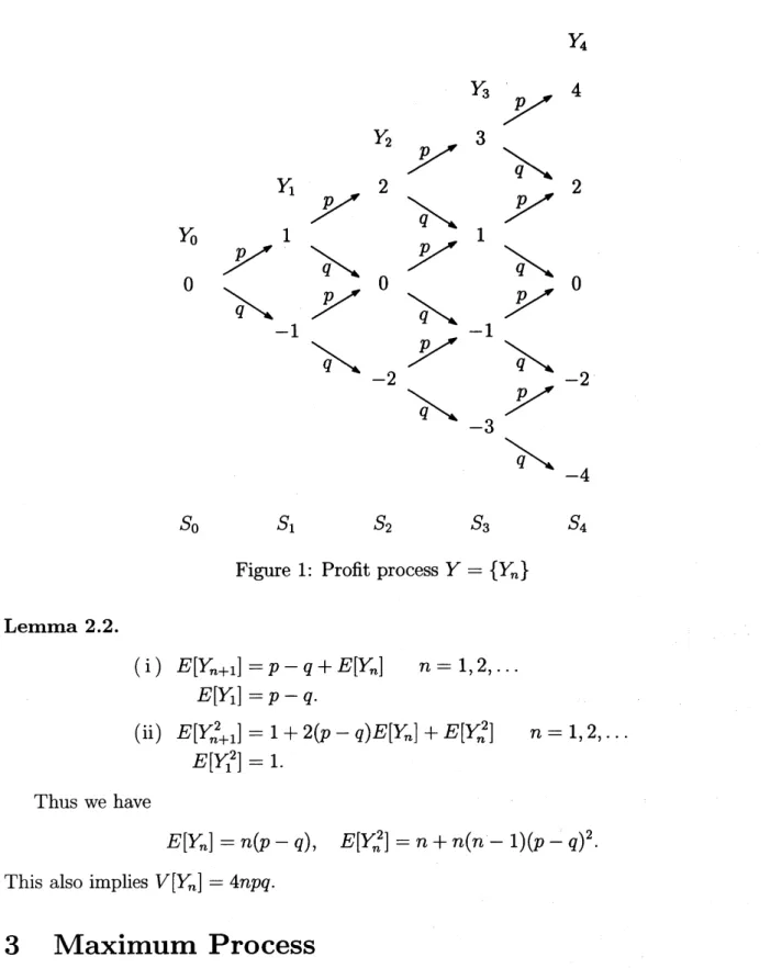
Therefore, the profit process $\{\mathrm{Y}_{n}, n=0,1, \ldots\}$ is aMarkov chain

on

the state spaces

$\{S_{n}\}$ with the transition probability _{$p=\{p_{n}(j|i)\}$} (Figure 1) :

$p_{n}(j|i)=\{$

$p$ if $j=i+1$

$q$ if

$j=i-1$

0otherwise

$n=0,1$, $\ldots$ . (3)

Then the recursion $\mathrm{Y}_{n+1}=X_{n+1}+\mathrm{Y}_{n}$, $n=1,2$, _$\ldots$ together with i.i.d. property in $\{X_{n}\}$

$\mathrm{Y}_{4}$ $\mathrm{Y}_{3}\nearrow^{p}$ 4 $\mathrm{Y}_{2}\nearrow p$ 3 $\backslash _{q}$ $\mathrm{Y}_{1}\nearrow p$ 2 $\backslash _{q}$ $\nearrow p$ 2 $\mathrm{Y}_{0}$ 1 1

$\nearrow p$ $\backslash _{q}$ $\nearrow^{p}$ $\backslash _{q}$

000

$\backslash _{q}$ $\nearrow^{p}$

$\backslash _{q}$ $\nearrow^{p}$

-1 -1

$\backslash _{q}$ $\nearrow p$ $\backslash _{q}$

-2 -2 $\backslash _{q}$ $\nearrow p$ -3 $\backslash _{q}$ -4 $S_{0}$ $S_{1}$ $S_{2}$ $S_{3}$ $S_{4}$

Figure 1: Profit process $\mathrm{Y}=\{\mathrm{Y}_{n}\}$ Lemma 2.2.

(i) $E[\mathrm{Y}_{n+1}]=p-q+E[\mathrm{Y}_{n}]$ $n=1,2$,$\ldots$

$E[\mathrm{Y}_{1}]=p-q$. (i) $E[\mathrm{Y}_{n+1}^{2}]=1+2(p-q)E[\mathrm{Y}_{n}]+E[\mathrm{Y}_{n}^{2}]$ $n=1,2$, $\ldots$ $E[\mathrm{Y}_{1}^{2}]=1$. Thus we have $E[\mathrm{Y}_{n}]=n(p-q)$, $E[\mathrm{Y}_{n}^{2}]=n+n(n-1)(p-q)^{2}$.

This also implies $V[\mathrm{Y}_{n}]=Anpq$.

3Maximum Process

It is shown that expected value and variance of profit $\mathrm{Y}_{n}$ has been calculated through

the Binomial distribution. In this section we consider expected value and variance of

maximum profit $Z_{n}$.

Lemma 3.1. (i) For$n=1,2$,$\ldots$,

$\mathrm{Y}_{2n+1}>Z_{2n}$

is equivalent to $X_{2}+X_{3}+X_{4}+X_{5}+\cdots+X_{2n-4}+X_{2n-3}+X_{2n-2}+X_{2n-1}\geq 0$ $X_{4}+X_{5}+\cdots+X_{2n-4}+X_{2n-3}+X_{2n-2}+X_{2n-1}\geq 0$ . $\cdot$ . $X_{2n-4}+X_{2n-3}+X_{2n-2}+X_{2n-1}\geq 0$ $X_{2n-2}+X_{2n-1}\geq 0$ $X_{2n}=X_{2n+1}=1$.

(ii) For$n=1,2$,$\ldots$ ,

$\mathrm{Y}_{2n+2}>Z_{2n+1}$ is equivalent to $X_{3}+X_{4}+X_{5}+X_{6}+\cdots+X_{2n-3}+X_{2n-2}+X_{2n-1}+X_{2n}\geq 0$ $X_{5}+X_{6}+\cdots+X_{2n-3}+X_{2n-2}+X_{2n-1}+X_{2n}\geq 0$ . $\cdot$ . (4) $X_{2n-3}+X_{2n-2}+X_{2n-1}+X_{2n}\geq 0$ $X_{2n-1}+X_{2n}\geq 0$ $X_{2n+1}=X_{2n+2}=1$. In particular, $\mathrm{Y}_{2}>Z_{1}$ is equivalent to $X_{2}=1$

.

(iii) In either case we have

$\mathrm{Y}_{n+1}-Z_{n}=1$ (5)

$\mathrm{Y}_{n+1}^{2}-Z_{n}^{2}=2\mathrm{Y}_{n}+1$ $n=0,1$,

$\ldots$ . (6)

$Pro\mathrm{o}/$

.

Since (i) is shown,

we

first show (ii). We note that the inequality

$\mathrm{Y}_{2n+2}>Z_{2n+1}$

$=\mathrm{Y}_{1}\vee \mathrm{Y}_{2}\vee\cdots\vee \mathrm{Y}_{2n-1}\vee \mathrm{Y}_{2n}\vee \mathrm{Y}_{2n+1}$

is equivalent to the system ofinequalities

$\mathrm{Y}_{2n+2}>\mathrm{Y}_{2n+1}$ $\Rightarrow X_{2n+2}>0$ $\mathrm{Y}_{2n+2}>\mathrm{Y}_{2n}$ $\Rightarrow X_{2n+2}+X_{2n+1}>0$ $\mathrm{Y}_{2n+2}>\mathrm{Y}_{2n-1}$ $\Rightarrow X_{2n+2}+X_{2n+1}+X_{2n}>0$ $\mathrm{Y}_{2n+2}>\mathrm{Y}_{2n-2}$ $\Rightarrow X_{2n+2}+X_{2n+1}+X_{2n}+X_{2n-1}>0$

.

$\cdot$

.

$\mathrm{Y}_{2n+2}>\mathrm{Y}_{2}$ $\Rightarrow X_{2n+2}+X_{2n+1}+\cdots+X_{3}>0$ $\mathrm{Y}_{2n+2}>\mathrm{Y}_{1}$ $\Rightarrow X_{2n+2}+X_{2n+1}+\cdots+X_{3}+X_{2}>0$.

$X_{2n+2}=1$ $X_{2n+1}=1$ $X_{2n}>-2$ $X_{2n-1}+X_{2n}>-2$ $X_{2n-2}+X_{2n-1}+X_{2n}>-2$ (7) . $\cdot$

.

$X_{3}+X_{4}+\cdots+X_{2n-1}+X_{2n}>-2$ $X_{2}+X_{3}+X_{4}+\cdots+X_{2n-1}+X_{2n}>-2$.

Since each $X_{m}$ takes only two values -1, 1,

we see

that (7) is equivalent to (4). (iii) is

shown as follows. First

we assume

that $\mathrm{Y}_{n+1}>Z_{n}$. Here

$\mathrm{Y}_{n}=\mathrm{Y}_{n-1}+X_{n}$

$>\mathrm{Y}_{n-1}$ (since _{$X_{n}=1$})

$\mathrm{Y}_{n}=\mathrm{Y}_{n-2}+X_{n-1}+X_{n}$

$\geq \mathrm{Y}_{n-2}$

$\mathrm{Y}_{n}=\mathrm{Y}_{n-3}+X_{n-2}+X_{n-1}+X_{n}$

$>\mathrm{Y}_{n-3}$ (since $X_{n-2}+X_{n-1}\geq 0$)

$\mathrm{Y}_{n}=\mathrm{Y}_{n-4}+X_{n-3}+X_{n-2}+X_{n-1}+X_{n}$

$\geq \mathrm{Y}_{n-4}$

.

$\cdot$

.

Then we have $Y_{n}\geq \mathrm{Y}_{m}$, $m=1,2$,

$\ldots$ ,$n$, which implies

$\mathrm{Y}_{n+1}-Z_{n}=\mathrm{Y}_{n+1}-\mathrm{Y}_{n}=X_{n+1}=1$.

Furthermore, this implies

$\mathrm{Y}_{n+1}^{2}-Z_{n}^{2}=(\mathrm{Y}_{n+1}+Z_{n})(Y_{n+1}-Z_{n})$

$=Y_{n+1}+Z_{n}$

$=2\mathrm{Y}_{n+1}-1$ $=2\mathrm{Y}_{n}+1$.

$\square$

Then we have the following recursion formulae :

Lemma 3.2.

(i) $E[Z_{n+1}]=P(\mathrm{Y}_{n+1}>Z_{n})+E[Z_{n}]$ $n=1,2$, $\ldots$ $E[Z_{1}]=p-q$_.

(ii) $E[Z_{n+1}^{2}]=E[(2\mathrm{Y}_{n}+1)\cdot 1_{\{\mathrm{Y}_{n+1}>Z_{n}\}}]+E[Z_{n}^{2}]$ $n=1,2$,

$\ldots$

$E[Z_{1}^{2}]=1$.

Proof.

First

we

note the equality

$1_{\{\mathrm{Y}_{n+1}>Z_{n}\}}+1_{\{\mathrm{Y}_{n+1}\leq Z_{n}\}}=1$

where $1_{A}$ is the characteristic function of set $A$ :

$1_{A}(\omega)=\{$ 1if $\omega$ $\in A$ 0otherwise. It holds that $Z_{n+1}=Z_{n}\vee \mathrm{Y}_{n+1}$ $=(Z_{n}\vee \mathrm{Y}_{n+1})\cdot(1_{\{\mathrm{Y}_{n+1}>Z_{n}\}}+1_{\{\mathrm{Y}_{n+1}\leq Z_{n}\}})$

$=\mathrm{Y}_{n+1}\cdot 1_{\{\mathrm{Y}_{n+1}>Z_{n}\}}+Z_{n}\cdot 1_{\{\mathrm{Y}_{n+1}\leq Z_{n}\}})$

$=(Y_{n+1}-Z_{n})\cdot 1_{\{\mathrm{Y}_{n+1}>Z_{n}\}}+Z_{n}$ (8)

$Z_{n+1}^{2}=(Z_{n}\vee \mathrm{Y}_{n+1})^{2}$

$=(Z_{n}\vee \mathrm{Y}_{n+1})^{2}\cdot(1_{\{\mathrm{Y}_{n+1}>Z_{n}\}}+1_{\{\mathrm{Y}_{n+1}\leq Z_{n}\}})$

$=\mathrm{Y}_{n+1}^{2}\cdot 1_{\{\mathrm{Y}_{n+1}>Z_{n}\}}+Z_{n}^{2}\cdot 1_{\{\mathrm{Y}_{n+1}\leq Z_{n}\}})$

$=(\mathrm{Y}_{n+1}^{2}-Z_{n}^{2})\cdot 1_{\{\mathrm{Y}_{n+1}>Z_{n}\}}+Z_{n}^{2}$. (9)

Prom (5)

we see

that

$E[(\mathrm{Y}_{n+1}-Z_{n})\cdot 1_{\{\mathrm{Y}_{n+1}>Z_{n}\}}]=E[1_{\{\mathrm{Y}_{n+1}>Z_{n}\}}]$

$=P(\mathrm{Y}_{n+1}>Z_{n})$.

Taking the expectation of both sides in (8),

we

have

$E[Z_{n+1}]=E[(\mathrm{Y}_{n+1}-Z_{n})\cdot 1_{\{\mathrm{Y}_{n+1}>Z_{n}\}}]+E[Z_{n}]$ $=P(\mathrm{Y}_{n+1}>Z_{n})+E[Z_{n}]$.

Similarly, acombination of (6) and (9) yields

$E[Z_{n+1}^{2}]=E[(\mathrm{Y}_{n+1}^{2}-Z_{n}^{2})\cdot 1_{\{\mathrm{Y}_{n+1}>Z_{\mathfrak{n}}\}}]+E[Z_{n}^{2}]$

$=E[(2\mathrm{Y}_{n}+1)\cdot 1_{\{\mathrm{Y}_{n+1}>Z_{n}\}}]+E[Z_{n}^{2}]$.

$\square$

4Markovization

The profit process $\{\mathrm{Y}_{n}, n\geq 0\}$ is aMarkov chain, where the state spaces _{$\{S_{n}\}$} and the

transition probability $p=\{p_{n}(j|i)\}$

are

defined by (2) and (3), respectively. Now we

consider the maximum profitprocess $\{Z_{n}, n\geq 1\}$, which is not necessarily Markov. We

are

interestedin

some

approachwhich makes the maximum process Markov

on

asuitable

state spaces. In the case, the statespaces

are

meaningful

as

far

as

it is small We call this

problemaMarkovization of process $\{Z_{n}\}$

.

In this section the Markovization is performed

through

an

invariant imbedding method [1, p.82], [13, Chap

.

Let us define the past-value sets $\{\Omega_{n}\}$

as

follows :

$\Omega_{n}:=\{\lambda_{n}|\lambda_{n}=(-1)\vee y_{1}\vee y_{2}\vee\cdots\vee y_{n-1}, y_{i}\in S_{i}, 1\leq i\leq n-1\}$

$n=2,3$,$\ldots$ .

In particular, we call $\Omega_{n}$ the maximum-value-set to date _$n$. Then the past-value sets

satisfy the forward recursive formula :

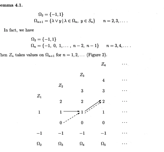
Lemma 4.1.

$\Omega_{2}=\{-1,1\}$

$\Omega_{n+1}=$

{A

$\vee y|\lambda\in\Omega_{n}$, $y\in S_{n}$

}

$n=2,3$, _$\ldots$ .

In fact, we have

$\Omega_{2}=\{-1,1\}$

$\Omega_{n}=\{-1,0,1, \ldots, n-2, n-1\}$ $n=3,4$,$\ldots$ .

Then $Z_{n}$ takesvalues

on

$\Omega_{n+1}$ for $n=1,2$,

$\ldots$ (Figure 2). $Z_{4}$ $Z_{3}$ $Z_{2}$ 33 $Z_{1}$ 22 3 1 1 \prime\prime\prime $1$

0\prime\prime\prime’

_{0 0} -1 -1 -1 -1

$\Omega_{2}$ $\Omega_{3}$ $\Omega_{4}$ $\Omega_{5}$

Figure 2: Maximum profit process $Z=\{Z_{n}\}_{n\geq 1}$

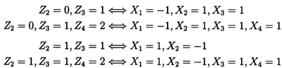
Lemma 4.2. However the maximum profit process $Z=\{Z_{n}, n\geq 1\}$ is not Markov on

the state spaces $\{\Omega_{n+1}\}$. Infact, both transition probabilities

$P(Z_{4}=2|Z_{2}=0, Z_{3}=1)=p$

and

$P(Z_{4}=2|Z_{2}=1, Z_{3}=1)=p^{2}$

depend on the yesterday’s state and are not equal

_for

$0<p<1$.

Proof.

The following four equivalences

axe

easily shown.

$Z_{2}=0$,$Z_{3}=1\Leftrightarrow X_{1}=-1$,$X_{2}=1$,$X_{3}=1$

$Z_{2}=0$,$Z_{3}=1$,$Z_{4}=2\Leftrightarrow X_{1}=-1$,_{$X_{2}=1,X_{3}=1$},$X_{4}=1$

$Z_{2}=1$,$Z_{3}=1\Leftrightarrow X_{1}=1$,_{$X_{2}=-1$}

$Z_{2}=1$,$Z_{3}=1$,$Z_{4}=2\Leftrightarrow X_{1}=1$,_{$X_{2}=-1$},_{$X_{3}=1$},_{$X_{4}=1$}.

The first two and the last two yield the former transition probability and the latter,

respectively. This completes the proof. $\square$

$(\mathrm{Y}_{4;}\lambda_{4})$ $\mathrm{Y}_{1}$ 1 $\mathrm{Y}_{0}$ 0 -1 (4; 3) (2; 3) (2; 2) (0; 2) (2; 1) (0; 1) (-2; 1) (0; 0) (-2; 0) (0;-1) (-2;-1) (-4;-1)

$\tilde{S}_{0}$ $\tilde{S}_{1}$ $\tilde{S}_{2}$ $\tilde{S}_{3}$ $\tilde{S}_{4}$

Figure 3: Expanded profit process $\tilde{\mathrm{Y}}=\{\tilde{\mathrm{Y}}_{n}, n\geq 0\}$

First, by attaching $\Omega_{n}$,

we

expand the state space $S_{n}$ to augmented state spaces $\{\tilde{S}_{n}\}$

as

foUows :

$\tilde{S}_{n}:=S_{n}$, $n=0,1$

$\tilde{S}_{n}:=\{(y_{n};\lambda_{n})|yi_{\dot{l}}^{=x_{1}+x_{2}+\cdots+x_{\dot{l}}}\lambda_{n}=y_{1}\vee y_{2}\vee\cdots\vee y_{n-1}\in\{-1,1\},1\leq i\leq n$ $\}\subset S_{n}\cross\Omega_{n}$ $n=2,3$,

$\ldots$ ,$N$.

Then the expanded state spaces $\{\tilde{S}_{n}\}$

are

forwardly generated

as

follows

Lemma 4.3.

$\tilde{S}_{2}=\{(2;1), (0;1), (0;-1), (-2;-1)\}$

$\tilde{S}_{n+1}=$

{

$(y+x$;A_{$\vee y$}) $|(y;\lambda)\in\tilde{S}_{n},$ _{$x\in\{-1,1\}$}

}

$n=2,3$,

$\ldots$ ,$N$.

Second we define

anew

transition law $q=\{q_{n}\}$ there by

$q_{0}(j|0):=\{$ $p$ if $j=1$ $q$ if $j=-1$ $q_{1}((j;i)|i):=\{$ $p$ if $j=i+1$ $q$ if

$j=i-1$

$q_{n}((j;\mu)|(i;\lambda)):=\{$

$p_{n}(j|i)$ if A$\vee i=\mu$

0otherwise $n=2,3$, $\ldots$ .

Finally we define asequence of random variables $\{\tilde{Y}_{n};n=0,1, \ldots\}$ by

$\tilde{\mathrm{Y}}_{n}:=\mathrm{Y}_{n}$ $n=0,1$; _{$\tilde{\mathrm{Y}}_{n}:=(Y_{n};\lambda_{n})$}

$n=2,3$, $\ldots$ .

We call $\tilde{Y}=\{\tilde{Y}_{n}\}$ an expanded profit process. Thus $Y_{n}$ represents today’s profit, which

behaves stochastically. And $\lambda_{n}=( 1)\vee y_{1}\vee y_{2}\vee\cdots\vee y_{n-1}=z_{n-1}$denotes the

mcvximum-tO-yesterday, which has beenalready determined. Thus $\{\lambda_{n}\}$ is deterministic. Everytime

$Y_{n}$ realizes avalue $y_{n}$, the resulting pair $(y_{n};\lambda_{n})$ yields the today’s maximum-value

$\lambda_{n}\vee y_{n}=y_{1}\vee\cdots\vee y_{n-1}\vee y_{n}=z_{n}$

under maximum operation V. In other words, the expanded profit process $\tilde{\mathrm{Y}}=\{\tilde{\mathrm{Y}}_{n}\}$

generates the maximum process $Z=\{Z_{n}\}$ under the binary operation. Furthermore, we

have the following desired property.

Lemma 4.4. The expanded profit process $\{\tilde{\mathrm{Y}}_{n}, n\geq 0\}$ is a Markov chain on the state

spaces $\{\tilde{S}_{n}\}$ $with$ the transition probability _{$q=\{q_{n}\}$} (Figure 3).

We define amapping $T_{n}$ : $\tilde{S}_{n}arrow R^{1}$ by

$T_{n}(\tilde{y}_{n}):=\lambda_{n}\vee y_{n}$ $n=2,3$,

–

Then the sequence ofmappings $\{T_{n}\}$ transforms process $\{\tilde{\mathrm{Y}}_{n}\}$ into _{$\{Z_{n}\}$} in the following

sense :

$T_{n}(\tilde{Y}_{n})=Z_{n-1}\vee Y_{n}=Z_{n}$ $n=2,3$,

$\ldots$ .

Thustheprocess $\{\tilde{\mathrm{Y}}_{n}\}$ is aMarkovization of_{$\{Z_{n}\}$}. Thus the Markovization is astochastic

version ofthe final state model [1, p.82], [13, p.71]

4.1

Recursion for

$E[Z_{N}]$

Now let

us

take apositiveinteger $N(\geq 2)$. We derive arecursive formula for the expected

value of the maximum random variable$Z_{N}$. We define

a

$te$ minal

function

$T:\tilde{S}_{N}arrow R^{1}$

by

$T(\tilde{y}_{N}):=\lambda_{N}\vee y_{N}$.

Lemma 4.5. $Jt$ holds that

$E[Z_{N}]=\tilde{E}_{\tilde{y}0}[T(\tilde{\mathrm{Y}}_{N})]$

where $\tilde{E}_{\tilde{y}0}$ is the expectation operator induced

from

the transition law $q$ and the initial

state $\tilde{y}_{0}=y_{0}=0$.

Let

us

define the sequence ofexpected value functions $\{u_{n}\}$

as

follows :

$u_{n}(\tilde{y}_{n}):=\tilde{E}_{\tilde{y}_{n}}[T(\tilde{Y}_{N})]$ $n=0,1$,

$\ldots$ ,$N-1$

$u_{N}(\tilde{y}_{N}):=\lambda_{N}\vee y_{N}$

where$\tilde{E}_{\tilde{y}_{n}}$ is theexpectationoperator induced from thetransition law $\{q_{n}, q_{n+1}, \ldots, q_{N}\}$

and

an

initial state $\tilde{y}_{n}\in\tilde{S}_{n}$

.

We remark that $\tilde{y}_{n}$ takes the following values :

$\tilde{y}_{0}=y_{0}=0$, $\tilde{y}_{1}=y_{1}=-1$

or

1, $y\sim n=(y_{n};\lambda_{n})$ $n=2,3$,

$\ldots$ ,$N$.

Then

we

have the backward recursive formula :

Theorem 4.1.

$u_{0}(0)= \sum_{j\in S_{1}}u_{1}(j)q_{0}(j|0)$

$u_{1}(i)= \sum_{j\in S_{2}}u_{2}(j;i)q_{1}(j|i)$ $i\in S_{1}$

$u_{n}(i; \lambda)=\sum_{j\in S_{n+1}}u_{n+1}$(

$j$;A$\vee i$)_{$q_{n}(j|i)$} $(i;\lambda)\in\tilde{S}_{n}$, $n=2,3$,

$\ldots$ ,$N-1$ (10)

$u_{N}(i;\lambda)=\lambda\vee i$ $(i;\lambda)\in\tilde{S}_{N}$.

Thus, successively solving (10),

we

have the desired expected value of the maximum

profit $Z_{N}$

over

$N$-stage problem :

$u_{0}(0)=E[Z_{N}]$

.

Actually the recursive formula reduces

as

follows :

Corollary 4.1.

$u_{0}(0)=pu_{1}(1)+qu_{1}(-1)$

$u_{1}(i)=pu_{2}(i+1;i)+qu_{2}(i-1;i)$ $i=-1,1$ $u_{n}(i;\lambda)=pu_{n+1}$($i+1$;A$\vee i$) _{$+qu_{n+1}(i-1;\lambda\vee i)$}

$(i;\lambda)\in\tilde{S}_{n}$, $n=2,3$,

$\ldots$ ,$N-1$

$u_{N}(i;\lambda)=\lambda\vee i$ $(i;\lambda)\in\tilde{S}_{N}$.

4.2

Recursion for

$E[Z_{N}^{2}]$

Now let us consider the expectedvalue of the squared random variable$Z_{N}^{2}$

.

Here in place

of the terminal function $T$

we

introduce the squared terminal

function

$T^{2}$ : $\tilde{S}_{N}arrow R^{1}$ by

$T^{2}(\tilde{y}_{N}):=(\lambda_{N}\vee y_{N})^{2}$.

Then we have

Lemma 4.6. It holds that

$E[Z_{N}^{2}]=\tilde{E}_{\tilde{y}0}[T^{2}(\tilde{\mathrm{Y}}_{N})]$.

Let us define $\{v_{n}\}$

as

follows :

$v_{n}(\tilde{y}_{n}):=\tilde{E}_{\tilde{y}_{n}}[T^{2}(\tilde{\mathrm{Y}}_{N})]$ $n=0,1$, $\ldots$ ,$N-1$ $v_{N}(\tilde{y}_{N}):=(\lambda_{N}\vee y_{N})^{2}$. Then we have Theorem 4.2. $v_{0}(0)=pv_{1}(1)+qv_{1}(-1)$ $v_{1}(i)=pv_{2}(i+1;i)+qv_{2}(i-1;i)$ $i=-1,1$

$v_{n}(i;\lambda)=pv_{n+1}$($i+1$;A$\vee i$) _{$+qv_{n+1}$}($i-1$;A$\vee i$) (11)

$(i;\lambda)\in\tilde{S}_{n}$, $n=2,3$,

$\ldots$ ,$N-1$

$v_{N}(i;\lambda)=(\lambda\vee i)^{2}$ $(i;\lambda)\in\tilde{S}_{N}$.

Thus, the recursive computation of (11) yields the desired expected value:

$v_{0}(0)=E[Z_{N}^{2}]$.

4.3

Recursion

for

$P(Z_{N}=k)$

Now let us consider the probability distribution of $Z_{N}$. For each fixed $k\in\Omega_{n\dagger 1}$ the

probability it takes value $k$ is calculated through invariant imbedding. We define the

terminal function $T:\tilde{S}_{N}arrow R^{1}$ by

$T(\tilde{y}_{N}):=\psi(\lambda_{N}\vee y_{N})$

where $\psi(\cdot)$ is the indicator function ofaone-point set _$\{k\}$ :

$\psi(z):=1_{\{k\}}(z):=\{$ 1if $z=k$

0otherwise Then

Lemma 4.7. It holds that

$P(Z_{N}=k)=\tilde{E}_{\tilde{y}0}[T(\tilde{Y}_{N})]$.

Further we define $\{w_{n}\}$

as

follows : $w_{n}(\tilde{y}_{n}):=\tilde{E}_{\tilde{y}_{n}}[T(\tilde{Y}_{N})]$ $n=0,1$, $\ldots$ , $N-1$ $w_{N}(\tilde{y}_{N}):=\psi(\lambda_{N}\vee y_{N})$. Then Theorem 4.3. $w_{0}(0)=pw_{1}(1)+qw_{1}(-1)$ $1;\mathrm{i})=pw_{2}(i+1;i)+qw_{2}(i-1;i)$ $i=-1,1$

$Wn(i;\lambda)=pw_{n+1}$($i+1$;A$\vee i$)_{$+qw_{n+1}$}($i-1$;A$\vee i$) (12)

$(i;\lambda)\in\tilde{S}_{n}$, $n=2,3$,

$\ldots$ ,$N-1$

$w_{N}(i;\lambda)=\psi(\lambda\vee i)$ $(i;\lambda)\in\tilde{S}_{N}$.

Thus, the recursion (12) yields the desired probability :

$w_{0}(0)=P(Z_{N}=k)$

.

References

[1] R.E. Belman, Dynamic Programming, Princeton Univ. Press, NJ, 1957.

[2] R.E. Bellman, Some Vistas

_of

Moderm Mathematics, University ofKentucky Press,

Lexington, KY,

1968.

[3] List of Publications :Richard Bellman, IEEE Transactions

on

Automatic Control,

AC-26(1981), No. $5(\mathrm{O}\mathrm{c}\mathrm{t}.)$,

1213-1223.

[4] R.E. Bellman, Eye

_of

the Hurricane

:an

Autobiography, WorldScientific, Singapore,

1984.

[5] R.E. Bellman(Ed. R.S. Roth), The Bellman Continuum :A Collection

_of

the Works

of

Richard Bellman, World Scientific, Singapore, 1986.

[6] R.E. Bellman and E.D. Denman, Invariant Imbedding, Lect. Notes in Operation

Research and Mathematical Systems, Vol. 52, Springer-Verlag, Berlin, 1971.

[7] R.E. Bellman and E.D. Denman, Invariant Imbedding :Proceedings

_of

the Summer

Workshop

on

Invariant Imbedding Held at the University

_of

Southerm California,

June -August 1970, Lect. Notes in Operation Research and Mathematical Systems,

Vol. 52, Springer-Verlag, Berlin, 1971.

[8] S. Iwamoto, Theory

_of

Dynamic Program :Japanese, KyushuUniv. Press, Fukuoka,

1987.

[9] S. Iwamoto, Maximizing threshold probability through invariant imbedding, Eds.

HF. Wang and U.P. Wen, Proceedings

_of

The Eighth BELLMAN CONTINUUM,

Hsinchu, ROC, Dec.2000, pp.17-22

[10] S. Iwamoto, Fuzzy decision-making through three dynamic programming

proaches, Eds. H.F. Wang and U.P. Wen, Proceedings

_of

The Eighth $BEL\ovalbox{\tt\small REJECT}$

CONTINUUM, Hsinchu, ROC, Dec.2000, pp.23-27.

[11] E.S. Lee, Quasilinearization and Invariant Imbedding, Academic Press, New $\urcorner$

1968.

[12] S. Ross, Stochastic Processes :second edition, Wiley&Sons, New York, 1996.

[13] M. Sniedovich, Dynamic Programming, Marcel Dekker, Inc. NY, 1992