Abstract. This report is also about an example of the stabilization techniques developed by Shi-rayanagi and Sweedler.
We previously used bracket coefficients to make an experiment ofcomputing floating point Gr\"obner bases. A bracket coefficient is like a circular interval from interval analysis which indicates a center and
a rad$\mathrm{i}\mathrm{u}\mathrm{s}$. Another experiment to make would be using rectangular intervals indicating lower and upper
bounds, which also playan important role in numerical approximation. We used Maple’s package written by Connell and Corless for performing rectangular interval arithmetic in coefficients, in the course of Buchberger’s algorithm, where we judge a rectangular interval as zero if it contains zero. We obtained niceconvergence, stability and speed as well as the bracket coefficient version.
5.1
Introduction
多項式環における計算において、その基礎体が有理数の場合はしばしば係数膨張のため、多くの計算時間とス ペースがかかる。無理数を含むときはなおさら顕著である。よって、実際の計算においてはこれらの困難を解決し なくてはならない。昨年、 白柳 ([4]) はBuchberger’s algorithm ([2]) に対して、二つの浮動小数を $[A, \alpha]$ のよう
に組み合わせ、$A$ を中心とする半径 $\alpha$ の中に真の値が含まれるようにして計算を行なうcircular interval を用い
て近似算法を提案した。今回は rectangular interval を用いてそれを実装し、浮動小数点近似 Gr\"obnerbasis の計算を行なった。
5.2
Interval
Arithmetic
rectangular interval は$[a_{1}, a_{2}]$ ($a_{1},$ $a_{2}$は浮動小数) で、$\{x|a_{1}\leq x\leq a_{2}\}$ を表すものである。演算は以下
の通りである $([1])_{0}$
.加法
$[a_{1}, a_{2}]+[b_{1}, b_{2}]=[a_{1}+b_{1}, a_{2}+b_{2}]$
. 減法
$[a_{1}, a_{2}]-[b_{1}, b_{2}]=[a_{1}-b_{2}, a_{2}-b_{1}]$
.乗法
$[a_{1}, a_{2}] \cross[b_{1}, b_{2}]=[\min(a_{1}b_{1}, a_{1}b_{2}, a2b_{1}, a_{2}b_{2}), \max(a_{1}b_{1}, a_{1}b2, a2b_{1}, a2b_{2})]$
実際の計算においては Maple VRelease 3([3]) の Share Library にある区間演算パッケージ intpak (by Connell, A.
&Corless,
R. M) を用いた。(ただし区間の下限では切捨て、上限では切上げによる浮動小数演算を行なっている。) 多項式の係数問の計算にはこの intpak を用い、多項式の変数とのインタ$-$フェイス $(([a_{1}, a_{2}]X+$
$[b_{1}, b_{2}]y)2$など) は尾崎が作成した。
5.3
Zero Judgement
&Supportwise
Con-vergence
Buchberger’s algorithm において、係数を区間にして計算を行なうときの問題は、 どういう区間を “零” と
みなすかである。[4] の提案する circular interval に対する判定法は、
$[A, \alpha]$が “零” $\Leftrightarrow \mathrm{d}\mathrm{c}\mathrm{f}|A|\leq\alpha$
であった。 これに対応して rectangular 版は、
$[a, b]$が“零” $\Leftrightarrow 0\mathrm{d}\mathrm{c}\mathrm{f}\in[a, b]$
となる。
この判定法を使うことによって、次のように Supportwise Convergence という収束性が得られる。
定理 531. 精度 $\mu$ での区間演算を使い、 上の判定法に従った Buchberger’s algorithm の出力を
$G^{\mu}$ とする。
また、exact な計算における出力 (真のグレブナ基底) を $G$ とする。その時$G^{\mu}$は$G$ に係数ごとに収束し、かつ、
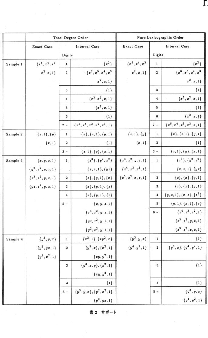
ここに、多項式 $f= \sum$ 。 $a_{\alpha}x^{\alpha}$ に対し $\{x^{\beta}|a\rho\neq 0\}$ を多項式のサポートという。多項式の集合のサポー トは、各元のサポ– }$\mathrm{c}$ の集合である。定理の証明は [4] を参照されたい。circular版における議論と並行な議論が rectangular版においても成り立つ。
5.4
Results
前述の Maple V Release 3の intpak を用いて浮動小数係数の Buchberger’s algorithm を実装し、$\mathrm{S}\mathrm{u}\mathrm{p}-$
portwise Convegence を観測した。計算機は $\mathrm{H}\mathrm{P}9000/735$ である。項順序としては、Total Degree Reverse
Lexicographic Order と Pure Lexicographic Order を用いた。なお、これらの順序は Maple の内部関数とし て実装されている。各変数の順序は
$x>y>z$
とし、浮動小数点の精度は $1\sim 10$ までの範囲で行なった。出力 結果に関しては最後を参照されたい。 サンプルは以下の多項式の集合で生成されるイデアルを用いた。 Sample 1 $[(x^{2}- \frac{1}{9})^{5},$ $(x^{2}+ \frac{2}{3}x+\frac{1}{9})^{5}]$ Sample 2$[y-z+1,$$\frac{2}{3}x+\frac{1}{3}y-z+\frac{5}{3},$
$-x+y+z-2]$
Sample 3
$[$ $\frac{1}{7}x^{2}-\frac{3265483908\mathrm{s}46\mathrm{s}2}{27297401\tau 239}x+\frac{1263781236281}{7126s\S 126}y^{2}+\frac{268726\tau 2361\epsilon 27}{7263188218281}z^{2}$, $\frac{3}{8}xy+\frac{123\epsilon 78126s8123}{763812368213132}yz-\frac{63812638126}{77263812831}y$,
$\frac{4}{9}x+\frac{3270912709\gamma 9304}{2412237\mathrm{s}460421}y+\frac{18467031\mathrm{s}9\mathrm{s}309203}{3184054\mathrm{s}9032}Z-\frac{356318063693141319}{6436561806418109}$ $]$
Sample 4
$[ \sqrt{2}ex^{3}y+\sqrt{3}xy+\frac{\sqrt{7}}{e},$$\frac{\sqrt{3}}{e}x^{2}y^{2}-\sqrt{7}xy+\frac{e}{\sqrt{11}}]$
Sample 5
$[ \frac{\sqrt{2}e}{\pi}x^{3}y+(\sqrt{3}+\pi)xy+\frac{\sqrt{7}}{(e-\pi)},$ $\frac{(1-e\sqrt{3})}{e}\pi x^{2}y^{2}-(\sqrt{7}-e)xy+\frac{e}{\sqrt{11}}]$
表1に計算時間を示す。計算時間は浮動小数点の精度が $5\sim 10$ までを挙げてある。 これらは各20回忌つ行ない
5.5 Conclusion
この計算結果から計算時間に関しては、与えられた多項式が簡単な場合には浮動小数点の計算をし
ているため逆に時間がかかってしまうが、係数が有理数であっても複雑であったり、無理数を含んでい る場合には計算時間を減らすことに成功している。 また計算結果について見てみると、 これらのサンプルの場合、精度が
5
を越えるとサポートが
–
致している。問題は収束する速度であるが、
これらの サンプルにおいては、-
桁の精度で収束することが確認された。今後の課題は、収束の速度やサポー トが正しいかどうかを判定する方法についての理論的な研究である。 追記:
講演のときに、サンプルが小さすぎるとの批判を頂いた。しかし、Sample 4 と Sample5 か らわかるように、正確演算では、係数を少し複雑にするだけで係数膨張の度合が格段に増大する。係数を Sample 5より更に複雑にしたら、$\mathrm{D}\mathrm{e}\mathrm{c}\mathrm{A}\mathrm{l}.\mathrm{p}\mathrm{h}\mathrm{a}$ 上の $\mathrm{R}\mathrm{i}\mathrm{s}\mathrm{a}/\mathrm{A}\mathrm{s}\mathrm{i}\mathrm{r}$ (富士通) でも、耐えられる時間
内に計算できなかった。一見小さく見える Sample 5 でさえ、係数膨張を攻略する 「我々の立場」で
は十分 “大きな” 例といえると思う。(浮動小数近似という立場からみれば係数の変化はあまり関係な
い。実際、Maple でさえ数秒で計算する。) とはいえ、我々のアプローチが真に有効であると主張す
るためには、更に多くの
“
大きな”
実例で示す必要があることに異論の余地はない。参考文献
$[1]\mathrm{A}\mathrm{l}\mathrm{f}\mathrm{e}\mathrm{l}\mathrm{d}$,
G.
andHerzberger,
J., Introduction toInterval
ComputationsComputer
Science
andApplied Mathematics Academic Press (1983)
$[2]\mathrm{B}\mathrm{u}\mathrm{c}\mathrm{h}\mathrm{b}\mathrm{e}\mathrm{r}\mathrm{g}\mathrm{e}\mathrm{r}$, B., Gr\"obner Bases: An
Algorithmic Method in
PolynomialIdeal
TheoryMulti-dimensional Systems
Theory (ed. Bose,N.
K.)184-232
D.
Reidel Publishing Company
(1985)$[3]\mathrm{C}\mathrm{h}\mathrm{a}x$,
B.
W., Geddes,K. O.,
Gonnet,G.
H.,Leeong, B.
L.,Monagan, M.
B., Watt,S.
M.,First Leaves: A
Tutorial
Introduction
toMaple V
Springer-Verlag
(1992)$[4]\mathrm{s}\mathrm{h}\mathrm{i}\mathrm{r}\mathrm{a}\mathrm{y}\mathrm{a}\mathrm{n}\mathrm{a}\mathrm{g}\mathrm{i}$, K.,
An
Algorithm
toCompute Floating Point
Gr\"obner Bases,Mathematical
5.7
Appendix: Output
計算出力を以下に挙げる。exact
な場合の出力は繁雑となり区間演算と比較しにくいので出力を浮
動小数点表示に直してある。フォ$-$マットは左から精度、時間、出力、zero judgement の回数である。
Sample