Analysis of In-Plane Problems for an Isotropic Elastic Medium with Many Circular Holes or Rigid Inclusions

and Materials

Engineering

Analysis of In-Plane Problems

for an Isotropic Elastic Medium with

Many Circular Holes or Rigid Inclusions

∗

Mutsumi MIYAGAWA

, Jyo SHIMURA

, Takuo SUZUKI

and

Takanobu TAMIYA

∗∗_{Dept.of Creative Manufacturing Tokyo Metropolitan College of Industrial Technology. Arakawa Campus}

8-17-1, Minami-senju, Arakawa-ku, Tokyo 116-0003, Japan E-mail: [email protected]

∗∗∗_{Tokyo National College of Technology}

1220-2, Kunugida-machi, Hachioji-shi, Tokyo 193-0997, Japan

Abstract

Key words : Isotropic Elasticity, In-Plane Problem, Many Cylindrical Holes, Many

Rigid Inclusions, Uniform Stress Loading

1. Introduction

A number of studies have examined the problems associated with disturbances around a single hole or rigid circular inclusion under in-plane loading, such as loading due to uniform stresses or a concentrated force at an arbitrary point. Therefore, these problems have many applications in engineering fields. These inclusion problems have proved to be very useful for mechanical analysis.

These problems have been developed further in order to observe the interacting distur-bances for multiple circular holes. However, these techniques have been applied using dif-ferent numerical analysis methods such as the finite element method (FEM) or the boundary element method (BEM). So, for example, if one engineer is an expert in FEM analysis of a model, while another engineer is not, their results will not be the same.

The purpose of the present study is to apply the reflection principle of Moriguchi(1)_, who investigated a single hole in in-plane problems, and the techniques of Honein(2)and Hi-rashima(4)∼(6)to consider anti-plane multi-hole problems. We obtained general solutions(7)(8) for up to two circular inclusions. Using these techniques, we expanded these problems to cases involving many circular holes or rigid inclusions.

In the present study, these holes or rigid inclusions have arbitrary arrangements and sizes inside the matrix. Using this explicit general solution, we present several numerical examples under uniform stresses at infinity.

2. Fundamental Equation and General Solution

In this section, we review the fundamental formulation of in-plane elastostatics and

Copyright © 2013 by JSME

*Received 4 July, 2013 (No. T2-10-0534) Japanese Original : Trans. Jpn. Soc. Mech.

Eng., Vol. 77, No. 774, A (2011), pp.251-260 (Received 12 July., 2010) [DOI: 10.1299/jmmp.7.540]

In this paper, we derive the general solutions for many cylindrical holes or rigid inclusions perfectly bonded to an elastic medium (matrix) of infinite extent, under In-Plane deformation. These many holes or rigid inclusions have different radii and different central points. The matrix is subjected to arbitrary loading like uniform stresses at infinity. The solution is obtained, via iterations of Möbius transformation as a series with an explicit general term involving the complex potential functions of the corresponding homogeneous problem. This procedure has been termed” heterogenization”. Using these solutions, several numerical examples are shown by graphical representation.

present the notation used herein. We consider the complex region z= x + iy, where i is the imaginary unit (i= √−1), to be infinite. Under in-plane deformations, there exist displace-ments ux and uy and stresses σx, σy, and τxy, which are obtained in Cartesian coordinates only.

The formulation used to find the stresses and displacements is satisfied by the complex potential functionsφ(z) and ψ(z), which are also used in the techniques of Moriguchi(1)_.

ux− iuy= 1 2GM [ κMφ(z) − { zφ′(z)+ ψ′(z)}]. (1) −Py− iPx= φ(z) + { zφ′(z)+ ψ′(z)}. (2)

where a prime indicates differentiation with respect to the complex variables z and κM as follows: κM= { (3− νM)/(1 + νM) Plane Stress 3− 4νM Plane Strain (3)

where GMandνMare the shear modulus and Poisson’s ratio for the matrix, respectively. Px and P_yindicate the resultant forces that act from right to left along an arbitrary course from point A to point B in the matrix.

Px= ∫B A ( σxdy − τxydx ) , P_y= ∫B A ( τxydy − σydx ) . (4)

Hence, the stresses are obtained as follows:

σx= 2Re[φ′(z)]− Re[zφ′′(z)+ ψ′′(z)], σy= 2Re[φ′(z)]+ Re[zφ′′(z)+ ψ′′(z)], τxy= Im [ zφ′′(z)+ ψ′′(z)],    (5)

where Re[ ] and Im[ ] are the real and imaginary parts, respectively, of the complex func-tion in parentheses, and the overbar indicates complex conjugafunc-tion.

2.2. General solution in the presence of a single circular hole

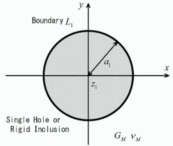
We first investigate the problem in the presence of a single circular hole or a rigid inclu-sion disturbing the uniform stressesσ∞_x,σ∞_y, andτ∞_xyat infinity. If the circular boundary is a hole, then the boundary is referred to as a free boundary, and if the circular boundary is a rigid inclusion, then the boundary is referred to as a fixed boundary. We consider the heterogeneous problem of the jthelastic circular inclusion perfectly bonded to an elastic matrix of infinite ex-tent. This matrix is given by the complex potential functionsϕ(z) and ψ(z). The matrix and the boundary produce an in-plane deformation, as shown in Fig. 1. We set the general boundary conditions of the tractions and displacements on the boundary Lj

(

i.e., z = zj+ ajeiθ )

between the jth _{hole and the matrix, where a}

jand zj(= (0, 0)) are the radius and origin, respectively, of the jth_{hole. In this subsection, we use j= 1 because there is only one inclusion.}

Required continuity of the tractions and displacements along the circular interface. Hole (Free boundary):

P( j)x = 0, P

( j)

y = 0. (6)

Rigid inclusion (Fixed boundary):

u( j)x = 0, u

( j)

y = 0. (7)

After subsection 2.4, it is not difficult to imagine that the center point of each hole will be moved by the interacting disturbances for many holes under the in-plane loading. These rigid movements of the holes or the inclusions would need a new supposition other than the boundary conditions defined in Eqs. (6) and (7). So, we consider that such rigid movements do not happen in this paper.

Fig. 1 Geometry of an infinite elastic medium with a single hole or rigid inclusion.

The most general complexes for this problem may be written as follows:

φM(z)= φ(z) + ˆf(z). (8)

χM(z)= χm(z)+ ˆg(z). (9)

Based on Eqs. (1) and (2), we setχ(z) as an auxiliary function in the following.

χM(z)= zφ′(z)+ ψ′(z) (10)

The matrix is an isotropic material and the central point of the circular boundary is the origin and its radius is a1. Using the mirror projection of a point z that was described by Moriguchi(1) on the boundary, we have a2

1/z. Hence, the auxiliary function χm(z) may be replaced by χm(z)=

a2₁

z φ

′_{(z)+ ψ}′_{(z), (11)}

where, f and g are arbitrary functions, after we establish ˆf(z) and ˆg(z) in the following

equation using the principle of mirror projection: ˆ f (z)= f(a2 1/z ) , g(z) = gˆ (a2 1/z ) . (12)

Equation (12) is obtained when the center of the jth hole coincides with the origin. This problem reduces to finding f andg such that the continuities given by Eqs. (1) and (2) are satisfied. Imposition of the boundary conditions Eqs. (6) and (7) yields

f (z)= 1

KMχ

m(z), g(z) = KMφ(z). (13)

Hence, we obtain the general solutions in this subsection in the following forms:

φM(z)= φ(z) + 1 KMχ m(a2₁/z), (14) χM(z)= χm(z)+ KMφ(a2₁/z). (15) where KM= { −1 Hole κM Rigid Inclusion (16)

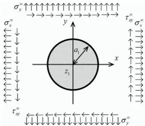
Fig. 2 Infinite elastic medium with a single hole or rigid inclusion under uniform stresses.

2.3. Problem in the presence of a single circular hole under uniform shear stresses In this section, we consider the problem of disturbing the uniform stressesσ∞_x,σ∞_y, and

τ∞

xyat infinity in Fig. 2. The fundamental complex potential functionsϕ(z), ψ′(z) are given at infinity|z| = ∞ as φ(z) = τ∗_{z, ψ}′_{(z)= 2τ}∗∗_{z, (17)} where τ∗₌ σ∞x + σ∞y 4 , τ ∗∗₌ σ∞y − σ∞x 4 + i τ∞ xy 2 . (18)

These functions do not have a singularity inside the region a1 < |z| < ∞. We consider the functions obtained by substituting Eq. (17) into Eqs. (14) and (15), and coinciding with the initial conditionσ∞_x,σ∞_y, andτ∞_xyat infinity. The auxiliary functionχ(z) defined in Eq. (11) at infinity|z| = ∞ reduces to

χm(z)≈ 2τ∗∗z. (19)

The functions obtained by substituting Eq. (19) into Eqs. (14) and (15) are general solutions in this subsection, and we obtain the following:

φM(z)= τ∗z+ 2τ∗∗ KM a2₁ z , (20) χM(z)= 2τ∗∗z+ KMτ∗ a2 1 z . (21)

These solutions coincide with the solution of Moriguchi(1) _{and Hirashima}(4)(5)_{. When the} central point of the boundary L1moves to the arbitrary point z1, Eqs. (20),(21) can be reduced to φM(z)= φ(z) + 1 KM χm   a2 1 z− z1 + z1  . (22) χM(z)= χm(z)+ KMφ   a2 1 z− z1 + z1  . (23)

Fig. 3 Geometry of an infinite elastic medium with many holes or rigid inclusions.

2.4. General solution in the presence of many circular holes

In this section, we use the solution presented in the previous section as a starting point for obtaining the solution of many circular holes that have radii ajand origins zj( j= 1, 2, · · · , Q), as shown in Fig. 3. In order to analyze the problem of rigid inclusions, we need only change the coefficient KMfrom−1 (Hole) to κM(Rigid inclusion).

This matrix is given by the complex potential functionsϕ(z) and ψ(z). We set the general boundary conditions, given by Eqs. (6) and (7), of the tractions and displacements. The proposed method can be regarded as an extension of the Schwarz alternating method, which, in principle, permits a solution to be obtained to any desired degree of accuracy. However, in the present study, the analysis is carried a step further. By exploiting the M¨obius transformation, the general term of the series is obtained, and thus the general solution is written as a rapidly convergent series with an explicit general term. To this end, we define

Ajz=

a2_j z− zj

+ zj, ( j = 1, 2, · · · , Q). (24)

Moreover, Aj specifies the operator with respect to the complex variable z. Normally, the left-hand side of Eq. (24) would be written as Aj(z). However, for convergence, in the present paper, we denote Ajz as in Eq. (24). Thus, AiAjz, for example, is expressed as follows:

AiAjz= Ai [ Aj(z) ] = a 2 i Aj(z)− zi + zi= a2_i    a 2 j z− zj + zj    − zi + zi. (25)

For the purpose of the multi-hole problem, we first considered the problem with three holes (i.e. Q= 3 ) as a simple case. After that, we produced the general solution for many holes (Q is arbitrary number). Using the same technique, we could satisfy the continuities given by Eqs. (1) and (2) for the boundary Lj. We first set ˆf1(z) and ˆg1(z) on L1as follows:

φM(z)= φ(z) + ˆf1(z). (26)

χM(z)= χm(z)+ ˆg1(z). (27)

These functions reduce to finding f1andg1such that the continuities on L1are satisfied. The following are obtained using sets ˆf2(z) and ˆg2(z) on L2:

φM(z)= φ(z) + 1

KM

χM(z)= χm(z)+ KMφ(A1z)+ ˆg2(z). (29)

These functions reduce to finding f2andg2such that the continuities on L2are satisfied. The following are obtained using sets ˆf3(z) and ˆg3(z) on L3:

φM(z)= φ(z) + 1 KMχ m(A1z)+ 1 KMχ m(A2z)+ φ(A1A2z)+ ˆf3(z). (30) χM(z)= χm(z)+ KMφ(A1z)+ KMφ(A2z)+ χm(A1A2z)+ ˆg3(z). (31)

Applying the continuity on L3, we obtain ˆf3(z) and ˆg3(z). Note that the boundary condition on

L1 is not satisfied for L2and L3by the previous steps. For this reason, we may set ˆf4(z) and ˆ

g4(z) to satisfy the continuity on L1.

φM(z)= φ(z) + 1 KMχ m(A1z)+ 1 KMχ m(A2z)+ φ(A1A2z)+ 1 KMχ m(A3z) + φ(A1A3z)+ φ(A2A3z)+ 1 KM χm(A1A2A3z)+ ˆf4(z). (32)

χM(z)= χm(z)+ KMφ(A1z)+ KMφ(A2z)+ χm(A1A2z)+ KMφ(A3z)

+ + χm(A1A3z)+ χm(A2A3z)+ KMφ(A1A2A3z)+ ˆg4(z). (33)

We applied the continuity on L1, repeating the previous steps and obtaining these additional terms each time. In this way, we could obtain the following explicit solution of the in-plane problem in the presence of many circular holes or rigid inclusions. To this end, we used

φM(z)= φ(z) + +∞_∑ n=1 φ(Mp(n)_q(n)z)+ 1 KM +∞_∑ n=0 χm(Aq(0)M_p(n)_q(n)z). (34) χM(z)= χm(z)+ +∞_∑ n=1 χm(Mp(n)_q(n)z)+ K_M +∞ ∑ n=0 φ(Aq(0)M_p(n)_q(n)z). (35)

The coefficients in the above expressions are given as follows. The arguments p(i), q(i)indicate different arguments from the index i and p(i), q(i)have values from 1 to Q. In addition, δp_q(i)(i)is Kronecker delta. Now, the right side functions of Eqs.(34) and (35) are shown by

φ(Mp(n)_q(n)z)= n ∏ i=1 Q ∑ p(i)₌₁ Q ∑ q(i)₌₁ {1 − (1 − δi 1)δ q(i−1) p(i) }(1 − δ p(i)

q(i))φ(Ap(i)Aq(i)z). (36) χm(Aq(0)M_p(n)_q(n)z)= δn₀ Q ∑ q(0)₌₁ χm(Aq(0)z) +(1 − δn 0) n ∏ i₌₁ Q ∑ q(0)₌₁ Q ∑ p(i)₌₁ Q ∑ q(i)₌₁ (1− δq_p(i(i)−1))(1− δ p(i)

q(i))χm(Aq(0)A_p(i)A_q(i)z). (37) We note that these functions have the following relations:

φ(Mp(n)_q(n)z)= Q ∑ p(n)₌₁ Q ∑ q(n)₌₁ (1− δq_p(n(n)−1))(1− δ p(n) q(n))φ(Mp(n−1)q(n−1)Ap(n)A_q(n)z). (38) χm(Aq(0)M_p(n)_q(n)z)= Q ∑ p(n)₌₁ Q ∑ q(n)₌₁ (1− δq_p(n(n)−1))(1− δ p(n) q(n))χm(Aq(0)M_p(n−1)q(n−1)Ap(n)A_q(n)z). (39)

The above coefficients are given by Ap(n)A_q(n)z set = AInz+ BIn CI nz+ DIn . (n ≥ 1) AI n= a2q(n)−zq(n) 2 + zp(n)z_q(n), BI n= (a2q(n)− |zq(n)|2)z_p(n)− (a2 p(n)− |zp(n)|2)z_q(n), CI n= zq(n)− z_p(n), DI_n= a2 q(n)−zq(n) 2 + zp(n)z_q(n).           (40) where we set Mp(n−1)q(n−1)zset= A II n−1z+ B II n−1 CII n−1z+ D II n−1 . (41)

We obtained the following relations from the above recursions.

Mp(n)_q(n)z= M_p(n−1)q(n−1)Ap(n)A_q(n)z set = AIInz+ B II n CII nz+ DnII . (42)

where, AIIn, BnII, CnIIand DIIn are expressed as the following recursions.

A₀II= DII₀ = 1, BII₀ = CII₀ = 0. A_nII= (A_nII₋₁A_nI + B_nII₋₁C_nI), BII n = (AnII−1B I n+ BnII−1D I n), CII n = (CIIn−1A I n+ DnII−1C I n), DII n = (CIIn−1B I n+ DnII−1D I n). (n ≥ 1)       (43) and Aq(0)z set = A III 0z+ B III 0 CIII 0z+ D III 0 , AIII 0 = zq(0), BIII₀ = a2 q(0)− |zq(0)|2, CIII₀ = 1, D₀III= −zq(0).     (44)

From the above relations, we obtain

Aq(0)M_p(n)_q(n)z= A_q(0)M_p(n−1)q(n−1)Ap(n)A_q(n)z set = AIVnz+ BnIV CIV n z+ DIVn . (45) where A_nIV= A₀IIIAII_n+ B₀IIIC_nII, BIV n = A0IIIB II n+ B0IIID II n, CIV n = CIII0A II n + DIII0C II n, DIV n = CIII0B II n+ D0IIID II n. (n ≥ 1)      (46) In addition, AnI, BIn, CnI, DnI, AnII, BIIn, CnII, DnII, AIII0, B III 0, C III 0, D III 0, A IV n, BnIV, CnIV and DIVn are complex constants using the index n, which means the calculation of n-count, and they are known constants because they satisfy the above recursions. The signset= means that the sign makes a connection with the complex variables and complex coefficients on the right-hand side of the equation. From the above results, we obtained the external theoretical solutions. After that, we show the analysis solutions in a concrete example.

2.5. General solution in the presence of many circular holes under uniform stresses In this section, we consider the problem in the presence of many circular holes or rigid inclusions disturbing the uniform stressesσ∞_x,σ∞_y andτ∞_xyat infinity in Fig. 4.

In this problem, these functions do not have a singularity inside the region aj < |z| < ∞ ( j = 1, 2, · · · , Q). Therefore, the fundamental complex potential functions ϕ(z) and ψ′_(z)

Fig. 4 Infinite elastic medium with many holes or rigid inclusions under uniform stresses.

are given at infinity|z| = ∞, as shown in Eq. (17) through (19). The functions obtained by substituting the above equation into Eqs. (34) and (35) are general solutions to this problem, and are obtained as follows:

φM(z)= τ∗z+ τ∗ +∞_∑ n=1 Mp(n)_q(n)z+ 2τ ∗∗ KM +∞_∑ n=0 Aq(0)M_p(n)_q(n)z. (47) χM(z)= 2τ∗∗z+ 2τ∗∗ +∞_∑ n=1 Mp(n)_q(n)z+ K_Mτ∗ +∞_∑ n=0 Aq(0)M_p(n)_q(n)z. (48)

These solutions coincide with the solution of Moriguchi(1) and Hirashima(4)(5) for reduction to the single-hole problem.

3. Numerical Examples

Then, we must account for the convergence of Eqs. (34), (35). Generally, when many inclusions are near or tangential to each other, the relative error may be large; that is to say, the convergences of the series tend to be large. We use n with a tolerance of relative error within 1% under the n and n− 1 counts about the displacement ux, uyand stressesσx, σy, τrθ in the matrix.

As an example, we produce the convergence properties of numerical examples in Fig.7. We consider a geometry where the problem has three circular holes that have distance D/a1= 0.1 in the x-axis. In the plane stress problem, we denote the convergence properties of the problem under uniform stressσ∞_y.

Table 1 Table of a relative error [RE] uxandσθatθ = 0 in calculation of n-count for 2nd_Inclusion. n ux/a1× 106 RE [%] σθ/σ∞_y RE [%] 0 -3.9061 — 3.00 — 1 -1.6151 141.85 5.79 48.20 2 -2.1141 23.60 9.34 37.99 3 -2.2869 7.55 10.80 13.49 4 -2.3458 2.51 11.31 4.59 5 -2.3658 0.84 11.49 1.54 6 -2.3725 0.28 11.55 0.51 7 -2.3747 0.09 11.57 0.17

Fig. 5 Graph of a relative error [RE] in calculation of n-count.

Table.1 shows the relative error [Er] of stressesσθ/σ∞_y and displacements ux/a1on the boundary as the value of n changes, and Fig.5 is given by the Table1. From this figure, we can obtain a very precise value when we set it at a higher level. In this example, we set n such that [Er] is lower than 1%. Specifically, the tolerable value is confirmed to be sufficiently satisfied when we perform a general analysis using n= 7.

3.1. Problems under uniform shear stresses

Fig. 6 Graph ofσ_θaround L2underσ∞_y, when L1, L3approaches.

In this section, we show the stresses and displacements under a uniform stressσ∞_y in the plane stress state using Eqs. (47) and (48) given in Section 2.5.

Three holes that have the same radii (a1= a2= a3) are arranged on the x-axis in the ma-trix. We observe the disturbances of the 2nd _{hole, when the other 1}st_{and 3}rd_{hole approaches} the 2ndhole from a great distance.

Fig. 7 Distribution ofτmaxfor the case of three holes underσ∞_y.

Fig. 6 shows the stressσ_θon the boundary L2. When D/a1 = 10, these results were in complete agreement with the resultsσ_θ = 3σ∞_y atθ = 0◦, 180◦ σ_θ = −σ∞_y atθ = 90◦, 270◦ reported by Moriguchi(1)_{. We can thus find the interacting disturbances of the holes on each} other about D/a1 = 2. Fig. 7 shows the distribution of τmaxfor the case of a single hole (top figure) and three holes (bottom figure) underσ∞_y, when D/a1 = 0.1 .

Three rigid inclusions that are the same shape were arranged on the x-axis in the matrix. We observed the disturbances of the 2nd inclusion, when the 1st and 3rdinclusions approach the 2ndinclusion from a great distance. Fig. 8 shows the stressesσ_θ, σr, τrθon the boundary

L2. Fig. 9 shows the distribution ofτmax for the case of a single rigid inclusion (top figure) and three rigid inclusions (bottom figure) underσ∞_y, when D/a1= 0.1 .

Fig. 8 Graph ofσ_θ, σr, τrθaround L2underσ∞_y, when L1, L3approaches.

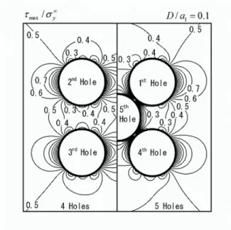
Fig. 10 shows the distribution ofτmaxfor the case of four holes (left figure) and five holes (right figure) underσ∞_y. In the case of five holes, these radii are all same and the interference

Fig. 9 Distribution ofτmaxfor the case of three rigid inclusions underσ∞_y.

D/a1with each other is 0.1. And the geometry in the case of four holes is the same as in the case of five holes. From the disturbance of five holes, we can observe the concentrated stress at±45◦at the 5th_{hole at center. Subsequently, Fig. 11 shows the same geometry for the rigid} inclusions.

Fig. 10 Distribution ofτmaxfor the case of four and five holes underσ∞_y.

Fig. 12 shows the distribution ofτmaxfor the case of seven holes (left figure) and seven rigid inclusions (right figure) underσ∞_y. These radii are all same and the interference D/a1 with each other is 0.1. In the case of holes, we can observe the concentrated stress horizontally (0◦, 180◦). And in the case of rigid inclusions, we can observe it as±60◦for each of the 7th inclusions.

Fig. 11 Distribution ofτmaxfor the case of four and five rigid inclusions underσ∞_y.

4. Concluding Remarks

In the present paper, we examined the in-plane problem of a two-dimensional isotropic matrix containing many circular holes or rigid inclusions subjected to arbitrary loading and produced the general solution to find the stresses and displacements. The purpose of this characteristic study was to apply the Moriguchi’s reflection principle. Using these solutions, several numerical examples were presented graphically.

These problems have been solved using different numerical analysis methods such as the finite element method (FEM) and the boundary element method (BEM). However, our studies were developed in order to observe the interacting disturbances for many circular holes with high precision.

Our next project is to produce the general solution for many elastic inclusions inside a matrix.

References

( 1 ) Moriguchi, S., Two Dimensional Elastic Theory (in Japanese), (1956), pp. 1-77, Iwatani Ltd. (I.S.Sokolnikoff:Mathematical Theory of Elasiticity, McGraw-Hill,(1956), Chap5) ( 2 ) Honein, E., Honein, T., and Herrmann, G., ON TWO CIRCULAR INCLUSIONS IN

HARMONIC PROBLEMS, QUARTERLY OF APPLIED MATHEMATICS, Vol. L, No. 3 (1992), pp. 479-499.

( 3 ) Hamada, et al., A Numerical Method for Stress Concentration Problems of Infinite Plates with Multiholes Subjected to Uniaxial Tension - 1st Report, Transactions of the Japan

Society of Mechanical Engineers, Vol. 36, No. 288 (1970), pp. 1336-1339.

( 4 ) Hirashima, K., and Sugisaka, N., Analytical Solution for Out-of-Plane Problems with Two Circular Elastic Inclusions, Transactions of the Japan Society of Mechanical

Engi-neers, Series A, Vol. 60, No. 575 (1994), pp. 71-77.

( 5 ) Kimura, K., Hirashima, K., and Hirose, Y., Analytical Solutions for In-Plane and Out-of-Plane Problems with Elliptic Hole or Elliptic Rigid Inclusion and Their Applications

Transactions of the Japan Society of Mechanical Engineers, Series A, Vol. 58, No. 555

(1992), pp. 94-100.

( 6 ) Hirashima, K., Miyagawa, M., and Nakane, S., Analysis of Antiplane Problems with Singular Disturbances for Isotropic Elastic Medium Having Many Circular Elastic In-clusions, Transactions of the Japan Society of Mechanical Engineers, Series A, Vol. 64, No. 623 (1998), pp. 143-150.

( 7 ) Miyagawa, M., Suzuki,T., and Shimura, J. , Analysis of In-Plane Problems with Singular Disturbances for Isotropic Elastic Medium Which Has Two Circular Holes or Rigid Inclusions, Transactions of the Japan Society of Mechanical Engineers, Series A, Vol. 75, No. 750 (2009), pp. 150-157.

( 8 ) Miyagawa, M., Tamiya, T., Shimura, J., and Suzuki, T., Analysis of In-Plane Problems for Isotropic Elastic Medium Which Has Two Circular Elastic Inclusions, Transactions

of the Japan Society of Mechanical Engineers, Series A, Vol. 76, No. 762 (2010), pp.