二脚ロボットを用いた人の Split-Belt Treadmill 歩容適応モデルの提案

二脚ロボットを用いた人の Split-Belt Treadmill 歩容適応モデルの提案

音 田 裕 史

電気通信大学

2009 年 3 月

二脚ロボットを用いた

人の Split-Belt Treadmill 歩容適応モデルの提案

音 田 裕 史

電気通信大学大学院情報システム学研究科 博士（工学）の学位申請論文

2009 年 3 月

二脚ロボットを用いた

人の Split-Belt Treadmill 歩容適応モデルの提案

博士論文審査委員会

主査 高瀬 國克 教授

委員 田中 健次 教授

委員 出澤 正徳 教授

委員 阪口 豊 准教授

委員 明 愛国 准教授

著作権所有者

音田 裕史

2009

Proposal of Gait Adaptation Model in Human Split-Belt Treadmill Walking Using a 2D Biped robot

Yuji Otoda

Abstract

Recently, there have been several trials that use robotics as a tool for neuroscience, especially in locomotion studies. In the case of bipedal locomotion, human walking has been investigated extensively over several decades.

A number of studies have measured kinematics, dynamics, and oxygen uptake while a person walks on a treadmill. In particular, during walking on a split-belt treadmill, in which the left and right belts have different speeds, remarkable differences in kinematics are observed between normal subjects and subjects with cerebellar disease.

In order to understand mechanisms behind such phenomena, it is useful to construct the control model of human walking, simulate it using a musculoskeletal model and compare the simulation results with the results of human experiments. But since it is difficult to simulate friction, collision with ground, effects of elastic materials and so on, we would like to carry out experiments using a real machine (robot) rather than computer simulations.

In order to construct a gait adaptation model of such human split-belt treadmill walking, we proposed a simple control model and developed a new 2D biped robot walk on a split-belt treadmill. We combined the conventional limit-cycle based control consisting of joint PD-control, cyclic motion trajectory planning, and a stepping reflex with a newly proposed adjustment of P-gain at the hip joint of the stance leg.

The data obtained in experiments on robot (normal subject model and

cerebellum disease subject model) have highly similar ratios and patterns to

data obtained in experiments on normal subjects and subjects with cerebellar disease carried out by Bastian et al. We also showed that the P-gain at the hip joint of the stance leg was the control parameter of adaptation for symmetric gaits in split-belt walking and that P-gain adjustment corresponded to muscle stiffness adjustment by the cerebellum.

Consequently, we successfully proposed a gait adaptation model for human

Split-belt treadmill walking and confirmed the validity of our hypotheses

and the proposed model using the biped robot.

二脚ロボットを用いた

人の Split-Belt Treadmill 歩容適応モデルの提案

音 田 裕 史

概要

近年，神経生理学における研究のツールとしてロボットを用いる試みがあり，

その中で歩行に関する研究がいくつか行われている．二脚歩行に関しては，数 十年にわたり人の歩行についての調査が数多くなされてきており，人のトレッ ドミル歩行における運動学，動力学，代謝研究などが数多く報告されている．

本研究では，左右のベルトの速度が異なる

split-belt

型のトレッドミルでの歩行 パターンの適応現象に注目する．そこでは健常者と小脳疾患患者のあいだに運 動学的パターンに大きな相違が現れ，この現象の背後にあるメカニズムを解明 することが課題となっている．

このような問題の研究においては，従来，筋骨格系モデルを用いたシミュレ ーションを行いその結果を人の歩行実験結果と比べることが行われてきた．こ のアプローチは簡便であるが，地面との摩擦や衝突・伸縮素材の影響などを完 全にモデル化しシミュレーションに反映することは困難である．本研究では，

二次元二脚歩行ロボット「鉄郎」を開発し，物理的な人の歩行モデルを構成す ることで，split-belt上での歩行パターンの適応現象を検証する．

本論文では，最初に健常者と小脳疾患患者の

split-belt treadmill

歩行の実験 結果を紹介する．次に，関節での

PD

制御・脊髄における周期的な運動生成を 規範とした倒立振子に基づく軌道計画・脳幹における制御を規範とした遊脚着 地角制御（ステッピングリフレックス）から成る従来のリミットサイクルを構 成する制御手法について述べる．また，split-belt treadmill 上件での自律的な 適応歩行を実現させるために鉄郎に導入した，小脳における運動調節を規範と した支持脚腰関節における

P

ゲイン調節を提案する．最後に，鉄郎と人(健常者 と小脳疾患患者)の歩行パターンを比較し，提案した制御モデルの正当性につい て議論を行う．測定された指標の比率と歩行パターンの高い類似性は，筆者の

提案した仮説・モデルが正当であることを示唆していると考える．

人の

split-belt treadmill

歩行実験を行った

Bastian

らは，脊髄・脳幹・小脳・

運動皮質を含んだ神経構造がさまざまな運動適応の制御を担っていると示唆し ている．しかしながら，どの神経構造がどのような種類の調節メカニズムによ りどの適応機構に貢献しているかは明確に知られていないと言及した．そこで，

筆者は，split-belt treadmill 上の二脚歩行に対する調節メカニズムを提案し，

健常者や小脳疾患患者の歩容適応モデルを構成し，

2

次元二脚歩行ロボットを用 いて構成したモデルの正当性を検証した．ロボットの実験で得られたデータが 人の実験で得られたデータに近いパターンを示したので，筆者の構成したモデ ルが二脚歩行における人の神経構造と類似している可能性を示している．

Bastian

らは，以下の二つの調節機構が人の

split-belt treadmill

歩行におい て存在すると示唆している．

(a)

脊髄や脳幹における感覚的フィードバック適応機構(ストライド長やデュー ティ比を調節する

intralimb coordination

に相当)．

(b)

小脳における予見的フィードフォワード適応機構(ステップ長や両脚支持期 間比の差を調節する

interlimb coordination

に相当)．

歩容適応モデル図

それに対して，筆者の提案したモデルにおける適応機構

(

前頁のモデル図参照

)

は，

Bastian

らが提案した調節機構と異なり以下のように要約される．

[a]

デューティ比はおおむね運動学的拘束により受動的に調節される．

[b]

ステッピングリフレックスは

interlimb

コントロールであるにもかかわらず，

intralimb index(ストライド長)を調節する(脳幹における感覚的フィードバック

適応機構に相当)．

[c] P

ゲイン調節は

intralimb

コントロールであるにもかかわらず，ステッピン

グリフレックス(interlimbコントロール) と組み合わさり

interlimb indexes(ス

テップ長と両脚支持期間比の差)を調節する(小脳における感覚的フィードバッ ク適応機構に相当)．

筆者は神経生理学における知見を基に人の

split-belt treadmill

歩容適応モデ ルを構成し，

2

次元二脚歩行ロボット「鉄郎」を手段として用い，モデルの正当 性を歩行実験により検証した．構成した歩容適応モデルと

Bastian

らによって 行われた健常者や小脳疾患患者における実験結果に比率とキネマティクスパタ ーンにおいて高い類似性が見られた．これは，構成したモデルが正当であるこ とをほのめかしている．

また，支持脚腰関節

P

ゲインが

split-belt treadmill

歩行における対称性を有 する歩容適応の制御パラメータであることと，Ｐゲイン調節は小脳による

physic

な筋肉の剛性調節に相当することを示した．したがって，筆者は人の

split-belt treadmill

歩行における歩容適応モデルを提案し，二脚ロボットを用

いて構成した仮説とモデルの正当性を確認した．

1

10

1.1 . . . . 10

1.2

^!

. . . . 11

1.2.1 ZMP

"$#$%$$ !

. . . . 12

1.2.2

&')(+*-,/.021354768$$ !

. . . . 17

1.3

92:+4762;$<=

. . . . 21

1.4

><=?@/A

. . . . 22

1.5

>B$CD1$3

. . . . 23

1.6

^EGFHI

. . . . 24

2

^JK

Split-Belt Treadmill

^LGM-K NOQP L$RST+UVWKYXGZ

27 2.1

^{[]\$^_}

. . . . 27

2.2

^[]\?`

1

^aGb$c$d

Split-belt treadmill

^a

. . . . 30

2.3

^[]\?`

2

aGe$fgh$h$d?

Split-belt treadmill

^a

. . . . 34

2.4

iGjkmlno.7p$q

. . . . 37

3

^{rstvuQw?x y{zm|$}}

39 3.1

~5mD€$1‚„ƒ…

. . . . 39

3.2

^{$‡†‰ˆŠ‹}

. . . . 44

3.3

Œ$Ž$$$‘?D’‡“/!

. . . . 47

3.4

^{”?57•,2€$1}

. . . . 48

3.5

^–$—˜?D_™

. . . . 49

4

^zm|K

Split-Belt Treadmill

^LGM

50

4.1 Tied-belt treadmill

^[5\

. . . . 50

4.1.1 PD

^$

. . . . 50

4.1.2 Split-belt treadmill . . . . 50

4.1.3

š›œ3‚„ž[]\

. . . . 52

4.1.4

Ÿ‰ $¡‘‚£¢¤•¥G_$¦

stepping reflex . . . . 60

4.2 Split-belt treadmill

^$[]\

. . . . 62

4.2.1

^iojk?¦

P

^§]*¨ª©«

. . . . 62

4.2.2

^b$c$dmlnG.

. . . . 64

4.2.3

e$fgh$hdmlno.

. . . . 71

5

^¬G­

74 5.1

€$1D®¯m°o68$ !5±mD²$³$‘

. . . . 74

5.2

^iGjkmlno.

. . . . 76

5.3

´]µ.¶2·$¸•¹º

. . . . 78

6

^»-

80

7

^{¼G½mK•¾5¿}

82

À

¬]Á]Â

86

1.1 General classification of bipedal walking control method. . . . . 12

3.1 Implemented sensors and the usages. . . . . 40

4.1 Desired trajectory of each joint in the stance-swing state. . . . . 54

4.2 Desired trajectory of each joint in the landing-exchange state. . . . . 55

5.1 Specific const of transport and Specific mechanical cost of transport for selected land vehicles. . . . . 79

7.1 Values of the parameters used in experiments with Tetsuro. SSS and LES mean the stance-swing state and landing-exchange state, respectively. . . . 93

7.2 Condition of flotage phase. . . . . 100

7.3 Condition of single stance phase. . . . . 101

7.4 Condition of double stance phase. . . . . 101

1.1 Photo of ASIMO. . . . . 13

1.2 Photo of QRIO. . . . . 13

1.3 Dynamical model of ZMP based control method. . . . . 14

1.4 Setting of ZMP reference. . . . . 15

1.5 Definition of ZMP. . . . . 16

1.6 Photo of Biper 3. . . . . 18

1.7 Photo of bipedal hopping robot of Raibert. . . . . 18

1.8 Photo of Wisse’s 3D bipedal walking robot “Flame”. . . . . 18

1.9 Photo of Endo’s bipedal walking robot. . . . . 20

1.10 Photo of Geng’s bipedal walking robot. . . . . 20

1.11 Photo of 3D passive dynamic walking robot of Collins. . . . . 21

1.12 Photo of Ono’s bipedal walking robot. . . . . 21

1.13 SLIP model. . . . . 22

2.1 Three stages in experiments of split-belt treadmill walking. . . . . 29

2.2 Definitions of the stride length (left) and the step length (right). The stride

length is defined as the distance traveled by the ankle joint of one leg from

the instant of lift-off to the instant of foot contact of the leg. The step length

is defined as the distance between positions of the ankle joints of swing and

stance legs at the instant of foot contact of the swing leg. . . . . 29

2.3 The stride length (A) and the duty ratio (B) in normal subject split-belt treadmill walking are shown, where speed of belts were 0.5 m/s at both left and right belts in the baseline stage, 0.5 m/s at the left belt and 1.0 m/s at the right belt in the adaptation stage, and 0.5 m/s at both left and right belts in the post-adaptation stage. Speed of the fast belt is also shown

(modified from Morton et al. 2006 [Morton:2006]). . . . . 31

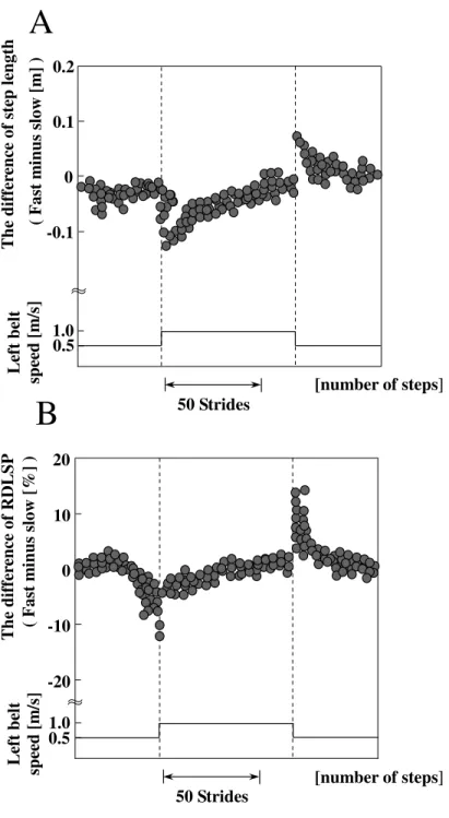
2.4 The step length difference (A) and RDLSP (ratio of the double legs stance period) difference (B) in normal subject split-belt treadmill walking are shown. The time course of belts speed is described in the caption of Fig- ure 2.3(modified from Morton et al. 2006 [Morton:2006]). . . . . 32

2.5 Snapshots on human (normal subject) split-belt treadmill walking in the adaptation stage (captured from Morton et al. 2006[Morton:2006]). . . . . 33

2.6 The stride length (A) and the duty ratio (B) in cerebellar disease subject split-belt treadmill walking are shown. The time course of belts speed is described in the caption of Figure 2.3(modified from Morton et al. 2006 [Morton:2006]). . . . . 35

2.7 The step length difference (A) and RDLSP difference (B) in cerebellar dis- ease subject split-belt treadmill walking are shown. The time course of belts speed is described in the caption of Figure 2.3(modified from Morton et al. 2006[Morton:2006]). . . . . 36

2.8 Control diagram of biped robot split-belt walking. The stepping reflex acts as interlimb control since hip joint angle of the swing leg is adjusted by ankle joint angular velocity of the stance leg as described in Section 4.1.4. P-gain adjustment acts as intralimb control since P-gain at hip joint of the stance leg in the next stance phase is adjusted by hip joint angle of the leg at last lift-off as described in Section 4.2.1. . . . . 38

3.1 Spec of Tetsuro. . . . . 41

3.2 Photo of Tetsuro. . . . . 42

3.3 Photo of ankle joint, foot and contact sensors beneath the sole. . . . . 43

3.4 Mechanical draft of Tetsuro. . . . . 43

3.5 Photo of controller for Tetsuro. . . . . 45

3.6 Diagram of controller for Tetsuro. . . . . 45

3.7 Experimental environment of Tetsuro. . . . . 46

3.8 Photo of knee joint. . . . . 48

3.9 Definition of coordination for Tetsuro. . . . . 49

4.1 Coordinate system in the single leg stance period. . . . . 51

4.2 Split-Belt treadmill equipped with force sensors. . . . . 51

4.3 Inverted pendulum as a simplified model of Tetsuro. Although the sole of the stance leg rotates with respect to the ground in Tetsuro (Figure 3.3), we ignore such effect in this model. . . . . 53

4.4 The knee joint is free to utilize natural dynamics in the swing leg. The stance leg becomes a single link inverted pendulum with virtually passive spring-dumper in the stance leg of steady walking. . . . . 54

4.5 When the swing leg touches the ground (a), the double legs stance period appears. Here, we still call the forward leg as “swing leg” and the backward leg as “stance leg.” The knee joints of swing and stance legs are mechanically locked. In addition, the desired trajectory as kick motion is given to the ankle joint of the stance leg (b) to help the body move forward only in the transitional walking. . . . . 55

4.6 Overview of planned motion and real motion. SLSP and DLSP mean the

single leg and double legs stance period, respectively. The timings of landing

on and lifting off ground depend on the relation between the real motion of

Tetsuro and ground. In this figure, the SLSP starts a little delayed from the

start of the stance-swing state, and ends much delayed from the end of the

stance-swing state. The time t in Table 4.1and Table 4.2is reset to zero at

t = T ⁰ + ∆T , and stance and swing legs are exchanged. . . . . 56

4.7 Experimental results of robot tied-belt treadmill walking with the belt speed: 0.15 m/s. The stick diagram (A), and motion of a foot (B) in landing (a), stance (b)∼(e) and liftoff (f) are shown. The distance was calculated using mea- sured joint angles and the body pitch angle. Of course, Tetsuro moved forward or backward a little on the treadmill, and belts moved to backward. 57 4.8 Experimental result of tied-belt treadmill walking with the belt speed : 0.20

m/s using PD control and trajectories described in Section 4.1.1 and 4.1.3. 58 4.9 Snapshots on tied-belt treadmill walking with the belt speed: 0.15 m/s. . . 59 4.10 Stepping reflex. The robot changes the touchdown angle of the swing leg

according to the ankle joint angular velocity of the stance leg. . . . . 61 4.11 Experimental result in tied-belt treadmill walking with the belt speed: 0.20

m/s to see the effectiveness of a stepping reflex against disturbance. . . . . 61 4.12 Definition of ψ of f . . . . . 63 4.13 P-gain adjustment for split-belt treadmill walking. . . . . 63 4.14 The stride length (A) and the duty ratio (B) in normal subject split-belt

treadmill walking are shown, where speed of belts were 0.5 m/s at both left and right belts in the baseline stage, 0.5 m/s at the left belt and 1.0 m/s at the right belt in the adaptation stage, and 0.5 m/s at both left and right belts in the post-adaptation stage. Speed of the fast belt is also shown (modified from Morton et al. 2006 [Morton:2006]). . . . . 66 4.15 The stride length:(A) and the duty ratio:(B) in split-belt treadmill walking

of normal subject model are shown, where speed of belts were 0.15 m/s at both right and left belts in the baseline stage, 0.15 m/s at the right belt and 0.30 m/s at the left belt in the adaptation stage, and 0.15 m/s at both right and left belts in the post-adaptation stage. Speed of the fast belt is also shown. . . . . 66 4.16 The step length difference (A) and RDLSP (ratio of the double legs stance

period) difference (B) in normal subject split-belt treadmill walking are

shown. The time course of belts speed is described in the caption of Fig-

ure 2.3(modified from Morton et al. 2006 [Morton:2006]). . . . . 67

4.17 The step length difference (A) and RDLSP (ratio of the double legs stance period) difference (B) in split-belt treadmill walking of normal subject model are shown. The time course of belts speed is described in the caption of Figure 4.15. . . . . 67 4.18 The ψ of f :(A) and the hip joint p-gain in the stance phase k _{h p} ^st :(B) of both

fast and slow legs in split-belt treadmill walking of normal subject model are shown. The time course of belts speed is described in the caption of Figure 4.15. . . . . 68 4.19 The measured and desired hip joint angle of the fast leg in the adaptation

stage of split-belt configuration. . . . . 69 4.20 Snapshots on Tetsuro (normal subject model) split-belt treadmill walking in

the adaptation stage. . . . . 70 4.21 The stride length (A) and the duty ratio (B) in cerebellar disease subject

split-belt treadmill walking are shown. The time course of belts speed is described in the caption of Figure 2.3(modified from Morton et al. 2006 [Morton:2006]). . . . . 72 4.22 The stride length:(A) and the duty ratio:(B) in split-belt treadmill walking

of cerebellar disease subject model are shown. The time course of belts speed is described in the caption of Figure 4.15. . . . . 72 4.23 The step length difference (A) and RDLSP difference (B) in cerebellar dis-

ease subject split-belt treadmill walking are shown. The time course of belts speed is described in the caption of Figure 2.3(modified from Morton et al.

2006[Morton:2006]). . . . . 73 4.24 The step length difference (A) and RDLSP difference (B) in split-belt tread-

mill walking of cerebellar disease subject model are shown. The time course of belts speed is described in the caption of Figure 4.15. . . . . 73 5.1 Torque pattern of Tetsuro in tied-belt treadmill walking with the belt speed: 0.20

m/s. . . . . 75 5.2 Specific const of transport for selected land vehicles (modified from Gregorio

et al. 1997[Gregorio:1997]). . . . . 79

7.1 Trigger to walk. . . . . 94

7.2 The floor reaction force. . . . . 95

7.3 First step. T ¹ is the period of stance leg. . . . . 96

7.4 Second step. T ² is the period of stance leg. . . . . 97

7.5 Flotage phase. . . . . 99

7.6 Single stance phase. . . . . 100

7.7 Double stance phase. . . . . 101

7.8 Results of robot (normal subject model) experiment. The ψ of f :(A) and the hip joint p-gain in the stance phase k _{h p} ^st :(B) of both fast and slow legs in split-belt treadmill walking are shown. The time course of belts speed is described in the caption of Figure 4.15. . . . . 103

7.9 Mechanical draft under knee I. . . . . 104

7.10 Mechanical draft under knee II. . . . . 105

7.11 Motor driver of circuit diagram. . . . . 106

1

1.1

^{Ã ÄÆÅ Ç}

ÈGÉʪËYÌ

œoÍYÎ7DÏÐ6Ñ<o=-YÒGÓ/.ԁÕ×Ö5Dm-Ø0ÚÙÛ$¦2Ü5ÝYÞ$ß$6

[Schaal:2008]

^à

áâäã

•<]=‡•f-å

Ë]Ì]æç

(

^è+éYÓm7¨

)

-êë$è]ì]‹?0HíG46¦ 5•mî

â

Ö5Û76•à

`•ÜÝ5mïD5‡59Y46D<=7Þ]Ûñð£ò]óYmî

â

Ö-Ûm6•à

Ijspeert

^{ã ôõln$.0/1}

3öÕø÷YùöÕ¦•(Ô¨†úvû$û2üY%ý0/Ù-ÛG֕þ]ÿ-ó

ã

¥G_ø0ø[äÕøÖ]Û-6

[Ijspeert:2007, Ijspeert:2008]

^à

Maufroy

^{ã YµD}

ËoÌ

lYn•.ԁ Y˜?0ÚÙ$Û¦o†-'ªéªÓ

†-úרv0תÖGÛ6

[Maufroy:2008]

^{à GYom}

Ê YÉ

/î]¦7øG+DòÛÖï

A8©

â

Ö D¦Dà"!#

ã

$?%'&()$å‰+*+

Ê-,.

_Gco0/021Î7AG8H3

ÕÑÖ$Û6

[

^!#

:2006]

à-?ñ'54Ñ'ý.‰G7•Ï]Ð$6768oÎ

Ê

891Î

Ê2:;<>=?

@/ªÞ

A

ðCBEDF

â

ÖÛ56

[Reisman:2005, Morton:2006, Giese:2007]

àHGEI$d7'JK5L>M2NEO

¢G¤$EPQ?©åRS'T]4+6/¥o_G¯?HE35Þî

â

ÖÛ56

[Rogers:2003, Spek:1999]

^à

á2â ã

D<$=?Ô&VUFW?&£Š5Ó]†ú•¨YXEZ-±mDkÙ+¦ ]î

â

ÖÛ-6à•®

ÊE[\

^]

. ¡‘-Þ`_-6

split-belt

a9bc59de‰Ó?¨D/j]k02©gf?6

Ê

bc$d‚„e$f$gh

h$dc-'68ÎAhdie‰Ó?¨v>jkhHlm7Þ`

â 6

[Morton:2006]

^à

D[]\7YÏÛGÖ Ên

oHck/8+°5pv$-މ5î

â

ÖÛ-6ó5

Ê

REqr9stmó

ã

>uv‡>w ãhx

60$y ۉà

á

9z?>{$ß]6$êYëGèì$‹+02H?íY476o¦ $

Ê

9

˜mlnG.0/Ù-Û¦]†7'é@ÚÓ]†ú•¨‰027Û]`|E}Q0-$[]\|E}ñY~9f?6

á

ÚÞ[



Ac-ß]6àÔÕøóÕ .€

8‚]åƒE„ …‡†ˆ

;E‰

>Š‹0i/v0G†7'‰é@ÚÓ 4?6

á

ÑÞ

Œ

c]ßk

Ê

óò

áøâ ã

Ž•*^‘h’vˆ“'”•–ÏÛoÖh—˜–2NEOcg™gš'›œž$chŸ¡ +“H¢

£E¤@¥¦g§¨h©ª«¬'­E®@¥7¯°²±³£´gµ

šž¶$–$·¸g¹™9š5¶7º»¼›'½E¾¿2À@šÁ  Ã

split-belt

ÄEÅÆ¿2ÇEȔEÉ^ÊˏÌÍ`ο'ÏÐ

¥

•5Ñ

¨§

šÒ¿'ÓÔ@ÕΏÖEד

´ØÙ

Ɠ'Ú

Û

¼Ü

¤

¿^Æ¢"ÝÓEԏ¹`Þ ¿>ßàÆg™š'›YÇÈᕖâ5ã

¨

“H¢

Bastian

^Ü

[Bastian:2008]

¹

SLIP

^{ÌÍ^Î}

¥$¦g§^¨

split-belt treadmill

^{äE¿^ÌÍ^Î}

¥

ÏÐåã^æç^¶Vßà

¨§

š$›0è"ȔE•

(

^éê

)

^¿

split-belt

ÄŏÆg¿2Ê9ËÌÍο>ÏEЖâ5ã

¨gë

¢9ìEíîÜðï

Grillner

^Ü

¬ñ

–æÃCò

•ö9÷ š`¹¢ ¼HÓÔÆ ì9íøÜ

[

^ì9í

:1999]

¹™9ùiÜY÷ š>›9úøÜ ¢é ê^¿>”•

£gû

ÁåÜðüøÜY÷¼>ÀÚkæ0à ÏÐýã>¼>òþ5ÌÍÎ

¥Eÿ

–

£

ã7¢”9•ÊgË

¥

£´

ã

¨§

š>›¼`¢FžH¿ÓÔ

ëgÿ

¿

ªi¥

ã

¨

Ã

¥

º ã

¨§¬

§

›9œh÷– ã ¨

ÝÓEԏÆ

ë ¢

2

^`¿!

¥

º" ã'¼'ÇȔ9ÉÊ9ËÌÍÎ

¥-¯

°µ

š›

ÝÓEÔÆ ë>¤

Ï «

–$#% ã'¼!

ª ¿

¤

2

^ÇȔ•

ÿ"&& ')(+*,5¥-.

ãY¢!/0¿

”É^ÊEˏÌÍ^Î

(Figure 2.8

⁰¹

)

¥

ÏÐåã+¢œ¿`ÌÍ^Î9¹

ñ

¿æç-–$2

§¨§

šÁ435

µ

š2›

6

¼789::¾0¿>”9•<;= ÌEÍÎ

¥

Ï9Ð

µ

šž¶-¹Æ&>'÷@?`¢"AB

«

–CEDFGC ï”9•

HI&JLK

¿Ë

¦

¹LMNÆ&>š>›

1.2

O P Q R S T U V W X YZ [ \ ]

80

^{^_ÁkÜ}

90

^_a`bMGc`Áed

¨

ÇEÈ

ÿ4GG ë$f@g

c2ÓEÔh$÷¼

[Miura:1984,

^i@j

:1985,

kl

:1989,

^mon

:1996]

^›

90

^+_`Mocp qr¿

ASIMO

^{ïts!uÖ9¿}

QRIO

¬Fñ

¿<vwÖx&y

z|{

ÿL

¹

-}.

h'÷

[

^~€

:1996, Hirai:1998,

^mon

:2004,

^j}

:2007]

^¢ÇÈ

ÿ

¹‚

ƒ «

c>À ÜY÷<„æ çbc

¬ à ¢0â…

ë 6 µ 6 µ† 6 Ñ ¨

>`¼"‡

´ˆt‰

÷ Ü$c_Š‹h'÷<„

óõô

¿>Ç9È

ÿo

Æ ë ¢

ZMP(Zero Moment Point)

¥ŒŽ

¶ã

¨

Ð ã>¼‘oc$’“‹h$”G„

­®

(ZMP

^•–—

)

¥'¦§¨§

„!‡

´ˆt‰

÷ Ü$¿

ÿ ë

¢˜õ 

¬H¤@™

¹š»FÜY÷

¤

ϋ›æݜžŸ ã ¨

>h¼4‡¡ ¢ý¶

§

ç£

Ù

ÁkÜVÚa„ ¶ ¢¥¤¦Æg¿ ¢

±

á¢9¢§¨©@ª¢}«

ÜY÷¼¬­Æ¿4®¤¦ ¢

¬ñ2ë>£´

Æa>

¨§

„¶$¯

Ø

cH¢

£°±

c>Ú ÜY÷<„$œž

¬

¬­

²

¿'ÊgË

ë ¢ ¤

Ïï

­9® ¬ñ

¿>þ³c5æ0Ý´µ&c¶4·Æe¸+„‡¯

Ø

c!¹»º¼

×c

§¨½ª¾¿¥À+Á4Â

w"ÃgÖ»Ä^¿àƚÅÆîã

¨

à ¢ 

Ðh>÷<„ÇÈ¿ÃgéhÎ&ÉbÊ˹

æ § ¶ ë§

»

¬E§

‡ 6

¼h¢¹}œžÆe¸+„

‰

¶}›¡·

Ù

Æe¸+„!‡

Ì

÷€c! ã ¨ ¢ ¤

Ï¿ÍÎgïÏeÐ

¥Ñ

ÊÒ

¦

ã7¢9Æ&>„« à ÀÁ4Â

w"ÃgÖ@Ä^¿

Î ÁÓ

Ð ¥ 7‹h

ô µ „ ‰

¶"ÆÃgéhÎaÉbÊË0¿Ô

§

 ¢

¥£9´µ

„$

­9®

¹e¸+„‡

‰

¿

­9®

cæ0Ã



Ðh'÷<„$ ¢

ë 'ÖÕÂ

w×>Îor

z

ՋØÁ

º ¥ Ò ¦

ã>¼! ¢

,

¶bÙ?^÷

¨§

„!‡

Ì

¿!_Š

«¬Ú ë

¢

ÀÁÂ

wÃÖeÄ

¥ÜÛ

¼

¬§H¤

Ϗ¹"Ý

¥"Þ

„ßÈ ¢Æ+¸„

[Collins:2001]

^‡

¤

Ï¿

Û»à

r z

ՋØÁ

º

¥bág¦

Æ&>„$ÇÈ

ÿ Vë

¢âã

¬

ÆLÊË

«E¬

 ¢

¥£´

µ „ ‰

¶c2Êîã

¨g§

„!‡

ÿ}

¹ÇÈ ¢

¥ ¢ ç¼ä9¿

­®

¶Eã

¨ ¢

➀

^{åæ « c4ç¹Lè+éýã ¬E§ ‘ ¥b}

Ðýã

Ì

¿4‘

¥

’+“th”G„

­9®

¶Y¢

➁

^{g¢ ¤ Ϗ¢¬­} ¥$½5¨}ê<g

"çac5æÃC

Ø ìë

z Î ÏÐ „ ¹e¸+„‡L˜îí ¬­ac'ÊË „¼äc ¾0¿ ¹hÊîã

„¶ñðòí

ë

º9»@„‡óC

Øôë

z Á Î ¥

Ï9Ð

µ

„¶b¯

Ø

cÊË

«

ÆhÊË

«E¬

 ¢

¥£´µ

„¼ä+cH¢õC÷öø



Ðùïú

ª

¶'¿û@>ýüà

¤@™ ¥'¦§

¼Óԏ¹

§ ô¥à

Áe¸+„

[Taga:1991,

þ"ÿ

:2003, Endo:2004,

l

:2005, Aoi:2005, Geng:2006]

^‡

´µ

„>ÇgÈ

ÿ}

¿+

­®@ë

¢

ZMP

^•+–—e+

­®

¶€C

Ø ë z Á Î ¥

ÏÐ

µ „

­®

c æ Ì

h'÷<„

(Table 1.1

⁰¹

)

^‡4/

ë

ZMP

^•–—

­9®

›<C

Øoìë

z Á

Î ¥ Ï9Ð

µ „

­9®

›

¦§

„ ‰

¶"¹Æ&>„‡iãÁFã

µ ¢ac

§¨

¢L/

ëLÕÂ

w×Îor

z

ÕØÁ

º

¥bᦵ

„¼äcC

Øôë

z Á Î ¥

ÏÐ µ „

­9®i¥>¦§¨§

„0¶

§

ö9÷

¨g§

„

[Miura:1984]

^{‡»@c!ðîí}

ë ¢

ZMP

^•–—

­®

Æ ¬ ô C

Ø ìë

z Á Î ¥

Ï9Ð

µ „ ­

®i¥'¦§¨

¢/¿

split-belt treadmill

 gÉÊËÌEÍÎ5¿ÏÐ

¥

¢Ñ^¼"‡

‰ ÷ Ü

2

 ¢

Þ

cG„!‡

Table 1.1: General classification of bipedal walking control method.

ç

Œ

ç

Œ

ZMP Limit Cycle

‘"!$#&%ñ‘’“ '( ) ÇÈ*Ä+Gq-,!

!.#/%10¢2435 !.#/%10¢27698:

;<=9>?A@ B;<=9>?9@

1.2.1 ZMP

CEDGFIHKJMLKN

OP

ASIMO

^Q

QRIO

RTSUWVX YZ\[]4/^_`a

(Figure 1.1,Figure 1.2

^bc

)

^{dfe^¢}

ZMP(Zero Moment Point)

hgiE%Aj]k7lmWjnop Rrqs/Vht2YhA

(ZMP

^uvw

)

rxy9kyY{z

ZMP

|giI%}fYhA~rxyY67

=€

~^T_` a

7 >A?@

d

U".Y.%ð¢

Figure 1.3

^‚$ƒ|R

€

Yhz„9„]d^¢†…‡fe

2

ˆ‰9Š7‹Œ$%j^_2`farŽ9e{‘A8

’h“

Rr”

’

j|kyY%1•–"fY{z7—˜

’

^T_~`a™RršA›œ

a

TlWž|kyYTŸ^¢ŽA

m

^R¡  

Y|¢A£

%™¤

¥r¦

R‚§©¨9l".Y

>

+ª«a¬4­9‹

(x

^®

)

^{¯d9°$^f%}

€

Y†±

ZMP(zero moment point)

^%|y/ƒz$„

¥

ZMP

^

foot

¥’

RA²¡X³H¢µ´¶e·¹¸¯9.Y„"%

€

[»º¼½j

€

y ¥

d¾9–d"²Y{z¡¿.„hd¢

ZMP

^

A(

  ^/%

)→B(

^À.Á]Â

)

R{Ç"fY"‚.ƒ

€

ZMP

¥Ä

iAo

p/]Åfk

(Figure 1.4-(a)

^bc

)

¢"¿¡XfR^¡_`~a

¥

0Æ

¥

ZMP

|qs/Vht2Y"‚ƒ

€Ç ÈhÉ ¥

Ä

iAoAp¹|lm

·

qs¹VhtX³4¾9–

€

—˜~|0

O

d2¸Y{z„

¥

Ÿ^¢

Ä i

ZMP

^R{­Ê

’h“

±

¥{Í

€ ÈhÉ

(C )

¥ @

Ñ9R.‚Ök7Ç/V{t X$³ y d¢¡´.Î Re ¸ +.ÕhÙÚK%†YzÁ

nH¢

ZMP

^{6ÛAÜÝ

¥

foot

R{ÞA0R{Þß"fYnAÌR¢à%§™á

×

ZMP

|giI%}fYh~]˜

ƒãâ"ۗ"˜.d$e

foot

^e

Í

¸~[

€"×

X$³

€¹Øh€

y

(Figure 1.4-(a)(b)

^b"c

)

^z

foot

^¤\[

€

Y%

Û ¥

¢£

>

+ª$«¹a©

Í

¸[

€

YnAÌR

,

^ä

ÈhÉ ¥å

›"æ

Í

¸[4j|k

Í ¸ € a @

Ñ]¨l

Vrt2Y{ÙÚ.²"Yz&j] ¹j7¢f¿ƒ}Y2%ãç~R

ÈrÉè

›œeé/V [

€

Y9nÌTêë.yT‡/¸d

Ä

iAoAp Rhqs¹VhtY„"%-ìíR

€

Y{zî¯

¥

± 

Ø

êëy4‡¹¸9ï]ÙAÚE%}ðfYh‡A—˜2RAeH¢

ñò =

RóAyAky

€

y7zÁ9nh¢ôõö÷ø RùyAk

¥

­Ê"ú

’r“

±

¥û ü

¢&ý$§ãá

×

ôAõ

öþÿ. „ýR.‚AÖk$á Ök¹jTÁ~ƒT‚fƒ

€

 y ‹ RùyAk

¥û~ü

e Í

ìTí.d

²"Y9nÌ`¢AôAõö—˜R4óAyky

€

y¹ý

Ø

XYz$¿

¥

RH¢

ZMP

^ï

foot

^Rß/Ökù

[†ReRï7ky$YrÙÚ.² § ¢ï2³7ð½ý±Eýhy&ƒ! $

ü#" €

yTÿ$R

€

Ök/jTÁ ƒ

¥

d¢%'&

¥

‚fƒ

€

ï2³ jn—˜2e

B

R{íIj{y

€)( ¥!*+

4²"Yz

Figure 1.1: Photo of ASIMO. Figure 1.2: Photo of QRIO.

-ma

mg ZMP

x z

Y

a [m/s ] ²

C

A B

Figure 1.3: Dynamical model of ZMP based control method.

x

Forward

Landing leg ZMP reference

(b)

Figure 1.4: Setting of ZMP reference.

ZMP

,#-/.102436578!9;:0<

Figure 1.5

^e

foot

^R¡ù

×

Yú

¥=!>@?

d"²Y{z;A¤2eCB!DA‹E8d/FG@H

€ ¥

d¢´@I

¥

ø/J

¥

Œ#K RL

P

ðY{± RM"xð2Y#NO

€ ú

R

^{ýjhkÁ ýrÌ}

Ø

X2Y4zú/PÑKa

@

R

^Q/R

ðfY„

¥

Mx9±~ï

ZMP

^ýTSU¡z

ZMP

^eCE­Êú

¥’h“

±

(Center of Pressure; COP)

^¿

¥

¥

ýjhk9–!V VXky.Y

[Vukobratovi´c:1972]

z;B/D‹~RW;B.ðY{´fÎ È{É

a @

ÑARf‚Ök

COP

^ïXY R#Z!M"ðfY„"ý- [1\d"²Y{z

5.1

^d¢

COP

ïTZ!M"ðfYh´Î a Ñ úfR]

Ä j

ZMP

^{! ^/_`}

¥ab

ýAj]k

¥c

LœR

È

jhk d¹ïh˜/Ö7nTz

R

ZMP

Figure 1.5: Definition of ZMP.

1.2.2

e)fhgji@k4lnmporqts4uwvyxHKJMLKN z1{@|}~;€‚!ƒ

„

öEj]ky$Y

foot

^MYrZ

è

þ¯R

ZMP

^{ïhß$À~„$ý}

€ [ —˜.7˜"áXYC…ï'¢4¼Å†!‡

>?9@

ýAj]k.Y$„ý†d ¸9Yz4—˜R7ù

×

Y{¼Å!†!‡

>?9@

e

Figure 1.3

^R7ùyk

x

^®

¯9d

A = B = C

^ý

€

Y'¢9À.Á§»ÜÝۈd¡±

C

R¡ùy9k¡±@BöWjY¢

x

®—˜2R{¼"X ‚.ƒ9ý}ð Yr¼Å†!‡Ký

€ § ¢¿

¥

ÁÁ

¥

ÿ!$$d¡º¼ï‰‹Š-nÌR.ƒŒ@Ž

¥

Ûï†\§

ü

j]k7‘ï

ܐ$Yý]y&ƒ …‡¹ï‘G§“’Ej}˜àƒ™—˜ï7y&ƒ z/„

¥

"RC”•"yn! ^/_ïh¼Å!†‡w

! ^/_Eý—–Eƒ z&„

¥

¼Å!†‡ÿ!$$d²Y¡Ÿ¢9ÜÝÛ´$Î ÈrÉ

R7ù

×

YEa

@ Ñ ü

ú.e9°f^

€ ¥ d

ZMP

^eR±

C

^RL

P

ðYz&„

¥

ÿ!$2e—˜

’;˜!™

E!š R7ùykô¾A–$d$²"Yz/j

 ¹j7¢&„

¥

ô¾A–

€

ÿ!$ï]ÜÝÛEý›Û

¥œ!

ï‘M§“’.ð„ý|dŸž `a¢¡£$ÑC¤ ï ò m

j}¾9–¥½j|kyY{zÁnH¢„

¥

@^!_d"e{ÜÝÛ´Î ÈhÉ

ý

ZMP

¥

¾9–¦šï§¨©

Í

¸ª

foot

^«9ڐª

¥¬

¢­®$ïT¯r°ã𩂱"ý­²

¬¨³

©#´

a@b

ý;µT¶·¸C¹º»/¼!½1¾)¿¢²À

Á

°—ªpÂÄÃÆÅÇ»/¼‚ȸÉ;ÊËÆÌÀ

Á

°ÎÍÏ

¬¨³

©C´Ð±Ñ‚Ò

ZMP

ÓÔÕ¨¸CÖ!·'× ØtÙ'¿Ú ÒÛ!ÜÆÝ

¬‚Þ

©´ß)à¶@á âã!äå!Ó!Ô!ÕƸַt×Ø)Ùt¿æÒá

ZMP

Ìçèéڭꐩ#ë!ì»í

î

¬ïtðñ

áò/·ó‚¸/Å#Çõôè!ö÷'¸Cø/ßë!ì@ùÑpÚµ¶ú‹ûýü

³

ªþÿ Ú

ѐ©

ݪ ë!ì@ùÑ1¸

Á

ѐ©

ñ

á×Ø Ù)¿æÒ °Î·)Ìê)±‚Ú ²

¬Æ³

á

Ê õµ¶!©´#"$%

¬

Ґ±¸ë!ì&')Ì()!

ñ

´+*,¨ÝÒ áâã!ä!å»!í î Ì

()!@¶ö÷-.)Ì à ñ

(4.1.3

^Ç/Ü

)

^´

®0

[

^®0

:1981]

Ò12·435687:9  ¸:;@Ê<=?>@à¶A@CBƸCò/·¨¸35;<)Ìëì ê?DEF;ÕÖ!·A'× ØtÙ'¿ G

Biper

HÌ:I+J‹µT¶!KDC´

Biper

^¸L,)MONtÌ

Figure 1.6

^P

ê´

Raibert

[Raibert:1986]

ÒáCQ:ÆÅǨ¸R4S4<T)>DU

Á

¸ëìáV142!·WAS1óXY4,

²+5Z8Ûе¶[\TA]KDK>_^ê_D Y,!ë!ì/á`>aáò·4b5c_dÌUef Á g

D1±‚Ú

K>+D:h_i¼kj á l ÏAf@ë;ì'Ì(X! á

1

^á

2

^á`T>a

4

·Æ×ؐٿθ m4

(

^nÙi!¾Oo

)

^.#pе

¶!KDC´q@¸CÖ!·)nÆÙOi¾+o@× Ø'Ù¨¿ ¸L,)MONtÌ

Figure 1.7

^P‚ê´

Wisse

[Wisse:2008]

Ò áC@Ê<)ÌUe

¶ ôè4@Ê<)Ìr21ê_Dts+u/Ù)¿wvx)y

î

ÕƸַ)×Ø Ù)¿ÌOIJ

µT¶!KDC´)q@¸CÖ!·'× Ø'Ù'¿ ¸L,)MONtÌ

Figure 1.8

^P‚ê´+z4{

[

^z{

:1979]

^Òái/Ù}|

\AZ~C€

Á

Ñá;·S

ÌU2‚Öƒ„=ۆ…U‡;á†s+uÙtˆwv?x)y î?‰

2?‚Cl@Ï

Š

ÌU‹(Œ…

ñ

ëì4„8ŽA‘…

ñ’“”k

[

“#”

:2002]

ÒáKi!ٕ|\CZ–~

‰—K˜)™š

›y|Xœ

Xž)Ÿ

‰

]4!O„=ۑ…U‡ ¡ÆÝ4]K¢£

ž

j¥¤ÐÙOy ¦^+§‚Ú?>=¨Äփ4tU©ª†…‡!

D ’ 7 ñ

áVG¬«­¨®H4¯

‰

ñ

—˜_™š

ˆ î

y4°+±/êTD²³8#‚X!‡)ûµ´¶·… ‡X!?D

’

áC«­¨¹¯=

™ º

…

[Hodgins:1991,

^»8¼

:2005]

^{]t½¾ D}

Figure 1.6: Photo of Biper 3. Figure 1.7: Photo of bipedal hopping robot of Raibert.

Figure 1.8: Photo of Wisse’s 3D bipedal walking robot “Flame”.

ÌÍ

-ÎÏ

‰

›Ð×

ž

|Ñ+Ò

‰

Ó4Ô4Õ¾+Ö×8ۑ…U‡Œ½

‰

>?^ X؂ê_D

‰

T

Ù

…4>_^!Ú êTD$%?¾K]_Ú:ۇK!D

[Takakusaki:2008]

’AÜÝ

[

Ü4Ý

:1997]

^{¾áC-Þ ‰ßà}

á4â

ê?DUãs•ä4å-.4æ

CPG

^{‰ç4èé í î}

[Matsuoka:1987]

 (K!C‡ փA=ê?u:œ?ë

ž

ê–ìOí#.ApîÚ

g

‡4ïðá Üòñ

‰

$%ó)¾8§

‰

>?^]:ôõ4ö!äå()!

ñ:÷

J¨Ý4-

.=ø­¨¹ùú=>?^ A]à ñO’

§

‰û

Î=üôõö!äå

‰ý

þsVäå;áÿ„

‰

þsVä

å áCÖ×éÚ

‰

¯(

‰

sVäå

‰

Xo

ž ¤ î ] GªH J4-ŒÚ

g

D§

>@à:‡?›kˆy

Ÿ

Uö.‚ê_D

[

:2005]

’ q

‰

A…U‡ClÑ !T]:

)¾†s›

î

Ÿ

xAå)-.ÚÛTD

’4Ü4Ý

ü_§

‰

>?^U]

û

Î"$#!

ñ

i%U|#\AZ~:Ñ

‰'&

ƒ48ê_u+œ

ë ž

ê8ì:í+U'à‡!KD

[

Ü4Ý

:1997, Taga:1991, Taga:1995a, Taga:1995b]

’ § ‰

>^µ]

÷ J

Ý 4#-4.)( ë@ì

é í î

ü*)!l+,.-8/ …µ‡A`‘¨¢á

Þ

D10C<

‰2.3

Ó+4+5A5T#ی…µ‡Æû

l‘…

ñ

6

Ÿ#ž

íU-.ŒÚ g D

’879¦

ü;:=<IJ†…

ñ

KYS

äå>1?@#Û?Dôõ öä@åt (K!C‡=iA%}|OZ–~Ñ

‰&

ƒA=ê_uœ=ë

ž

êtìí#U.CpîÚ

g

‡!KD

[

79

:2003]

’

q ‰

äKåtü ÜÝ

é í î

CPG

CB D¦… ‡EEFGH,A-T¾.*

ñJI

*KMLÑ

‰ NAOçQPš

¾

RTS

ÑUXDVXWTY…U‡AZ)D

’

ôõö[\ ]–(ZA‡ ^_–`_ba ©c>A…U‡KüdƒG ef%tˆ

[

^gEh

:2003,

^A

:2002]

¾+ijGkCÑTUl

’ &

ƒ?Ñ)ümAnpo

[Aoi:2005]

^¾©Ac?Ñ

3

^qrstvu

I

wx

o

[

wx

:2004]

^Ó

Geng

^o

[Geng:2006]

^¾+©Ac)Ñ

2

qQr stvuHy'^_t©ªŒÚ8zA{QZl

’w

x o I

Geng

^{o`y &|} ef%f}~y'€TH‚„ƒ.…+ÛT†Û

Figure 1.9

I

Figure 1.10

^‡ˆT‰;Š

Passive Dynamic Walking

‹Œ$MŽ ‘’

Passive Dynamic Walking(

^“H”

PDW)

^•

I—–™˜š›+œMž ŸH˜f¡ ¢;£H¤

‡8¥¦Z.{

McGeer [McGeer:1990]

‡T§M¨ª©«v¬­T®'^_¯Ul'Š

PDW

^{• °c±Vy²T³}

ž Ÿ+˜v¡ ¢ £µ´¶V·¸

¹

Gº

ƒ»¼‰lE½

´

¯°

¸ ¹

„º'¾Q¿MÀ„Á

¯.ÂÃo1Ä ÀAÅ

¨~Æǃ\MkQ‡

Å

l'^A_vƒ+ZÈaªŠ

McGeer

^•;°É

¢š›¸AÊË

ƒF²V® ÌHÍ

´XÎ

‡

passive

ÀAÏ`Ð

ƒ1ÑTÒ®Ó

|

c.±Gƒ8¼QZ.{H°CÔ

Õ¿QÖTÀMÁ

¯H×$Z Ø tT¯y

2

^{qQr.^_‡ÙÚ}

Á ®

[McGeer:1990]

^Š

Collins

^o

[Collins:2001]

^•

… ­T‡Û;Ü݄ƒ1²$³

3

^qQrQÞß



ƒ1àá

Á

®;Š …$½8¯• °;℃1ãfl½

´

‡T§.ä'{

yaw

^åVæç¨

y+æ'èMƒF鄬VêìëÒ °§$¨îí.ïEk ‡FðVñy8^ _$‡1ò$ó'^ _ƒCôõ

Á

{ óQl8Š ö1÷°1Ô ÕÇÁ

{

ó À

óQy+¯ øùyúû‡'üý‰El½

´

•.¯þ

À

óÿ° ^_•Ý€

´

øù

´ ÿ Ö

k‡

áA¼MƒÈ½

Á

° þba ½

´

‡T§ä{‰Elã¯Ql½

´

ƒQ‰El ‡

EÀ

ÙT¯.°! êy#"$&%‡('&)µƒ*+

Á

® Š

Collins

^{,`yÓ |.-0/21 } ƒ}

Figure 1.11

^‡

Figure 1.9: Photo of Endo’s bipedal walking robot.

Figure 1.10: Photo of Geng’s bipedal walking robot.

ˆQ‰;Š43±$y8²Q³

ž;Ÿ ˜„¡¢£

ƒF»¼¯Eþ!5FÓ

|-6/71

}ª•°(8:97;

À(<=

ƒCô.õQ‰>5Q½

´

‡@?

ÁA

ó5

[

^BC

:2003]

^ŠED

<=FH˜šV› œ'Gž Ÿ.˜µ¡ ¢ £

ƒG H‡

Á

®ÓI

<=

Ô Õ

F

":$

´+ÁA

°4JEKL,

[

^JK

:2004]

^•7MON

¸ ¹

$ºQPER:S&T

Ô Õ

ƒ`°4UVEWL,

[

^UVW

:2004]

^•

XY2Z\[ Ê^]`_

1 ¢ Ô Õ2a

©«

Á4A

ó5Šcb.® °

Wisse

^,

[Wisse:2003]

^d:e2fg,

[

^e2f

:2005]

• °Ehi&jðkl

a

¼óA® m

1

š0npo qsr&t

ÓI

-!/u12vxw!y

ó A

°6D

<=2a

G7H w Á

®(89 Fz

ó

<&=.a

ô õ ÁQA

ó{5`Š}|

w

f~L,

[Takuma:2006]

^d!2f,

[Tsujita:2007]

^{•;° v}

€#1 ]C¡ 

Û+¯

_ >F

on/off

FQË;ŸV¡‚ƒ:aQ„.ÐÇÁ'Ï1Ð7F…6†.a

úTÒ\5½

´ w

§E¨

<=E‡

ˆ.a

úûf¬‰®;Š@Š$Ò

A

Chemori[Chemori:2004]

^,1•;°!‹É

‚(Œ

€Ž

n2a

¼ó

A

ô õ

Á ® <

=gF!†pa@‘’ Á@A

ó>5;Š éK^,

[

^éK

:1994, Ono:2004]

^•

Î w É

¢ šV› ¸Ê$Ë&a

ÑVÒQ®

3±¯°:“

‚”:•&–ua

¼ó A v

M¢:—Öca4=™˜ –

Self-Excited Walking

¤a:šE¡ ›

€

ʚ2›

‚

¯!œ

Á

°Hô3¯ ôõ Á4A

ó5#ž éK^,Žd

Wisse

^,

F

3±V• °

McGeer

^ÿ&Ÿ!

Á ®

<=

3

± ´

& 

w(¡

®'±E¢

aÁQA

y

¨J°£¤

F I a

Ó&I

F § ˜ w

áf¬‰75½

´

¯+°

2

^¥¦:§

nuo

¯ F ÓI

<=2a

ôõ Á4A

ó5#ž.éK™,

F

¼TóA®'ÓI&3±

a

Figure 1.12

^w(¨>© žgb.®#ª&¤™,

[

^ª&¤

:2005]

^•@D

<:= F

3:« ; À6

û

F@¬:­

+ÿH°

CPG

´Q®(¯TÀ'¶

(

°²I²±´³I:µ$ñ

)

„ Ð

¯\5½

´6a

¨

Á4A

ó5#ž

Figure 1.11: Photo of 3D passive dy- namic walking robot of Collins.

Figure 1.12: Photo of Ono’s bipedal walking robot.

1.3

¶ · ¸ ¹ º » ¼ ½

½F­>b¯'ð

F@<=

Þ+ß



d!¾

=

Þ.ß

a

±+Ù Á §

˜+´x¿

T§

˜H´

°ÁÀ pê

F

":$Qÿ

À

¬1­

A

ó\5

[

oQÂ

:2006,

^Ã&Ä

:2007]

^ž4ÃEÄÅ,

[

^ÃÄ

:2007]

^d!Æ:ÇL,

[

^Æ&Ç

:2007]

^•@lEÈÉ:Ê

´ÌË:Í

Ê F

0.á.¼

w

§#5}ÎE!+Ù

w

¥¦ó.®Cð

FQ<E= š¡›

€

ÊEš{›}‚aÏ=

ä A

ó&5žÐ

Î

[

^Ð

Î

:2006]

Ñ

°@ÒÞpÓÌÔ Ê £

v F

Õ

PREÖ:×EØÙgaQÚ

óÛÜÝÞßEà

<E=\áâ6ã{F

Î:Þ!ä:åçæ ØÙa

2

¥&¦!§

nco@è\š{é4ê

€ìëLvÏí Aî

5žQï:3

a4Úî

Ûïð

è

Ñ(ñQò róEô

(Figure 4.3

^G:õ

)

^Ñ

<

= w ñ

SLIP

á0âã

(Figure 1.13

^Gõ

)

^{Ñ ¾}

=

wQöuí

A&÷øù(ø#ú!û

w

Ú&îcüxøEAEî&ý

ž

Bastian

ü

[Bastian:2008]

^Ñ

SLIP

á&âEãca(ÚîA

split-belt treadmill

^þ

è{ÿ

¾

á&âEãca

å

í

˜

æ

¿ :îý

ž

Ñ

ß

v

a4Úî

Û

ÿ

split-belt treadmill

á!â0ã{ÿ

å

:îý"!

tied-belt treadmill

Úî ÿ#$ %&

[Hirai:1998, Tsujita:2007, Nomura:2006]

' î)(+*-,.&ý '

ñ/0

ÿ1ý2,4345

split-belt treadmill

^þ7698:

ý

á!â0ã\ÿ;

å<=

îý?>ÿ#7$A@ã

ëCBD

ñ E4F G

è

DHJI

Û

ü"Kî !

L#$7M

6-84:

ý

ßA-NAO ÿP#$

D ñ

2003

^Q

4

^R

5TS)U

!Û

!-VCW

DPX

ÿ4Y"Z\[

ë`_ba

Pc6

ÞAfähg;ijk Al Û

[ :2005]

^D-o

Ø:ó

Þ X

æ"pq

(

^r=sut

)

^v=w4"x

9yCz

iÛ?{7|

ñh}~€

ä&å ‚

CPG(Central Pattern Generator)

^?ƒ

î

C)g;i 4„

æl

C…P!‡† '

ñCˆ‰

í …

A4ï EŠ

ýŒ‹

æ

D9Ž

è

. …!



D

ˆ‰

K

CA4ï EŒŠ

ýŒ‹

æ

'C‘’ è=.\ý

擔

ñ0ò•

ó&ô á&âEã

?ƒ

î…?–

Þäå|A=ƒ

í

…P!

Figure 1.13: SLIP model.

1.4

— ˜ ™ š › œ

L#$ÿ\?[

D ñ

(

^žŸ

0C ¡7¢7£¤7¤70

)

ÿ

split-belt treadmill

^þ

è{ÿ

C

áâ:ã

4ßANAO{7¥ æ í ƒ

î ¦

Š

ýŒ‹

æ

èŒ.\ý2!

ÿ

ÿ?–

Þ§

ñ

Þ¨-§

ñ©

ª4«P¬­

q®

ý…¯

6°O±

_

éÏã

þ

è{ÿ

ï{ð

'²³

( zøî>ý2!9´

6

ñ7µ¶

ÿ ·:ã

O

ÿ?¸C¹

' º K{ý

split-belt

^»¼

è{ÿ

C½A¾ ë¿

ÿ

CAq=®

ý æ ñ

ž7Ÿ

0 æ

¡7¢

£¤7¤0 è D

–CÀ

§ [

½A¾ 뇿

6?ÁÂs KPÃÄ

' E øý

[Reisman:2005, Morton:2006]

!‹6ÿ

ÃÄ2ÿPÅÆ

6

*=Ç

D

2.2

^ȌÉ

2.3

^{È);ÊCËÍÌ}

Ç=…†

s

…Ç!‹ÿ

EÎ ÿ9Ï

6

.ŒÐÑÒ

Ó

~7€

ÔÕ

Š

Ѕ¯

6 D

É-Ö×CØ

XÙÚÛ

?ƒ

ÇC…CÜÝÞ

±ß Ü)à

¿

Ç=áÿâã

\ä2Cåæç

âã°èêé

®

Ќ‹Œè

'

æ4ë

[ì=.Ð2!

Ì ,

Ìkí

è

äîï

 ðñ òôó7õ ª7ö

ä

÷øKJù

Ü4Ý9Þ

±<ß°O

Š

Ð=‹è

'

Ž

ì.CÐ?!4á‹ì

É

L7#$=ì

D

2

úCû-ü7ý7å\þPÿ

O

fÌ<Éæv

·

ß

ì

\ä2Cå

ÙÚÛ

Ì É á ä

ÙÚÛ ' ù

ä

„

6

ÇCÇÐP,

Š

Ð2!U…

¡7¢7£¤7¤70

äå

Ù7ÚÛ

Š

Ќ‹=è ' ì

s PÉ"!

6

}%$'&}  

å(*)+-,.äCƒ s ävä Ì D

É324

5

ÈA6

B ß }

ƒ

Ç4ЋŒè"ì76

ý‡ä89

Ù ß Ñ ¿

O

ì s І

: ¡ g ( Ì

…‹Œè

É

foot

^ä

í:A

¡ g ( Ì 3;

í‡ä

÷7ø

=<\:76 ((

Ì

…‹=è

É?>*@

é

A ( Š

Ќ‹=è<ì 5

ÈN=BDC

, ( Ì

…‹=è

ÉEF

¿7G KAù

ä

ó7õ ªö

H

5

È\6IKJÌ

…‹=è;KAù ' .L

CM

Ð2!"NO

{|

è Ì D

1.2

^È\ä

P è

2.4

^È

ì7Q

®

…RTS

5 É

CPG

^{äUWVX ÙÚÛ}

è Ì

}ê~

Ý

Ò Û

K–CÀTY

f*Zhg;i

Ð[*\

Z

ò^]*_

6 8:

Ð7`a

9 ó

ab*c

ä3U3VX

ÙÚÛ

è Ì ä

5

ȇ68=:

Ð

PD

N*O

òed3f*]_

bc è Ì

d"g

¸¹Íèihj

ä

ˆ‰

Xä …¯

ä

¢k-l"mon

Ð

stepping reflex

^pqCr

Ðs#

ä } Ý

utwvxoy Û Y

*

Š

ÐN*O

{7|

lz

…

l{*|

Ì …

¡¢

l Ð}o~

ä3UVX

Ù7ÚÛ

è Ì

ä€Cý

5 È

lWmn

Ð

P

^{‚Ex ¿Mƒ È}

Y„…"†o‡ˆ‰Š

‹TYŒÇ

É3KŽ

}K~Y…K‰7‘

1.5

’ “ ” • – —

˜™š

ä*›"œKžŸ¡ 

ìE¢K£‘¤

1

^{¥ l"m¦}

›§¨*©ª*«K§

s¬

ž­®¯*°*±

Š‹

ž²*³§E´=µ¶

£=·

¯*¨*©

Y

²*³¹¸

‰º

§ ˜

¨*©ž-»¼E½¿¾oÀ

‰‘¤

2

¥u›Á*Â*ÃÅÄiÆ*ÇÈ É*É

Þ

split-belt treadmill

¯žÊKËWÌÍT½=²*³E¶

£

[Reisman:2005, Morton:2006]

‘uÎ*Î

ÏKÐ"ÑÒÔÓrÕ

split-belt treadmill

^Ö×Å»¸

‰ØÙÚ

ÐÛÜ

½¿¾oÀ

£‘ÝÞWß"à*á

¸ ‰

Ž

}

~âã3ä

Ö"å

¦

ßæç

¶

£‘¤

3

^¥u›è

à

¼Öé*êë¸

ß*ì"í

¸ ‰

­®ïî7ð-ñ-t òôóEõWöoÖ"å

¦ ß

¾KÀ

£‘¤

4

^{¥›§´=÷ Ï ž}

PD

°±ùøûúWüuÖ7ýEþ

£=ÿ

¼

Ð

á

½ ÅÄW¸

‰

Ö ø ÇïÖý?þ

£

°±T½ ĸ

‰

®*× "!°± #

stepping reflex

^$

Ø&%iáT£('*¬

ž*),+ñ.-0/12 ä ½

àá

¶ £

°±

ŠK‹

Öå

¦ ß

¾À

£‘ïÎ

ž

'*¬3

ž°±

Š‹

Ï

¯.4

‰

tied-belt treadmill

^{¯*ÊEËuÖå ¦}

ß65"7

¶

£‘98

¸ ß

§3óoõ?Ö

split-belt

^:";

Ï

ž=<?>u¼ Ð@9A

¯T½=ÊB&C

ˆu£W‰D

ÖE"Fë¸

‰

§"ÆÇïÖýþ

£

GH

÷½I" ĸ

‰

JK

®L-´÷-Ö"ýoþ

£

P-gain

^{H ÷T½NMOo¶}

£‘Î

ž¥užP

º

ÖóEõqÄRQ

(

Á*Â*ÃÅÄiÆ*ÇÈ

É

É Ã

)

^žÊKËWÌÍ

[Reisman:2005, Morton:2006]

½(SUTë¸M§MOë¸

‰

°*±

âã3ä

žV=WIX-Ö"å

¦

ß,Y™

½=¯[Z

‘"¤

5

¥u›§ÊKËWÌÍ-Ö"å

¦ ß

žU\^]T½¿¾oÀ

£‘`_a

C(bcdež^SUf Ähg

i,jlk

žm

¦^n"o

X-›7§

Ò¡Ó

žqp

æ

ÄrMOŸqc

â*ãWä

Õ

V.W

Ï

¢E£?Î

ĽUsž

DWØ

¸ ß ¦

£

ÄN\

Þ£tW¤

6

^¥ïÖÌ

™ § ¤

7

^¥ïÖu

º

žqvw½ ¾?À ßyx

Ä D Ä ¶

£t

1.6

•

^®

—

^Lï´÷

Ø&%

Kž~"

•

JK

®

(

^€

)—

^{"ïւ Õ6ƒ9„ ¸}

ß ¦ £ ®

(

†…

)

•

®

(

^€

)—

^{Ö‚ Õ6ƒ"„ ¸}

ß ¦ Ð ¦ ®

(

†…

)

•

2=)I‡"ˆ

k(‰

—

^®T½

 NŠ"¶9‹Ež3å x·

Är -ž^Œ

•

^Ž")

k 2

—

^‘´÷

Ø&%N’G“

~"

t ‘ ’ ) k 2

•

^¶”)

k 2

—

^‘´÷

Ø&%N•G“

~"

t ‘ • ) k 2

• foot—

^‚–´÷

Ø&%N•G“

~"

t å x·

~DÄ ØØ

Är~'½—G˜™

ß

foot

^̛

•

^ƒ

—foot

^{Õ  Ä ƒ9„ ¶œ(žŸ}

tU y…

•

^

—foot

^{Õ }

Ø&%

bœ(žŸ

tU y…

•

^{‰¡ ñq¢}

—

ÎÎ

Ï£¤¥

Ä¿¶œ

•

^{¤ ¯}

ÿ

—

ÿ

¼

Ðq¤

¯-Ö3ý9¦

ߧq¨9©ª,«“

ž"Ÿ-Ö

Ð œ x Ï

“¬G…`t

2

^{‰¡ ñ¢}

ր=W

•

㝭

jU¡†®

S

—

^{¤ ¯}

ÿ

Ö¯

D œ JK

®€

“°

—

•

^±®

JK9

—

^{±® Õ6ƒ Ÿ}

ß

¦œ

l…

•

^²®

JK9

—

^{²K® Õ6ƒ Ÿ}

ß

¦œ

l…

•

^³

—

^´qµ"¶

“ Ð

¦6·

§

·¸

Ð^¹



•

^º³

—

^{³ »¼}

“ ¹ 

•

^¶

3

—

^{" °*±}

§ è à

Ð=½

Ö"ý"¦

ß ¶

“K

å6¾XT½N¿\EÖ¸

§âã3äÀ

¶yœ

Î Ä

•

pÁ"ÃùøÅÄ

k

g*è

à

—

ÎÎ

Ï£

JK

®‚–?´÷"!

©

øÆ!Ç

© ½

PD

^{°±-ÖyȆÉ}

«a

Ö"¶œ

Î Ä

Ï6Ê"

¼ Ð

ÃùøÅÄ

k

gè

à

ÄIË

Ð ¶ Î Ä

•

^{Ì ¤ ¯}

—

^{¤ ¯=Í ¶*À Öý9¦ Ì-¼Ö^Î Ð žŸT½(Ï=Ð ÐWÕ ¯ÑZ ¤ ¯}

•

^{¤ ¯}

—

^¤ ¯=Í*ÖÌ-¼Öqº9Î a Ð

 y…

Õ,ÒÓ

¶œ

¤ ¯

•

^@A

—

^Ô

Þ.%

bGc»¼K½¿ÊBK¶œ,c

D

Ö¼Õ

“(ÖÀ

Ö

AØ×

ß

"

g

i6jyk

½

ÖÀ

C™

œèÙ

[

^Ú"Û

:1999]

•

^ÜÝ

—

^{Þ"ßà Ï£}

§"á

k

/â

5

Öy-

ä

2Š^ã-½(ÜÝ ÄIš›

•

^{äå^ÜÝ}

—

^¼~

Ø&%“æ"ç

ÖÈ4

ß

ä"è

ÕUéê

§,ë

è

ÕìUíî

œúü"ÜÝ

• ZMP—Zero Moment Point

“Uï`ð"t

¤ñóò`ô†õ

-Rö6÷"¦ø

«,ùlú

öqû¦

%

byœ(Î a d

e

tyüq“ýþ*ÿ

î

œ

ý

œ—

§

jk

×

¦ "!

#$

“ Ë

%

î œ ü'&

(*)œ

•

^+,

­

ˆ-=Ä/."+1032

‰

(natural dynamics)

54

û76

¤"ñ

—

⁸⁹

“

¾:<;=' 5>

?@

ûA6B(C)Uœ/D&ÉE2,

­GFH'I6“

-J2=K

LNM*O

î œ ü&

(PRQ îTS

F

Ã-

U

?V*WXTYZ

ñ

• PDW—

^E2,T[

F'H\IR]

Y

89\/' 5@

û^6Iø3_

3`

S

ü'&ba

Þ"ßà('c

Passive Dynamic Walking(

^d

$$

Z ñ

)

Wï6ðe&

6ø

PDW

û Y S

•

^f

—

^3gRh=:

ijkl^&mklnW

g

úGo=pRq

û

&BYrtsu=v

/g*w xyRz W{

(=|}~

WklJW

:€†ö'‚<(ƒ)

Y„…óú

†

I/H*‡

(

#<$

)

R\ˆ

S

ü\&

•

^{‰ 0 õ ‹Š .'2-}

—

^Œ

oCn'Ž

ö6÷'

S/

-

H‘’a “R”R•

öG–R—˜™ |š›œlö

ø=žŸ9R 

]N¡

|/œ<

W¢£

c 

*n

ö¤R¥

ˆ S a"¦R§

öG¨©Rª«

a

•

^¬­R®R¯

—

^®°±¯

²

­

¡M

˜\

iWa³´

|µ ýC¶

E2,\[

FH'I

3—R·^6

YCi

W'¸

6|¹žŸ

º

W»R¼½&

65¾

4<¿À

S

• CPG—Central Pattern Generator

WÁ/Â'a=¦ÃW

#<$

&GW opÄ

)ŃÆ

q<ÇN5]Jj

‰bÈz

%É

• Split-belt treadmill—

^ÊRËÌR­

¶3Í

-

WGÎÏÐRÑ

(*)

S Ò"ÓNÔ

0³-

•

^{x ’Õ . Ô×Ö}

—

ØÙ\3ÚÛe6¾Ü7ÝÞ

W

ØÙ\3ßÛ

ˆ

Sà

(

Wá

$â

Ú

•

^{xRy Ó Ö}

—

^{ØÙ\3ßÛã6=ä Ù Ú}

•

^æçè

—

^éé(\cÊË

W/Í

- ÎÏ

/êëì6Rí æ

¶î

— ˆ S è ¢

2 Split-Belt Treadmill

ï

é

Wð

(cG|

Bastian

^Ý

[Reisman:2005, Morton:2006]

¶<ñ

S³ò

(

^ó

´"ô^&mL=õ"ö=÷\ø5ùô

)

W

split-belt treadmill

ZúTW

Pû"ü"ý

Bþÿ

æ|

Z

¨R©

¶jY

¾ S a

ó

´"ôW

split-belt treadmill

Z=ú

Pû

W

ü ¾3|

Bastian

^Ýc

p'Y¶

Ì"­ ¾—"·

ˆ S

2

TW !

S

" ¾ Y S

[Reisman:2005]

a$#"õ"ö÷"÷=ô\W

split-belt treadmill

Zú

P

û W

ü%& ¾"|

Bastian

^Ýc

2

CW

¨©%'%(

!

S

)¾ Y S

[Morton:2006]

a

Bastian

Ý

W* +-,./

g1032-4

¶57698

|: ~³c;

`<¶<\ˆñJr>=?@A

Èz CB

ÙEDGF ÓEH

Ç\Y

¾(I |

split-belt treadmill

^J

¶K

 S Z

¨<©L%

ˆ S

(Figure 2.8

^M-N

)

a

2.1

O P Q R

ò

c|LSTÊ=Ë W3Í

H

WÎÏ U9V

(tied-belt

^WX

)

^Y

! Z

¾

i\[]=Z

¾

(split-belt

^WX

)

^ ¾ i

H5ÒÓ\Ô`_

J

³Zú

Y

8ba5a

HÒÓ'Ô`_

c ÎÏ

c

“

^{d ^ %e Ô}

”(0.5 [m/s])

^Ü

“

Î ^

-e

Ô

”(1.0 [m/s])

ˆLaa

tied-belt

^W%X

¶bK

^

¾cfg7c

Í H ÎÏ

cd

^

-e Ô

ˆLaa

split-belt

^{W X}

¶K

^

¾\cØghc

Í H ÎÏ

c3d

^

e

Ô | ir

Øg9c

Í H Î<Ï

c Î

^

e Ô

ˆ7aGaGi

ûLc"ä nj

ŸJc

3

j

c"xye-k

¶l

ƒÝ À7a

(Figure 2.1

^MN

)

a

baseline

xye-k

¶GK

 a

HÒ ÓCÔ>_

Lc ÎÏ

c|

tied-belt

^WX&

ˆ7aGa

adaptation

^xye-k

¶GK



a

HÒ=ÓNÔC_

7c ÎÏ

c |

split-belt

^W-Xm

ˆ]aa

post-adaptation

^{xRye k}

¶K

 a

HÒ=Ó

ÔC_

]c ÎÏ

c |n9o

tied-belt

^W-Xm

ˆha3p

HÒ ÓCÔ>_

q

ú

cr/|

4

j

cs-tuh0

¸vCw

Ÿ

ˆ7ap

x H Õx Ô Ö

xy Ó ‘ Ö

cŸ

yN

Figure 2.2

¶<'ˆzp

x H Õx Ô Ö

xy Ó ‘

Öh{|

^ ¶

–R—

=

^

¸v

Y

! ap

~}ze

y]€

q

ú”*¶K

 a µ‚Ù

”]ƒ

cb€ Ÿ

y'ˆ]ap5å

ÙRµ‚

”hƒ

€

(RDLSP)

q ú

”C¶GK



aå

Ùµ%‚

”]ƒ

(DLSP)

^{cz€ Ÿ}

y'ˆ7ap

é À Ý ˆ

¾c

¸v

{z„3…

ÙCÞ

À~† À\¶

‡ˆ

¾ w

ŸŠ‰

À]ap

split-belt

^WXYc

“

^{d ^ e}

Ô

”

“

Î ^

e

Ô

”

^c

Í H

¶‡

©

ˆ7a

Þ

À~†À

cÙ

“slow