Example 1.3: As an example, consider the following function:

(1)

Example 1.3: As an example, consider the following function:

f (x) =

⎧⎪⎪⎪⎨

⎪⎪⎪⎩

1, for 0 < x < 1, 0, otherwise.

Clearly, since f (x) ≥ 0 for −∞ < x < ∞ and

_∞

−∞

f (x) dx

=

1

0

f (x) dx = [x]

¹₀

= 1, the above function can be a probability density function.

In fact, it is called a uniform distribution.

59 Example 1.4: As another example, consider the following function:

f (x) = 1

√ 2 π e

⁻¹²^x²

, for −∞ < x < ∞ .

Clearly, we have f (x) ≥ 0 for all x.

We check whether

_∞

−∞

f (x) dx = 1.

First of all, we deﬁne I as I =

_∞

−∞

f (x) dx.

To show I = 1, we may prove I

²

= 1 because of f (x) > 0 for all x, which is shown as follows:

60 I

²

=

^∞

−∞

f (x) dx

²

=

^∞

−∞

f (x) dx

∞

−∞

f (y) dy

=

^∞

−∞

√ 1

2π exp(− 1 2 x

²

) dx

∞

−∞

√ 1

2π exp(− 1 2 y

²

) dy

= 1 2 π

_∞

−∞

_∞

−∞

exp

− 1

2 (x

²

+ y

²

) dx dy

= 1 2 π

2π 0

_∞

0

exp( − 1

2 r

²

)r dr d θ

= 1 2π

2π 0

_∞

0

exp( − s) ds d θ = 1

2π 2 π [ − exp( − s)]

^∞₀

= 1 .

61

ʻ Review ʼ Integration by Substitution (ஔ׵

ੵ෼):

Univariate (1 ม਺) Case: For a function of x, f (x), we perform integration by substitution, using x = ψ(y).

Then, it is easy to obtain the following formula:

f (x) dx =

ψ

(y) f ( ψ (y)) dy ,

which formula is called the integration by substitution.

62 Proof:

Let F(x) be the integration of f (x), i.e., F(x) =

x

−∞

f (t) dt , which implies that F

(x) = f (x).

Diﬀerentiating F(x) = F(ψ(y)) with respect to y, we have:

f (x) ≡ dF(ψ(y))

dy = dF(x) dx

d x

dy = f (x)ψ

(y) = f (ψ(y))ψ

(y).

Bivariate (2 ม਺) Case: For f (x , y), deﬁne x = ψ

1

(u , v) and y = ψ

2

(u , v).

f (x , y) dx dy = J f ( ψ

1

(u , v) , ψ

2

(u , v)) du dv , where J is called the Jacobian (ϠίϏΞϯ), which represents the following determinant (ߦྻࣜ):

J =

∂ x

∂ u

∂ x

∂ v

∂ y

∂ u

∂ y

∂ v

= ∂ x

∂ u

∂ y

∂ v − ∂ x

∂ v

∂ y

∂ u .

ʻ End of Review ʼ

(2)

ʻ Go back to the Integration ʼ

In the ﬁfth equality, integration by substitution (ஔ׵ੵ෼) is used.

The polar coordinate transformation (ۃ࠲ඪม׵) is used as x = r cos θ and y = r sin θ .

Note that 0 ≤ r < +∞ and 0 ≤ θ < 2π.

The Jacobian is given by:

J =

∂ x

∂r

∂ x

∂ y ∂θ

∂ r

∂ y

∂θ

=

cos θ − r sin θ sin θ r cos θ

= r . 65

In the inner integration of the sixth equality, again, integration by substitution is utilized, where transformation is s = 1

2 r

²

.

Thus, we obtain the result I

²

= 1 and accordingly we have I = 1 because of f (x) ≥ 0.

Therefore, f (x) = e

⁻¹²^x²

/ √

2π is also taken as a probability density function.

Actually, this density function is called the standard normal probability density function (ඪ४ਖ਼ن෼෍).

66 Distribution Function: The distribution function (෼෍

ؔ਺) or the cumulative distribution function (ྦྷੵ෼෍ؔ

਺), denoted by F(x), is deﬁned as:

P(X ≤ x) = F(x), which represents the probability less than x.

67 The properties of the distribution function F(x) are given by:

F(x

1

) ≤ F(x

2

), for x

1

< x

2

, — > nondecreasing function P(a < X ≤ b) = F(b) − F(a) , for a < b ,

F(−∞) = 0, F(+∞) = 1.

The diﬀerence between the discrete and continuous random variables is given by:

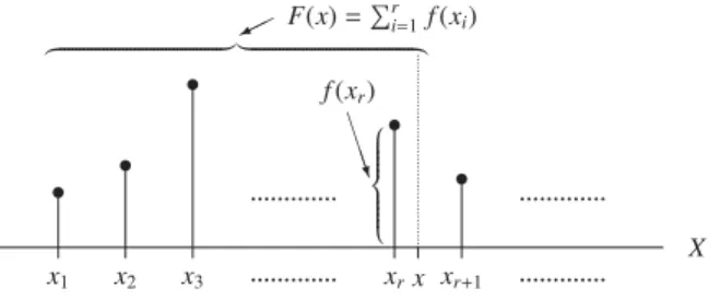
68 1. Discrete random variable (Figure 1):

• F(x) =

r

i=1

f (x

_i

) =

r

i=1

p

_i

,

where r denotes the integer which satisﬁes x

r

≤ x <

x

_r+1

.

• F(x

i

) − F(x

i

− ) = f (x

i

) = p

i

,

where is a small positive number less than x

i

− x

_i−1

.

2. Continuous random variable (Figure 2):

• F(x) =

_x

−∞

f (t) dt,

• F

(x) = f (x).

f (x) and F(x) are displayed in Figure 1 for a discrete random

variable and Figure 2 for a continuous random variable.

(3)

Figure 1: Probability Function f (x) and Distribution Func- tion F(x)— Discrete Case

X

x1 x2 x3 ... xrx xr+1 ...

• •

•

... • ...

⎧⎪⎪⎪⎪⎪⎨

⎪⎪⎪⎪⎪

⎩ BBBN f(xr)

F(x)=r

i=1f(xi)

Note thatris the integer which satisﬁesxr≤x<xr+1.

71 Figure 2: Density Function f (x) and Distribution Function F(x) — Continuous Case

x

X f(x)

@@R F(x)=x

−∞f(t)dt

....

. . . .. . . . . .. .

. .

. ....

....

. ....

..

....

. ....

....

... ....

....

..

....

..

....

.

....

...

....

..

....

.

....

...

....

..

....

.

....

...

....

..

....

...

....

.

....

...

....

..

....

...

....

...

....

...

....

...

....

...

....

..

....

...

....

.

....

...

....

..

....

...

....

.

72

2.2 Multivariate Random Variable (ଟมྔ֬

཰ม਺) and Distribution

We consider two random variables X and Y in this section. It is easy to extend to more than two random variables.

Discrete Random Variables: Suppose that discrete random variables X and Y take x

1

, x

2

, · · · and y

1

, y

2

, · · ·, respec- tively. The probability which event {ω; X(ω) = x

_i

and Y (ω) =

73 y

_j

} occurs is given by:

P(X = x

_i

, Y = y

_j

) = f

_xy

(x

_i

, y

_j

) ,

where f

_xy

(x

_i

, y

_j

) represents the joint probability function (݁߹֬཰ؔ਺) of X and Y. In order for f

_xy

(x

_i

, y

_j

) to be a joint probability function, f

_xy

(x

_i

, y

_j

) has to satisﬁes the following properties:

f

_xy

(x

_i

, y

_j

) ≥ 0 , i , j = 1 , 2 , · · ·

i

j

f

_xy

(x

_i

, y

_j

) = 1.

74 Deﬁne f

_x

(x

_i

) and f

_y

(y

_j

) as:

f

_x

(x

_i

) =

j

f

_xy

(x

_i

, y

_j

), i = 1, 2, · · · , f

y

(y

j

) =

i

f

xy

(x

i

, y

j

), j = 1, 2, · · · .

Then, f

_x

(x

_i

) and f

_y

(y

_j

) are called the marginal probability functions (पล֬཰ؔ਺) of X and Y.

f

_x

(x

_i

) and f

_y

(y

_j

) also have the properties of the probability functions, i.e.,

≥ = ≥ =

Continuous Random Variables: Consider two continuous random variables X and Y. For a domain D, the probability which event {ω; (X(ω), Y (ω)) ∈ D } occurs is given by:

P((X , Y) ∈ D) =

D

f

_xy

(x , y) dx dy ,

where f

_xy

(x , y) is called the joint probability density func-

tion (݁߹֬཰ີ౓ؔ਺) of X and Y or the joint density

function of X and Y.

(4)

f

_xy

(x , y) has to satisfy the following properties:

f

_xy

(x, y) ≥ 0,

_∞

−∞

_∞

−∞

f

_xy

(x , y) dx dy = 1.

Deﬁne f

_x

(x) and f

_y

(y) as:

f

_x

(x) =

_∞

−∞

f

_xy

(x , y) dy , for all x and y, f

_y

(y) =

_∞

−∞

f

_xy

(x , y) dx ,

where f

_x

(x) and f

_y

(y) are called the marginal probability 77

density functions (पล֬཰ີ౓ؔ਺) of X and Y or the marginal density functions (पลີ౓ؔ਺) of X and Y.

For example, consider the event {ω ; a < X( ω ) < b , c <

Y( ω ) < d } , which is a speciﬁc case of the domain D. Then, the probability that we have the event {ω ; a < X( ω ) < b , c <

Y(ω) < d} is written as:

P(a < X < b, c < Y < d) =

_b

a

_d

c

f

xy

(x, y) dx dy.

78 The mixture of discrete and continuous RVs is also possible.

For example, let X be a discrete RV and Y be a continuous RV. X takes x

1

, x

2

, · · ·. The probability which both X takes x

i

and Y takes real numbers within the interval I is given by:

P(X = x

_i

, Y ∈ I) =

I

f

_xy

(x

_i

, y) dy . Then, we have the following properties:

f

_xy

(x

_i

, y) ≥ 0 , for all y and i = 1 , 2 , · · · ,

i

_∞

−∞

f

xy

(x

i

, y) dy = 1.

79 The marginal probability function of X is given by:

f

x

(x

i

) =

_∞

−∞

f

xy

(x

i

, y) dy,

for i = 1, 2, · · ·. The marginal probability density function of Y is:

f

_y

(y) =

i

f

_xy

(x

_i

, y) .

80

2.3 Conditional Distribution

Discrete Random Variable: The conditional probability function (৚݅෇֬཰ؔ਺) of X given Y = y

_j

is represented as:

P(X = x

_i

| Y = y

_j

) = f

_x|y

(x

_i

| y

_j

) = f

_xy

(x

_i

, y

_j

)

f

_y

(y

_j

) = f

_xy

(x

_i

, y

_j

)

i

f

_xy

(x

_i

, y

_j

) . The second equality indicates the deﬁnition of the conditional probability.

The features of the conditional probability function f

_x|y

(x

_i

| y

_j

) are:

f

_x|y

(x

_i

| y

_j

) ≥ 0 , i = 1 , 2 , · · · ,

i

f

_x|y

(x

_i

|y

j

) = 1, for any j.

(5)

Continuous Random Variable: The conditional probability density function (৚݅෇֬཰ີ౓ؔ਺) of X given Y = y (or the conditional density function (৚݅෇ີ౓ؔ

਺) of X given Y = y) is:

f

_x|y

(x|y) = f

_xy

(x, y)

f

_y

(y) = f

_xy

(x, y)

_∞

−∞

f

xy

(x, y) dx .

83 The properties of the conditional probability density function f

_x|y

(x | y) are given by:

f

_x|y

(x | y) ≥ 0 ,

_∞

−∞

f

_x|y

(x | y) dx = 1, for any Y = y.

84 Independence of Random Variables: For discrete random variables X and Y, we say that X is independent (ಠཱ) (or stochastically independent (֬཰తʹಠཱ)) of Y if and only if f

xy

(x

i

, y

j

) = f

x

(x

i

) f

y

(y

j

).

Similarly, for continuous random variables X and Y , we say that X is independent of Y if and only if f

_xy

(x , y) = f

_x

(x) f

_y

(y).

When X and Y are stochastically independent, g(X) and h(Y ) are also stochastically independent, where g(X) and h(Y) are functions of X and Y .

85