Investment Behaviors by Capital Good and Enterprise Size:
Testing Capital Goods Heterogeneity and Capital Market Imperfection with the FSSCI
*Jun-ichi Nakamura
General Manager, Research Institute of Capital Formation, Development Bank of Japan.
Konomi Tonogi
Assistant Professor at the Faculty of Economics, Rissho University.
Kazumi Asako
Professor at the Faculty of Economics, Rissho University, Professor Emeritus in Hitotsubashi University.
Abstract
This paper examines the validity of the Multiple q model, an augmented version of the Tobin’s q theory to consider the heterogeneity of capital goods, using individual firm data which includes small and medium-sized enterprises as well as large ones. We divide capital goods into land and non-land tangible fixed assets, taking into account the imperfection of the capital market, and estimate the Multiple q investment equations by corporate size based on FY 2004-2013 annual survey slips of the Financial Statements Statistics of Corporations by Industry (FSSCI) collected by the Ministry of Finance, Japan.
Our estimation results show that, irrespective of enterprise size, land itself should be treated as an independent capital good that incurs unique adjustment costs as confirmed by earlier studies on publicly listed Japanese firms, indicating the validity of the Multiple q model by considering explicitly the heterogeneity between land and non-land tangible fixed assets. However, at the same time, we find that variables such as debt ratio and tangibility that are considered as redundant under the standard Tobin’s q theory have significant explanatory power and that there are lumpy investment behaviors that cannot be handled by a smooth adjustment cost function presumed for the Tobin’s q theory. Our estimation results also suggest that the lumpiness of investment behaviors is higher for smaller firms and that capital market imperfection would constrain some lumpy investments.
Keywords: capital investment, capital goods heterogeneity, Multiple q, capital market imperfection, lumpy investment
JEL Classification: D22, D92, E22, G31
* This study was supported by JSPS Grant-in-Aid for Scientific Research (B), grant number 25285062 and the FY2015 Joint Use and Research Center Project of the Institute of Economic Research, Hitotsubashi University. We would like to thank the members of the editorial committee who provided valuable advice at the intermediate and final stages of writing this paper. Any remaining errors are the authors’ own. The content of and opinions in this paper are solely attributable to the authors and are unrelated to any organization with which they are affiliated.
I. Introduction
The standard approach to the empirical analysis of corporate investment behavior is the so-called “q theory” or “q model,” in which the investment rate is a linear function of only the “q” ratio, which is the firm’s market value measured by its capital goods (in other words,
“q” becomes a sufficient statistic). With the concept of Tobin (1969) as a starting point, q theory was established with a neoclassical micro-foundation alongside the investment adjustment cost. As is well-known, the explanatory power with regards to actual investment data from estimates of the q theoretic linear investment equation was proved to be unsatisfactory. Due to its theoretical robustness, however, its importance as a benchmark for analysis remains unchanged.
Quite a few research projects have been conducted on the poor empirical applicability of q theory or on improvements to the models based on it. Discussions are still ongoing and can be broadly categorized into two directions. The first is a rethinking of the theoretical assumptions of q theory; the second is an attempt to improve the empirical analysis in terms of the selection of the dataset and techniques for a more refined analysis. In the former research, the real-world validity of assumptions such as single capital goods (or homogeneous multiple capital goods), the quadratic adjustment cost function, and the perfect capital market have been examined, and attempts have been made to explain the broader reality. The latter strand of research includes a search for estimation methods that can overcome measurement errors in the “q” ratio, analyses based on panel data collected from time series data by company or by industry, and the stricter treatment of “negative investments,” such as the disposal and sale of facilities.1
This paper is the first to attempt estimations of the investment function in the Multiple q framework (“Multiple q model” hereafter), introduced by Wildasin (1984) and developed and applied by Asako, Kuninori, Inoue, and Murase (1989, 1997), using survey slip data from the Financial Statements Statistics of Corporations by Industry (FSSCI). Following Asako, Kuninori, Inoue, and Murase (1989, 1997), a series of estimations were conducted on the investment function from the Multiple q model framework using data on Japanese firms by, among others, Tonogi, Nakamura, and Asako (2010), Asako and Tonogi (2010), and Asako, Nakamura, and Tonogi (2016). However, these studies all used data on listed firms. There are advantages to analyzing listed firms, as this enables the use of detailed financial data based on securities reports in the form of panel data pooling time series data for each individual firm;
moreover, the data necessary for the analysis, such as those of capital investment and capital stock for each type of capital goods, can be constructed in a strict way. However, the samples will generally be limited to major enterprises.
In this paper, we explore the room to improve the explanatory power of q theoretic frameworks in aforementioned two directions. Namely, the first is towards the direction of
1 See Asako, Nakamura, and Tonogi (2016) for more detail on these discussion points.
rethinking the theoretical assumptions by explicitly dealing with the diversity and heterogeneity of capital goods that the standard q theory abstracts, and the second is towards the direction of expanding the dataset by including unlisted, smaller firms into our sample.
The latter becomes possible for the first time by using individual survey slip data from the FSSCI. The analysis period was set as 10 years, from fiscal 2004 to fiscal 2013, in order to continue on sequentially from the period covered in Tonogi, Nakamura, and Asako (2010) and Asako and Tonogi (2010). Analyzing this period enables us to see whether changes have occurred in the effects of the heterogeneity of capital goods since fiscal 2004 for the major enterprises.
Much of the research on investment behavior across sample periods has incorporated the possibility that the capital market is imperfect, including studies on small and medium-sized emterprises (SMEs), but all of these studies were based on the assumption of single capital goods. After controlling for the heterogeneity of capital goods, we can expect to obtain new findings on how the imperfect nature of the capital market affects investment behavior by considering how relationships among and the significance of financial variables such as leverage, which should be inherently redundant under the perfect capital markets, differ depending on enterprise size. The FSSCI has fewer survey items than those disclosed in a securities report and is also affected by replacements of the sample firms. Thus, a conventional method of analysis premised on panel data cannot simply be applied. Therefore the techniques developed to construct the dataset with acceptable quality under these constraints is another important contribution of this paper.
The rest of this paper is organized as follows. Section II reviews the framework of Multiple q investment equation. Section III explains the framework of the empirical analysis and data construction. Section IV presents the main results of our estimation for the investment function incorporating capital goods heterogeneity by enterprise size based on the survey slip data from the FSSCI and interprets them. Finally, Section V provides a conclusion and discusses future research possibilities.
II. Investment function from the Multiple q model
Many studies have discussed the theoretical foundations of the Multiple q model and its methods of empirical analysis, starting with Asako, Kuninori, Inoue, and Murase (1989, 1997) and Tonogi, Nakamura, and Asako (2010). Therefore, this section provides only an overview focusing on how the basic form of the investment function used in this paper was derived and the meanings of the concepts used in the analysis.
II-1. Multiple q model
Wildasin (1984) was the first to attempt extending the standard Tobin’s q theory by relaxing the assumption of homogeneous capital goods and followed by Asako, Kuninori, Inoue, and Murase (1989). Wildasin (1984) showed that, in the multiple goods model, a
monotonic one-to-one relationship between the simply totaled investment amount and the
“q” ratio does not hold any longer but that q can be expressed as a linear combination of the investment amount for each of the multiple capital goods.
Asako, Kuninori, Inoue, and Murase (1989) called the multiple goods theory in Wildasin (1984) the “Multiple q theory” and called the conventional q theory that assumes homogeneous capital goods the “Single q theory.” They showed systematically in what sense the Multiple q theory can be regarded as the generalization of Single q theory by introducing new concepts such as “Partial q,” corresponding to the “q” ratio by capital good, and “Total q,” their integration. They also established the fundamental methodology for the empirical analysis, including a statistical test for whether the heterogeneity of capital goods, an assumption of Multiple q theory, is valid. Tonogi, Nakamura, and Asako (2010) noted that, while the correspondence with theory is unclear in the continuous time model, the empirical analysis using financial data requires specifying the timing of capital investment at the beginning or the end of the fiscal period (in other words, whether capital investment in the current fiscal period will contribute to production in the same fiscal period), and they derived two kinds of investment function based on discrete-time models corresponding to each of these two assumptions. They also tested data on Japanese listed firms and confirmed that the “beginning- of-period model” is generally a better fit than the “end-of-period model.”
Based on this beginning-of-period model, Asako and Tonogi (2010) reconstructed concepts such as “Partial q” and “Total q” developed for the continuous-time model in Asako, Kuninori, Inoue, and Murase (1989, 1997) in the context of the discrete-time model.
Moreover, they considered expanding the Multiple q model to ease the assumption of a smooth, convex adjustment cost function. Below, we provide a brief overview of the basic theoretical framework used in this paper for the analysis of the survey slip data of FSSCI̶
the beginning-of-period version of Multiple q model that assumes a smooth, convex adjustment cost function.
In the beginning-of-period model, a firm’s owner–manager makes investment decisions in each period based on information about the businesses environment observed at the beginning of the period (represented by productivity shock A) and immediately carries out the investment. Newly installed capital stock contributes to full production during the current period, and capital depreciation for one period occurs at the end of the period. There are n types of capital goods, and let the physical depreciation rate of j-th capital goods be denoted by δj (j=1,2, ... ,n), the capital stock at the end of the previous period after the depreciation by (1-δj) Kj, the capital investment at the beginning of the current period by Ij, and the capital stock after the investment by K'j. Then, we should have
(1) and the net investment rate Zj after the capital depreciation is written as
(2) which can take any value in the range of Zj≤1/(1-δj), including negative values. When investing, the firm has to incur the adjustment cost, in addition to the purchase costs of capital goods. We assume the adjustment cost can be separated for each capital good and expressed as the quadratic function of the investment rate Zj of the relevant capital good as follows:
(3) The parameter γj>0 represents the size of the adjustment cost (strength of friction) for each capital good, and aj is the parameter corresponding to the investment rate in which the adjustment cost takes the minimum value. The more the investment rate Zj deviates from aj, the greater the rate of increase of the adjustment cost.2
The firm’s production (gross profit) function is assumed to be of a Cobb–Douglas type:
(4) where αj's are nonnegative constants. Then, the Bellman equation of the dynamic optimization problem for the maximization of enterprise value V in each period is expressed as follows:
(5)
Here, pj is the price of capital good j relative to the product price as the numeraire, β is the discount factor, and EA'|A{・} is the expected value operator based on the forecasted productivity shock in the next period, which is based on information on the current period. As both the production function and the investment adjustment cost function are homogeneous of degree one, the value function V also becomes homogeneous of degree one for n capital stocks.
On partially differentiating equation (5) with regards to Kj, the first-order maximization condition for enterprise value is expressed as follows:
2 As with Zj , aj can take any value in the range of aj≤1/(1-δj), including a negative value.
(6)
From Euler’s theorem on homogeneous functions
(7) is established. Thus, from equations (6) and (7),
(8) follows immediately.
Therefore, on dividing both sides of equation (8) by and rearranging it, we obtain the following investment function:
(9)
Here, the three newly defined variables are in order, namely
(10) as the average q by weighted average of the capital goods when aggregating n kinds of capital goods;
(11) as the implicit deflator of the aggregated capital stock;and
(12) as the share of each of the capital goods in the aggregated capital stock.3
3 Here, on placing the constraint that the two adjustment-cost function parameters of γj and γjaj shall be equal for all the capital goods, equation (9) is reduced to the standard investment function (Single q model, where the investment rate is a linear function of the average q) based on the assumption of single capital goods.
Equation (9) is our investment function in the Multiple q model. (q-1)P, Zjsj, and sj
appearing in (9) are all observable data; thus, in accordance with (9), once the term (q-1)P is linearly regressed on the variables Zjsj and sj, we can obtain the estimates of γj and γjaj, which are the coefficient parameters of the adjustment cost function.
As the right side of equation (9) is transformed into
(13)
it is understandable that (q-1)P is equal to the weighted average of the marginal efficiency of each capital good, with the weight as sj.
Asako, Kuninori, Inoue, and Murase (1989, 1997) named the marginal profitability of each capital good divided by the capital-good purchase price, i.e.,
(14) the “Partial q” of that capital good, and named the normal average q “Total q,” in the sense that it is the concept of q that covers all capital goods. From equations (13) and (14), it is understood that the relationship between Total q and Partial q is
(15)
or
(16) And, once the Partial q of (14) is substituted into equation (6), we obtain the relationship between the Partial q and the investment rate Zj defined in (2) as
(17) from which,
(18) is derived. Thus, the investment rate of each capital good is expressed by the linear function of the corresponding Partial q.
II-2. Review of the empirical research on the Multiple q model
As explained, Asako, Kuninori, Inoue, and Murase (1989, 1997), Tonogi, Nakamura, and Asako (2010), and Asako and Tonogi (2010) estimated the Multiple q investment function assuming a smooth, convex adjustment cost function and making use of listed firm data and average q based on share price information. We briefly review the main results obtained from these analyses.
Asako, Kuninori, Inoue, and Murase (1989, 1997), analyzing the manufacturing industry, obtained estimates from two types of capital goods, land and capital stock other than land, as this paper does. Here, the calculation of capital stock other than land followed the method of Hayashi and Inoue (1991). After creating capital stocks and gross investment series for multiple capital goods that considered the differences in the price-change rate and capital deprecation rate for five types of capital assets, such as buildings, structures, and machinery, those were totaled together with inventory. Asako et al. (1989, 1997) focused on land within capital goods and carried out the analysis from two capital goods because, in those days, land in Japan was being actively invested in alongside the rapid increase in the share prices and land prices; it was thought that treating land as a capital good (a quasi-fixed factor of production) that incurs a unique adjustment cost when it is invested in might improve the goodness of fit of the q model.
For this reason, great care was taken in constructing the land data, and precise calculations were made considering elements such as the differences in the rates of increase of land values according to purpose of use and location. Using cross-section data from each year, the validity of the following three models was tested:
Model 1 (Single q that does not include land): There is no adjustment cost for investment in land and thereby Partial q of land is always equal to one.
Model 2 (Single q that includes land): Land is homogeneous with other capital goods and can be added as it is.
Model 3 (Multiple q): There are different adjustment costs for investments in land and for investments in buildings, machinery and equipment; land and other capital goods each has different Partial q.
Asako, Kuninori, Inoue, and Murase (1989), analyzing from fiscal 1977 to fiscal 1987, showed that, within the Single q framework, cases in which land was included in capital stock were more compatible with q theory than were cases in which it was not. In addition, the results of the estimations from the Multiple q model showed clear differences in the estimation values of the adjustment cost parameter of land and capital stock other than land
indicating that the Single q model was not suitable. However, there were some years in which the Partial Q corresponding to pj(qj-1) in equation (18) obtained from the estimation results of the Multiple q model took a negative value. Moreover, although the estimated values for Partial Q of capital stock other than land were somewhat consistent with the trend in the investment rate, inconsistencies with theory remained regarding the results for land; for example, the investment rate for land was consistently positive even in years in which a negative Partial Q was obtained. Asako et al. (1989) argued that the land Partial Q was negative (qj was less than one) because of a bubble in land prices and an excessively high price of land as a capital good.
Asako, Kuninori, Inoue, and Murase (1997), who extended the analysis period up to fiscal 1994 to be sequential with the previous study, tried to answer the questions left unanswered in Asako at al. (1989) by making modifications, such as excluding the increase in the value of land due to increased real land prices from land investment by individual firms as well as using the concept of gross investment rather than net investment for capital goods other than land. As a result, while Asako et al. (1989) found several years in which the Partial Q of capital goods other than land took a negative value, this value became positive every year holding stable and positive correlation with the gross investment rate consistently with the theory. On the other hand, the Partial Q of land, which took a positive value for several years in Asako at al. (1989), was negative every year, and the result was once again inconsistent with the gross investment rate of land. Although land was a factor of production with its own unique adjustment costs, according to their interpretation, this result might have been caused by a bubble in land prices and the overestimation of its contribution as a factor of production.
Subsequently, Tonogi, Nakamura, and Asako (2010) and Asako and Tonogi (2010) analyzed the Multiple q model based on unbalanced panel data from approximately 2,500 listed firms including the non-manufacturing industry, covering from fiscal 1982 to fiscal 2004 (divided into four periods for each business cycle phase). After subdividing capital goods other than land into four categories (i.e., buildings and structures; machinery and equipment; vessels and vehicles; and tools, furniture, and fixtures), they created a time series for gross investment and capital stock using three data construction methods with regard to the evaluation of the sale and the retirement amounts for existing facilities. They also added the cash flow ratio and the interest-bearing debt ratio as additional control variables, and they estimated the Multiple q investment function.
First, Tonogi, Nakamura, and Asako (2010) rejected the null hypothesis that the parameters relating to the adjustment costs of the five types of capital goods, including land, were all equal for all four sample periods. Based on this result, Asako and Tonogi (2010), considering the possibility of partial homogeneity, tested the homogeneity between “certain capital goods” and the “other four capital goods that are regarded (temporarily) as homogeneous,” and also conducted a pairwise test in which any two of the capital goods were homogeneous. They confirmed that, while partial homogeneity was not rejected in some cases, these combinations were not uniform depending on the sample period and the data
construction method regarding gross investment and capital stock, and concluded that the Multiple q model should be used based on the assumption that these five capital goods were fundamentally heterogeneous. However, concerning the goodness of fit as the investment function, the significance and robustness of the parameters of the adjustment cost function were not high. Even in cases with relatively high explanatory power, where the sales and retirement amounts of existing facilities were considered as being uniformly zero, the cash flow ratio and the interest-bearing debt ratio, which should be inherently redundant in the framework of q theory, were estimated to be significant; it was confirmed that factors remained that could not be explained by simply considering the heterogeneity of capital goods while maintaining the same convex-type adjustment cost framework.4
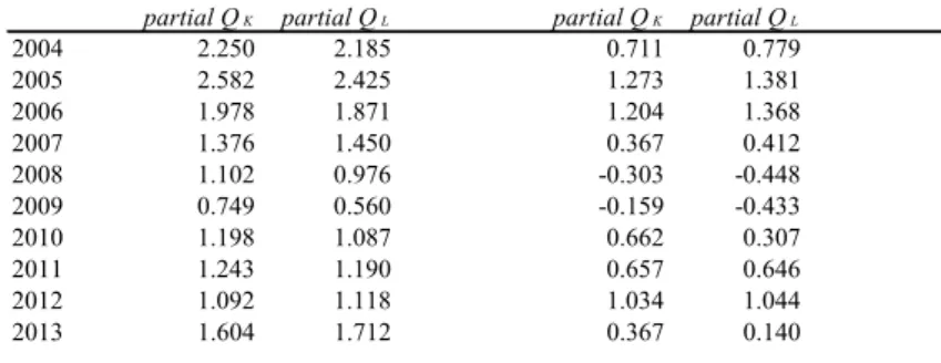
The parameter of the adjustment cost function was often estimated to be insignificant, perhaps due to the influence of additional control variables. There were also major differences in the estimates of Partial q in Asako and Tonogi (2010) depending on the analysis period and the data construction method. In these results, the estimates of land Partial q were comparatively stable, and, regardless of the data construction method, they took significantly positive values in the estimation periods up to bubble economy periods (1982-86, 1987-91) and significantly negative values in the estimation periods after the collapse of a bubble economy (1992-97, 1998-2004).
II-3. Analysis by corporate size using the individual survey slip data from the FSSCI The individual survey slip data from the FSSCI have only two categories of information on tangible fixed assets̶land and capital goods other than land̶and it is difficult to form panel data over a long period of time because the data are collected on a random sampling basis for smaller enterprises. Our dataset also has various restrictions, such as the absence of market evaluations of firm value and the impossibility of using the perpetual inventory method to construct the capital stock data. On the other hand, it targets enterprises of a wide range of sizes, from listed firms to micro enterprises with share capital of less than 10 million yen. Therefore, when conducting estimates from the Multiple q model, it has the advantages described below.
First, one of the reasons why the investment function including Multiple q was not always a good fit in the research on listed firms is that most listed firms have several business units belonging to different industries, and it may be impossible to ascertain their investment behavior with a single function. Moreover, q theory is premised on perfect competition, which may not be even close to reality among listed firms. These problems are less serious for smaller firms. If an investment function that is a poor fit for major enterprises is found to be significant for SMEs, this would seem to support the conjecture described above.
4 From this, Asako and Tonogi (2010) and Asako, Tonogi, and Nakamura (2014) eased the constraint of a smooth, convex adjustment cost function and attempted to estimate the nonlinear Multiple q investment function. Although this line of extension yielded new findings, this paper does not deal with the discussion of non-convexity.
Conversely, an analysis of the investment behavior of manufacturing business establishments in the United States by Doms and Dunne (1998) found that the smaller the establishment, the more pronounced the characteristics of so-called “lumpy investment” behavior. Lumpy investments cannot be analyzed within the framework of the smooth, convex adjustment cost function that is assumed by the Multiple q model in this paper. If this effect is strong, a fit for SMEs would be rather poorer than major enterprises.
Second, by comparing the Single q model and the Multiple q model based on the assumption that the convex adjustment cost function framework has a certain degree of real- world validity, we can test with respect to each firm size whether land is a capital good with an adjustment cost, and, if so, whether there is intrinsic heterogeneity between land and capital stock other than land. For instance, if the land-acquisition behaviors of small enterprises are fundamentally synonymous with the acquisition of new buildings and the expansion of business establishments, land may be homogeneous with capital stock other than land, or otherwise, as small enterprises tend to acquire small parcels of land, the adjustment cost may also remain within a negligible range.
Third, the fact that the cash flow ratio and interest bearing debt ratio are estimated to be significant in the investment function was formerly considered evidence that the imperfect nature of the capital market, such as liquidity constraints, influences investment behavior.
However, the fact that even among listed enterprises, which should be able to easily access the capital market, and even after controlling the simultaneity problems which would cause spurious correlation, these variables are still robustly significant, thus casting doubt on this interpretation. As an alternative explanation, for example, non-negligible measurement errors in the “q” ratio or information on future investment opportunities that cash flow contains have been pointed out though this issue has not yet been settled. To address this point, it would be useful to compare major enterprises and SMEs, which differ in accessibility to the capital market, and to analyze the time period of a global financial crisis in which even major enterprises face liquidity constraints. Although this sort of research has already been carried out to some extent, this paper would seem to be the first that occurs within a framework that includes land investment specific to Japanese enterprises and that takes the heterogeneity of capital goods into consideration.
III. Empirical analysis framework and data construction
As mentioned, individual survey slip data from the FSSCI used for this analysis have various restrictions that differ from those for listed firms. Since it is not possible to simply apply conventional analytical methods that assume panel data based on securities reports, we develop appropriate techniques to deal with the data constraints in the empirical analysis.
III-1. Basic framework of the analysis
In the basic framework for the analysis described below, we estimate the equation which
includes several control variables such as cash flow ratio and interest-bearing debt ratio as well as the year, industry, and other dummy variables into the right-hand-side of equation (9) using the individual survey slip data from FSSCI (for all industries except the financial and insurance industries). There are three major constraints with analyzing FSSCI data compared to previous studies using data on listed firms: (i) it is not possible to calculate the average q using share prices, (ii) it is not possible to construct capital stock data by the perpetual inventory method due to the difficulty in forming panel data, and (iii) there are only two categories of capital goods̶land and goods other than land.
Regarding the first two constraints, we have to find appropriate proxy variable of marginal q which comprises the dependent variable, and also have to construct the capital stock using various techniques, such as borrowing the market to book value ratio and the deflator for each capital good by industry from the listed firms’ data. The rest of this section explains the basic ideas behind the proxy of marginal q. Section III-3 describes the basic ideas behind the construction of the parameters that are necessary for calculating q and the capital stock and investment-related data.
In conventional q theory developed with the assumption of single capital goods, marginal q is defined as “the sum of discounted present value of expected marginal earnings that will be newly created in the future by adding one unit of capital stock in the current period (i.e., the shadow price of capital) divided by the replacement cost of one unit of capital goods.”
When it is problematic to use the average q based on share prices to estimate the investment function, for reasons such as the existence of a share-price bubble, some proxy of marginal q are used instead. For example, if linear homogeneity is assumed with regards to the value function, marginal earnings are equivalent to average earnings; thus, a lot of previous studies estimate the marginal q with vector autoregression (VAR) model using the data of current average return on capital (or profit rate) obtained from the accounting values under the assumption that the stochastic process for the past profit rate and discount rate estimated from the VAR model will be stable over time.5 However, this method cannot be applied here, as panel data cannot be used. Therefore, marginal q is estimated below assuming a steady state in which the static expectation formation becomes a rational expectation formation.
When assuming a steady state, in general two estimation methods can be considered depending on whether or not the capital depreciation rate is included in expected marginal earnings (EME), which is the marginal q numerator. Thus, with ρ as the current period’s profit rate, δ as the depreciation rate, r as the discount rate, and g as the expected growth rate, EME by the net method is expressed as
(19) and by the gross method that considers capital depreciation as
5 See, for example, Abel and Blanchard (1986) and Otaki and Suzuki (1986).
(20) While it is not clear which is the main focus of investors and of enterprises, in the correspondence with the actual data, if any of the denominators or numerators take negative values, the estimates of marginal q implicitly computable from equations (19) to (20) as the ratio EME/K, becomes non-existent and thereby are left out of our sample. Therefore, the gross method is used in this paper to reduce the probability of this non-existence problem occurring.6 For expected growth rate g, we do not find a candidate proxy except for the growth rate of the book value of total assets (BTA) available in our dataset based on the FSSCI. However, it is a rather noisy proxy and the possibility that the denominator takes a negative value in (20) may increase. Taking these shortcomings into account, we uniformly set g as zero for all samples without estimation.
III-2. Control variables and the estimation equation
In addition to the above calculation which is the backbone of the investment function based on Tobin’s q theory, we follow Tonogi, Nakamura, and Asako (2010) and introduce some control variables that are supposed to be redundant in the framework of q theory to look over the validity of q theory and its assumption of a perfect capital market by checking significance of those control variables. In so doing, we at first introduce the following additional variables, which are often employed in estimations of investment function, to the explanatory variables:
Interest-bearing debt ratio=interest-bearing debt (D)/book value of total assets (BTA), Tangibility= total book value of land and other tangible fixed assets (BK) / book value of
total assets (BTA),
Enterprise size=book value of total assets’ logarithmic value, ln (BTA).
Needless to say, the lower limit of the interest-bearing debt ratio is zero; however, there has been a recent increase in zero-leverage firms that have reached this limit, regardless of enterprise size. Therefore, we further add a zero-leverage dummy (ZLD) to our list of explanatory variables to capture this effect. Incidentally, cash flow, which is frequently used in estimations of the investment function, almost always happens to overlap in terms of numerical values with the marginal q numerator in this paper’s dataset. To avoid a development that would improve the model’s explanatory power in appearance (i.e., purely for the technical reason in the data construction), it was decided not to include it in the list of our explanatory variables.
In the Multiple q model investment function (9), if these control variables are estimated to be significant in addition to the theoretically derived q (to be precise, (q-1)P) because, for instance, the capital market is imperfect, the following interpretation is established for their
6 Refer to Suzuki (2001) as an empirical study that adopted the gross method.
signs.
First, concerning the coefficient of the zero-leverage dummy (ZLD) and the interest- bearing debt ratio (D / BTA), if, for example, (i) the supply-side factors in the capital market (i.e., the higher the profit rate, the greater the bank’s willingness to lend), (ii) the disciplinary effects of debt (i.e., the higher the debt rate, the higher the profit rate from the effects of discipline), and (iii) the tax saving effects of debt (i.e., income deduction from interest expenses) are predominant, it is expected that the coefficient of zero-leverage dummy will be significantly negative and the coefficient of interest-bearing debt ratio will be significantly positive. Contrariwise, if, for example, (iv) demand-side factors in the capital market (high debt ratio due to past low profitability with serial correlations in profit rates) and (v) the risk of bankruptcy (i.e., the higher the debt ratio, the higher the discount rate) are predominant, it is expected that the coefficient of zero-leverage dummy will be significantly positive and the coefficient of interest-bearing debt ratio will be significantly negative. In the estimations of the Multiple q model by Tonogi, Nakamura, and Asako (2010), the zero-leverage dummy was not included in the list of control variables and they targeted listed firms and used the average q for q though, the coefficient of interest-bearing debt ratio was robustly positive and significant.
Second, tangibility is used as a proxy variable for pledgeability, which is considered to promote the use of external debt, in research on the determinants of the capital structure. In the Multiple q model investment function, if pledgeability has the effect of easing borrowing constraints, it is expected that the possibility of realizing earnings opportunities increases, from which tangibility becomes positive and significant with regards to q. Conversely, tangibility is given another role to control the effects of intangible assets, which are not considered in our framework. From this aspect, it is expected that the coefficient of tangibility will be negative and significant for the reasons described below.
To clarify the underlying mechanism of this negative effects, we consider a company consisting only of tangible fixed assets including land (K) and intangible fixed assets (R). For simplicity, real values, nominal values, and book values are assumed to be always consistent.
As assumed in our framework, if intangible fixed assets’ Partial qR is always equal to 1, tangible fixed assets’ Partial qK is calculated as follows:
(21) where V denotes firm value. However, if intangible fixed assets should also be considered as capital stock with an adjustment cost (a quasi-fixed factor of production) in reality and therefore qR deviates from 1, the firm value function is expressed as follows
(22) Then, (21) is replaced by
(23) which indicates that qK of (21) deviates from the true Partial qK by a margin of the second term in the right-hand-side of (23), which is positire insofar as qR>1.
Meanwhile, since by definition tangibility=K/(K+R) is negatively correlated with intangible to tangible capital assets ratio R/K, the second term on the right-hand-side of (23) is correlatives negatively with tangibility. Therefore, in summary, the variable tangibility absorbs the upward bias of qK from its true value, rendering the coefficient estimate of tangibility be negative. Therefore, if this negative effect is greater than the tangible fixed assets’ pledgeability effect, the coefficient of tangibility will likely be negative and significant.
Third, enterprise asset size, ln (BTA), is usually a factor reflecting easing borrowing constraints due to effects such as the diversification of the business portfolio. It is thus expected to take a positive sign. Conversely, if enterprise asset size is positively correlated with the company’s degree of maturity (i.e., it is negatively correlated with growth potential), it may take a negative sign.
Last, year dummies, industry dummies, and capital size dummies are considered as dummy variables in the constant term of the estimation equation. The industry dummies are based on FSSCI industry classification table, and the capital size dummies are based on share capital and classified into four categories: 1 billion yen or more (major enterprises), 100 million yen to 1 billion yen (medium-sized enterprises), 10 million yen to 100 million yen (small enterprises), and less than 10 million yen (micro enterprises).
The final investment function (9) is thus estimated with additional control variables as follows:
(24)
where subscripts K and L correspond to capital goods other than land and land, respectively.
III-3. Data construction and elimination of outliers
The investment related data by the category of capital goods and the parameters necessary for calculating the “q” ratio are constructed according to the process described below.
(i) Nominal investment
As in the studies subsequent to Asako, Kuninori, Inoue and Murase (1997), this paper adopts the concept of “gross investment” for the investment rate, which is calculated by
IK= the difference between the beginning and end of the fiscal period in the book value of tangible fixed assets other than land+depreciation expenses,
IL= the difference between the beginning and end of the fiscal period in the book value of land.
In the survey slip of FSSCI, special depreciation expenses are also surveyed. However, they are basically special tax break measures and often not directly deducted from the book value in the accounting treatment. Therefore, it was judged that noise would increase if they were included in the calculation of IK, so they are excluded. Depreciation expenses in the survey slip include those of intangible fixed assets, which should be excluded from depreciation expenses in our model. However, as the breakdown is unknown, these are difficult to estimate. Therefore, we just exclude samples above a certain ratio of intangible fixed assets to tangible fixed assets as outliers.
(ii) Nominal capital stock
As mentioned, it is difficult to construct sufficient panel data to apply the perpetual inventory method from the survey slip data of FSSCI. Therefore, based on listed firms’
financial data, a nominal capital stock series was created by industry for 1977 onwards using the perpetual inventory method, and calculations are made by multiplying the book value of the survey slip data and the industry’s “market value-book value ratio,” which is the industry’s nominal capital stock value divided by the corresponding book value.
(iii) Deflator
For the capital stock deflator, a real capital stock series by industry and by capital goods from 1977 onwards was created based on the listed firms’ financial data using the perpetual inventory method, and calculations were made by dividing this by the nominal capital stock created in (ii). An attempt was made to create a deflator for investment flow using data on listed firms’ real and nominal capital investment though we did not obtain a stable series.
Therefore, we also use the capital stock deflator in place of the deflator for investment flow.
(iv) Capital depreciation rate δ
Capital depreciation rate δ is obtained by multiplying the depreciation rate of capital stock other than land and the weight of capital stock other than land in real capital stock (as it is natural to consider the depreciation rate of land to be zero). The weighted averages of the depreciation rate by capital goods in Hulten and Wykoff (1977, 1981)7 were used for the depreciation rate of capital stock other than land, with the weights of real capital stock by capital good and by industry from 1977 onwards created using the perpetual inventory method based on listed firms’ financial data. When calculating Single q that does not include land, the depreciation rate of capital stock other than land (not multiplied by the weight) is used for δ.
(v) Profit rate ρ
For each firm and for each year, the values from (ordinary profit/loss before depreciation and interest−taxes paid)/nominal capital stock at the beginning of the fiscal period are used.
Taxes paid are calculated by subtracting after-tax profit/loss from pre-tax profit/loss. When calculating the Single q that does not include land, land is excluded from the denominator of
7 Buildings were 0.047, structures 0.0564, machinery and equipment 0.09489, vessels and vehicles 0.1470, and tools, furniture, and fixtures 0.08838.
the nominal capital stock.
(vi) Discount rate r
In the same way, for each firm and for each year, the values obtained from interest paid and others/(interest-bearing debt+the notes receivable discount balance) are used. However, the discount rate of zero-leverage firms is replaced with the minimum value (>0) among the relevant firms in each year, and for values exceeding 20%, Winsorizing processing is carried out with an upper ceiling of 20%.
Some data were considered outliers and eliminated from the target sample. It was considered that some data included errors caused by respondents’ misunderstanding of the question items or mistaken entries; moreover, transcription or input errors may have occurred when the collected questionnaires were processed, and such values were also considered
“outliers.”
Specifically, variables which are considered to need elimination of outliers based on the theoretical/empirical grounds were as follows. First, in the sample of Q=(q-1)P ≧ 10, the contribution of intangible assets to enterprise value was too great, which is difficult to explain within the framework of this paper; second, the (q-1)P≦−10 sample was meaningless, as it included a proxy variable of q that should theoretically be positive; third, the (depreciation expenses/the book value of depreciable assets)≧1 sample likely included mistaken entries, such as in the entries of the accumulated depreciation amount in current depreciation expenses; fourth, regarding the book value of total assets, the sample showing a large discontinuity such that (end of fiscal period/beginning of fiscal period) ≧ 1.5 was likely due to mergers and acquisitions rather than ordinary economic activities; therefore, these were excluded from the estimations.
III-4. Descriptive statistics
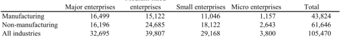
As is summarized in Table 1, a total of 105,470 samples were obtained after the outlier processing for the 10-year period from fiscal 2004 to fiscal 2013. Medium-sized enterprises (with capital of 100 million yen to 1 billion yen) accounted for the greatest portion while major enterprises (with capital of 1 billion yen and above) and small enterprises (with capital of 10 million yen to 100 million yen) were the close second and third. There were 3,800 micro enterprises (with capital of less than 10 million yen), less than 4% of the total. In terms
Table 1. Number of samples by capital size and industry (FY 2004 to 2013)
Table 1 Number of samples by capital size and industry (FY 2004 to 2013) Major enterprises Mediumsized
enterprises Small enterprises Micro enterprises Total
Manufacturing 16,499 15,122 11,046 1,157 43,824
Nonmanufacturing 16,196 24,685 18,122 2,643 61,646
All industries 32,695 39,807 29,168 3,800 105,470
Note: Major enterprises have capital of 1 billion yen and above, mediumsized enterprises have capital of 100 million yen to 1 billion yen, small enterprises have capital of 10 million yen to 100 million yen, and micro enterprises have capital of less than 10 million yen.
of industry, around 40% of firms were from the manufacturing industry, and around 60%
were from the non-manufacturing industry. The manufacturing percentage increased as the size of the firm’s share capital grew and exceeded 50% for major enterprises.
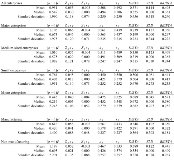
Table 2 shows the basic descriptive statistics of variables for the regression equation of the Multiple q model (24); namely, of (q-1)P as the dependent variable; of ZKsK and ZLsL as the product of the investment rate and the share of capital stock with regards to tangible fixed assets other than land and land, respectively; and of sK and sL as the shares of capital stock with regards to tangible fixed assets other than land and land, respectively; and of the main control variables.
To begin with, the average value of dependent variable (q-1)P is 0.95 and the median value is 0.55 for the whole sample, which seem plausible. These values grew as capital increased. At an industry level, the manufacturing industry average was 0.62, the non- manufacturing industry average was 1.19, nearly twice as high. The average value of ZK sK as the product of the investment rate in fixed assets other than land and the corresponding share
Table 2. Summary statistics by capital size and industry (FY 2004 to 2013)
Table 2 Summary statistics by capital size and industry (FY 2004 to 2013)
All enterprises (q-1)P ZKsK ZLsL sK sL D/BTA ZLD BK/BTA
Mean 0.951 0.055 0.003 0.508 0.492 0.371 0.114 0.405
Median 0.547 0.030 0.000 0.494 0.506 0.325 0.000 0.361
Standard deviation 1.990 0.118 0.074 0.250 0.250 0.456 0.318 0.240
Major enterprises (q-1)P ZKsK ZLsL sK sL D/BTA ZLD BK/BTA
Mean 1.105 0.066 0.004 0.561 0.439 0.239 0.137 0.350
Median 0.673 0.046 0.000 0.563 0.437 0.199 0.000 0.297
Standard deviation 1.975 0.120 0.071 0.235 0.235 0.223 0.344 0.222 Mediumsized enterprises (q-1)P ZKsK ZLsL sK sL D/BTA ZLD BK/BTA
Mean 1.010 0.055 0.004 0.511 0.489 0.350 0.125 0.409
Median 0.575 0.029 0.000 0.491 0.509 0.319 0.000 0.363
Standard deviation 1.988 0.121 0.078 0.247 0.247 0.315 0.330 0.244
Small enterprises (q-1)P ZKsK ZLsL sK sL D/BTA ZLD BK/BTA
Mean 0.764 0.045 0.000 0.450 0.550 0.506 0.081 0.441
Median 0.403 0.017 0.000 0.421 0.579 0.504 0.000 0.413
Standard deviation 1.951 0.110 0.073 0.252 0.252 0.670 0.273 0.235
Micro enterprises (q-1)P ZKsK ZLsL sK sL D/BTA ZLD BK/BTA
Mean 0.445 0.040 0.004 0.475 0.525 0.689 0.045 0.571
Median 0.219 0.005 0.000 0.452 0.548 0.672 0.000 0.580
Standard deviation 2.245 0.106 0.052 0.279 0.279 0.682 0.207 0.252
Manufacturing (q-1)P ZKsK ZLsL sK sL D/BTA ZLD BK/BTA
Mean 0.616 0.058 0.002 0.567 0.433 0.346 0.102 0.350
Median 0.420 0.041 0.000 0.578 0.422 0.291 0.000 0.322
Standard deviation 1.400 0.088 0.048 0.227 0.227 0.564 0.302 0.181
Nonmanufacturing (q-1)P ZKsK ZLsL sK sL D/BTA ZLD BK/BTA
Mean 1.189 0.052 0.003 0.467 0.533 0.389 0.122 0.445
Median 0.693 0.021 0.000 0.426 0.574 0.354 0.000 0.409
Standard deviation 2.291 0.135 0.088 0.257 0.257 0.358 0.328 0.267
of capital stock was 0.055, whereas the average value of ZLsL as the product of the investment rate in land and the corresponding share of capital stock was slightly negative overall. Since the share value is always positive, we understand that the investment rate in tangible fixed assets other than land is correspondingly positive on average, whereas the investment rate in land is negative on average.
The overall average values of sK, sL as the share of capital stock of tangible fixed assets other than land and land are basically half and half. For major and medium-sized enterprises and manufacturing firms, sK is more than half, whereas for small enterprises and micro enterprises and non-manufacturing firms, sL is more than half. The interest-bearing debt ratio (D/BTA) grew as capital decreased; it was 0.24 for major enterprises and reached 0.69 for micro enterprises. It was slightly higher in the non-manufacturing industry. The ratio of zero-leverage enterprises (ZLD=1) was 11.4%, which decreased as capital decreased. It was found that 4.5% of micro enterprises were zero-leveraged. It was slightly higher in the non- manufacturing industry. Tangibility grew as capital decreased, and it was higher in the non- manufacturing industry.
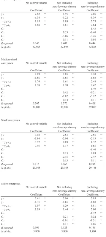
IV. Main estimation results and interpretation IV-1. Baseline model for all sample enterprises
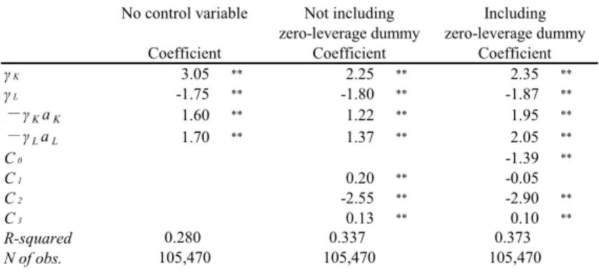
In estimating equation (24), Multiple q model investment function, we run three types of regressions as baseline model depending on the included control variables; namely, with none of the control variables or the case of “no control variable”; with all of the control variables but the zero-leverage dummy or the case of “not including zero-leverage dummy”;
and with all of the control variables or the case of “including zero-leverage dummy”. Table 3 shows the results of the standard OLS (ordinary least squares) estimations for these baseline
Table 3. Baseline model results (FY 2004 to 2013)
Table 3 Baseline model results (FY 2004 to 2013)
γK 3.05 ** 2.25 ** 2.35 **
γL 1.75 ** 1.80 ** 1.87 **
-γKaK 1.60 ** 1.22 ** 1.95 **
-γLaL 1.70 ** 1.37 ** 2.05 **
C0 1.39 **
C1 0.20 ** 0.05
C2 2.55 ** 2.90 **
C3 0.13 ** 0.10 **
Rsquared N of obs.
Note 1. Standard errors are heteroscedastically robust (Huber–White estimator), with ** and * denoting significance at the 5% and 10% levels, respectively.
2. The results of the year dummies, industry dummies, and capital size dummies are omitted from the table.
Coefficient
No control variable Not including
zeroleverage dummy Including zeroleverage dummy Coefficient Coefficient
0.280
105,470 0.337
105,470 0.373
105,470
models.
First, concerning the estimates of γK, γL, -γKaK, -γLaL for three types of regressions, each γ parameter of the tangible fixed assets other than land is significantly positive, while each γ parameter of the land is significantly negative. The fact that parameter γK is positive indicates that the investment behavior for tangible fixed assets other than land does not necessarily contradict the convex, smooth adjustment cost framework. However, the fact that the control variables are also significant in cases of estimation including these variables is not consistent with q theory. The fact that parameter γL is negative is in line with the result obtained in Asako, Kuninori, Inoue, and Murase (1989, 1997) but inconsistent with the result in Tonogi, Nakamura, and Asako (2010).
Tonogi, Nakamura, and Asako (2010) used a more detailed classification for capital goods other than land, but it is unlikely that this affects the results of the land estimates. It is more likely partly attributable to their use of panel analysis controlling firm fixed effects.
Meanwhile, all of the estimation values of -γKaK and -γLaL are positive and significant, suggesting that the investment rate a that minimizes the adjustment cost (3) is negative for tangible fixed assets other than land and positive for land.
Regarding the control variable, C1, the coefficient of the interest-bearing debt ratio, is estimated to be positive and significant if it does not include the zero-leverage dummy, suggesting the possible involvement of supply factors of the lending market, the disciplinary effects of debt, and tax-saving effects; this result is consistent with Tonogi, Nakamura, and Asako (2010). On adding the zero-leverage dummy to the explanatory variables, the coefficient of the zero-leverage dummy C0 is negative and significant, and the interest- bearing debt ratio loses its explanatory power. The results still suggest the involvement of supply factors of the lending market, the disciplinary effects of debt, and tax-saving effects, but many of the positive effects of the interest-bearing debt ratio prove to be attributable to the differences between zero-leverage enterprises and enterprises with debt.
The results of the estimations of the tangibility coefficient C2 and the enterprise asset size coefficient C3 are stable both with and without the zero-leverage dummy, with the former being negative and significant and the latter being positive and significant. The fact that tangibility is negative and significant suggests that the role played by the correction of the distortion of q from the existence of intangible assets is stronger than are the effects of pledgeability. On the other hand, the fact that enterprise asset size is positive and significant may reflect the easing of borrowing constraints from the effects of corporate size.
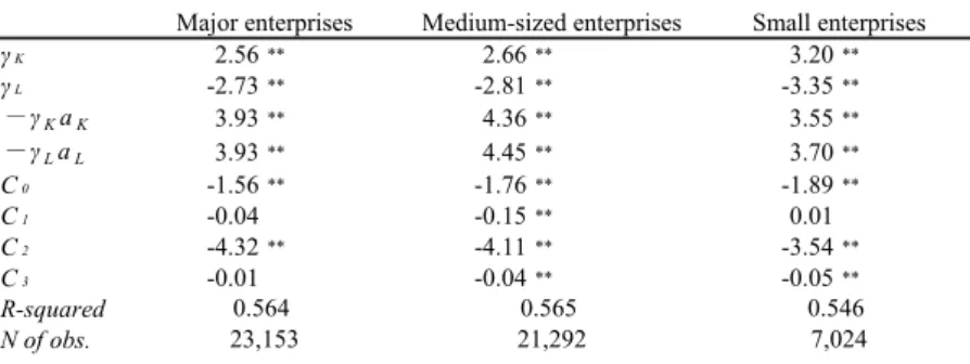
IV-2. Test of the heterogeneity of capital goods: comparison with the Single q model Following Asako, Kuninori, Inoue, and Murase (1989, 1997), this section tests the heterogeneity of capital goods by conducting estimations from three models̶Single q that does not include land, Single q that includes land, and Multiple q̶and by comparing and contrasting their respective performances. When all capital goods are homogeneous, the expression of Multiple q model (9) reduces to