VISUALISATION OF STABILITY REGIONS FOR LOGISTIC DIFFERENCE EQUATIONS WITH MULTIPLE DELAYS (Theory of Biomathematics and Its Applications XI)

YUKIHIKONAKATA,NAOYUKIYATSUDA,ANDEMIKO ISHIWATA

ABSTRACT. We considerlinearisedstability of nonlinear differenceequationsby investi-gatinglocation ofrootsof theassociated characteristicequations.Thecharacteristic

equa-tion is givenas apolynomialequationwith the order determinedby the delayin the dif-ference equation. Forsomepolynomialequationswevisualiseallthe sets ofcoefficients

suchthat allthe rootslocate inside the unit circle in the complex plane. The information

canbetranslatedtounderstand stability of the nonlinear difference equation intermsofits

original parameters. We presentsomeexamples that delay in thedifferenceequationcan

stabilise the equilibrium of theequation.

1. INTRODUCTION: DELAY INDIFFERENCEEQUATIONS

Let$f$be

a

mapping from$\mathbb{R}$to$\mathbb{R}$

.

Inthe

paper

[12] the authors consider

a

difference

equation with

one

single delayin

a

form

(1.1) $x_{n+1}=x_{n}f(x_{n-k}) , n\in \mathbb{N}+,$

where$k\geq 1$ is

a

positiveinteger. initial conditions

are

given

as a

sequence $(x_{0},x_{-1}, \ldots,x_{-k})=(p_{0},p_{1}\ldots,p_{k})\in \mathbb{R}^{k+1}.$

One

can

then compute$x_{1}=p_{0}f(p_{k})$ and recursively construct the solution (as long

as

thesolution exists in the domain of$f$). Theequilibriumof(1.1) is given

as a

rootof the equation

$1=f(x)$

.

Wedenote theequilibriumby$x^{*}$ assuming that itexists. If_$f$is

a

differentiablefunction(at

leastaroundtheequilibrium),

one

can

linearise equation(1.1)aroundtheequilibrium$x^{*}$ to

get

a

linear difference equation:

(1.2) $y_{n+1}=f(x^{*})y_{n}+x^{*}f’(x^{*})y_{n-k}=y_{n}+x^{*}f’(x^{*})y_{n-k}.$

Thelinearisedequation (1.2)leads to thefollowing characteristic equation:

(1.3) $\lambda^{k+1}=\lambda^{k}+x^{*}f’(x^{*})$,

which is

a

polynomial equation ofthe $(k+1)$-thorder. It is known that the equilibrium isasymptotically stable if all therootsof the equation(1.3)locate inside theunitcircle in thecomplex plane(i.e., all the

zeros

of(1.3)havetheirmagnitude less thanone). Werefer

[6, 10]

as

general references forthestability theory of difference equations. Tobeconcrete, let

us

set

$f(x)=\exp\{r(1-x)\}, x\in \mathbb{R}+,$

where$r>0$

.

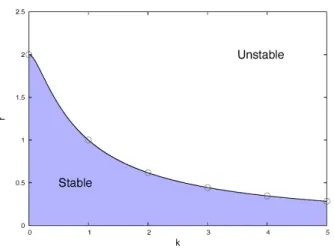
Then equation(1.1)becomes the logistic equation

FIGURE 1.1. Stability region fortheequilibrium of(1.4). Astable equi-librium

can

become unstable

as

$k$

increases.

We refer[10, 12,2]_{for the biologicalmotivationfor thedifferenceequation}(1.4). One

can

easily

see

that theequation (1.4)has the equilibrium

$x^{*}=1$

andthatlinearisationleadstothefollowing characteristic equation:

$\lambda^{k+1}=\lambda^{k}-r.$

In [12]it isshown that theequilibriumisasymptotically stableif

$r<2 \cos\frac{k\pi}{(2k+1)}$

anditis unstable if the

converse

inequality holds. Since the stable equilibrium becomes unstable

as

theparameterof delay$k$increases,

see

Figure 1.1, the resultderives_clich\’e

that delayednegative feedback induces instability.

Does the delayalwaysdestabilise difference equations? Let

us

consider the following differenceequation

(1.5) $x_{n+1}=x_{n}\exp[r\{1-\alpha x_{n}-(1-\alpha)x_{n-1}\}],$

where $\alpha\in[0$,1$]$

.

Stabilityof theequilibrium of(1.5)

was

studiedin [14, 2]. Here,

using

(1.5)

as an

example,

we

would hketoillustrate

our

approachfor stability analysis of

non-linear difference equation. Step oftheanalysis is analoguetothe

one

proposedin [4, 3],

where theauthorsstudy transcendental equations which

are

derived fromcontinuousdelay equations describing population dynamics.

For(1.5) _{the characteristic equation, associated to theequilibrium}$x^{*}=1$_, becomes

a

quadratic polynomial equation:

(1.6) $\lambda^{2}+a\lambda+b=0$

where

(1.7a) $a=r\alpha-1,$

to thecontinuity oftherootswith respect to thecoefficients $(a,b)$

.

One

can

immediately

see

that if

(1.8) $1+a+b=0$

holds,thenequation(1.6)has

a

root$\lambda=1$whileif

(1.9) $1-a+b=0$

holds, then(1.6) has

a

root $\lambda=-1$

.

Those conditions

can

be visualised

as

two lines in the $(a,b)$_-parameterplane that form

a

partof stabilityboundariesin the $(a,b)$_-parameter

plane,

see

Figure 1.2(a).

Equation (1.6) of

course

could have

a

conjugate pair ofcomplexroots with $|\lambda|=1.$ Suppose that$\lambda=e^{i\omega}=\cos\omega+i\sin\omega,$ $\omega\in(0, \pi)$ solves equation(1.6). We getthe

fol-lowingtwoequations

(1.10a) $0=\cos 2\omega+a\cos\omega+b,$

(1.10b) $0=\sin 2\omega+a\sin\omega.$

Theseequations(1.10)

can

be easily solved withrespect to $(a,b)$

as

(1.11) $(\begin{array}{l}ab\end{array})=(\begin{array}{l}-2cos\omega 1\end{array}), \omega\in(0, \pi)$

.

Theequality(1.11)definesaparametriclineby$\omega$inthe$(a,b)$-plane, which

one

can

easily

plot. Alongtheparametricline givenby (1.11),thecharacteristic equation(1.6)has

a

root $\lambda=e^{i\omega}$

(andalso$\lambda=e^{-j\omega}$_), see againFigure 1.2_(a).

Now the $(a,b)$-parameter planeisdecomposedinto

some

regionsby those threelines, wherethe characteristic

equation

(1.6) has

a

rootwith $|\lambda|=1$

.

Todetermne the stability

region, ineachpoint in the$(a,b)$_{-parameter plane,}

one

shouldcount the numberofroots that locate inside/outside_{the unitcircle in} $\mathbb{C}$

.

In general this

can

be done by applying

Rouch\’e’s theorem

as

in [5]. Forequation (1.6), however,

one can

easily verify that the number locating outside theunitcircle in$\mathbb{C}$

as

in Figure 1.2(a)byelementary calculations.

See also Theorem 1.$3.4in$_Chapter1 in[10]for

an

explicit stability condition derived in

a

differentwayapplying the

Schur-Cohn

criterion.

Finally let

us

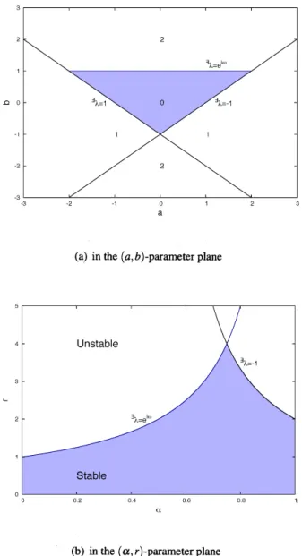
interpret the stability region depictedin Figure 1.2 (a) in terms ofthe

original parameters $(r, \alpha)$ in (1.5). Accordingto (1.7)one canseethat (1.8) amounts to

that$r=0$holds,where thecharacteristic equationhas

a

root$\lambda=1$_,andthat_(1.9)amounts

to

$r= \frac{2}{2\alpha-1},$

where thecharacteristic equationhas

a

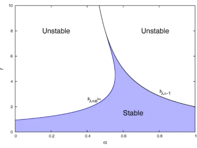
root$\lambda=-1$

.

Theinverse mapping of_(1.7)is

$r=a+b+1,$

$\alpha=\underline{a+1}$ $a+b+1^{\cdot}$

$D$ $O$

$33$

$0$

$a$

(a) in the$(a,b)$_{-parameterplane}

$0$

$0$ 02 04 06 os

(b) in the$(\alpha,r)$-parameterplane

FIGURE 1.2. Stabilityregion for the characteristic equation(1.4).In(a)

thenumber ofrootsthat locateoutsidetheunitcirclein$\mathbb{C}$isdepicted.

Thenoneobtainsthefollowing

curve

correspondingto(1.11)

$(\begin{array}{l}r\alpha\end{array})=(\begin{array}{ll}2-2c\circ s \omega\frac{1-2cos\omega}{2-2cos\omega} \end{array}), \omega\in(0, \pi)$,

which

can

be explicitlyexpressed

as

$r= \frac{1}{1-\alpha}.$

Therefore

as

in Figure1.2(b)

we

can

deduce the stability region forthepositive equilibrium of(1.5) inthe $(r, \alpha)$-parameterplane. Figure 1.2 (b) shows that stability threshold for $r$

In this section

we

would like

Ourmotivation

comes

from stability analysis of the logisticequationwith multiple delays: (2.1) $x_{n+1}=x_{n}\exp[r\{1-\alpha x_{n}-\beta x_{n-j}-(1-\alpha-\beta)x_{n-k}\}],$

where

$r>0, \alpha\geq 0, \beta\geq 0, \alpha+\beta\leq 1$

and$k$and$j$

are

integers such that$k>j.$

Onecaneasily

see

thatequation (2.1)has thepositive equilibrium$x^{*}=1$

.

The

charac-teristic equationfor thepositiveequilibrium$x^{*}=1$ iscomputed

as

(2.2) $\lambda^{k+1}+a\lambda^{k}+b\lambda^{k-j}+c=0,$ where

(2.3a) $a=r\alpha-1,$

(2.3b) $b=r\beta,$

(2.3c) $c=r(1-\alpha-\beta)$

.

To

see

if all therootsof thepolynomial equation(2.2)lieinside theunitcirclein$\mathbb{C}$

,

one

could apply the Schur-Cohn criterion [10]. The direct applicationhowever

may

require

lengthycalculationstoobtainconcreteconditions intermsofparameters,whichwould be ofinterestin thecontextof applicationstobiologicalmodels.

Thecharacteristic equation (2.2)has aquite general form including cases previously studiedinthe literature. For example, (2.2)with $b=0$$(or c=0)$is studied in the famous

paper

[11]. Recently, in the

paper

[1] the authors formulated

an

explicit stability

condi-tionfor(2.2)with $j=k-1$, applyingtheSchur-Cohn

criterion.

Proving contractivity of

the solution for the nonlinear equation (2.1) involves

a

lot ofcomputations and derives sufficient conditions fortheglobal stability of the equilibrium,

see

[13, 16, 15].

Consider thepolynomial equation(2.2) inthe $(a,b,c)$-coefficientspace (insteadof the

plane as in Section 1). We make drastic simplification by assuming that $j=1$ holds,

whichavoids technical detail but shows interesting stability boundaries. Our firstaimisto

characterise the region

$D:=$

{

$(a,b,c)\in \mathbb{R}^{3}$

:

Every root of(2.2)locates inside theunitcirclein$\mathbb{C}$

}.

Define

$L_{1}$ $:=$

{

$(a,b,c)\in \mathbb{R}^{3}$ : (2.2)has aroot$\lambda=1$

},

$L_{-1}$ $:=$

{

$(a,b,c)\in \mathbb{R}^{3}$

:

(2.2)has

a

root$\lambda=-1$

}.

One

can

immediately

see

that$L_{1}$ and$L_{-1}$ respectivelyformplanes:

$L_{1}=\{(a,b,c)\in \mathbb{R}^{3}:1+a+b+c=0\},$

$L_{-1}=\{(a,b,c)\in \mathbb{R}^{3}$

:

$(-1)^{k+1}+a(-1)^{k}+b(-1)^{k-1}+c=0\}.$

We

are

nowinterested in

$C:=$

{

$(a,b,c)\in \mathbb{R}^{3}$ :_(2.2)has

a

conjugate pair of complexrootswith $|\lambda|=1$

Now let

us

introduce

a

sufficient condition for that

every

root locate “outside” the unit circlein$\mathbb{C}$

,i.e.,

no

rootsin insidetheunit circle in$\mathbb{C}$

.

Thefollowing result

can

be easily

provenbyusingthe

fundamental

theorem of algebra. Weomitthe proof.

Lemma

1.

Letus

assume

$that|c|\geq 1$ holds. Then_equation (2.2)hasarootwith $|\lambda|\geq 1$

for

any$(a, b)\in \mathbb{R}^{2}.$

Thus, tofind the stability region,

we

can

restrict

our

attentionto$c\in(-1,1)$

.

_We

intro-ducethefollowingresult.

Theorem2. Equation(2.2)hasaconjugatepair

_of

complexroots$\lambda=e^{\pm i\omega},$ _{$\omega\in(0, \pi)$}

if

andonly

_if

(2.4) $(\begin{array}{l}ab\end{array})=-\frac{1}{\sin\omega}(-c\sin((k-1)\omega)+\sin(2\omega)c\sin(k\omega)-\sin\omega) , \omega\in(0, \pi)$

holds.

Proof

Letussubstitute$\lambda=e^{i\omega},$ $\omega\in(0, \pi)$ into_(2.2). Wethen_get

$0=\cos((k+1)\omega)+a\cos(k\omega)+b\cos((k-1)\omega)+c,$

$0=\sin((k+1)\omega)+a\sin(k\omega)+b\sin((k-1)\omega)$.

Then

one can

getthe conclusion by solvingthe twoequations withrespectto$a$and$b.$ $\square$

Then

we

haveingredientstoplot the stability boundary for given$k$

.

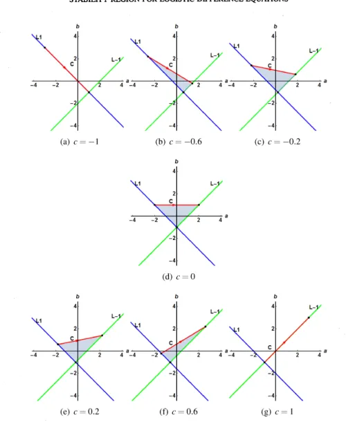
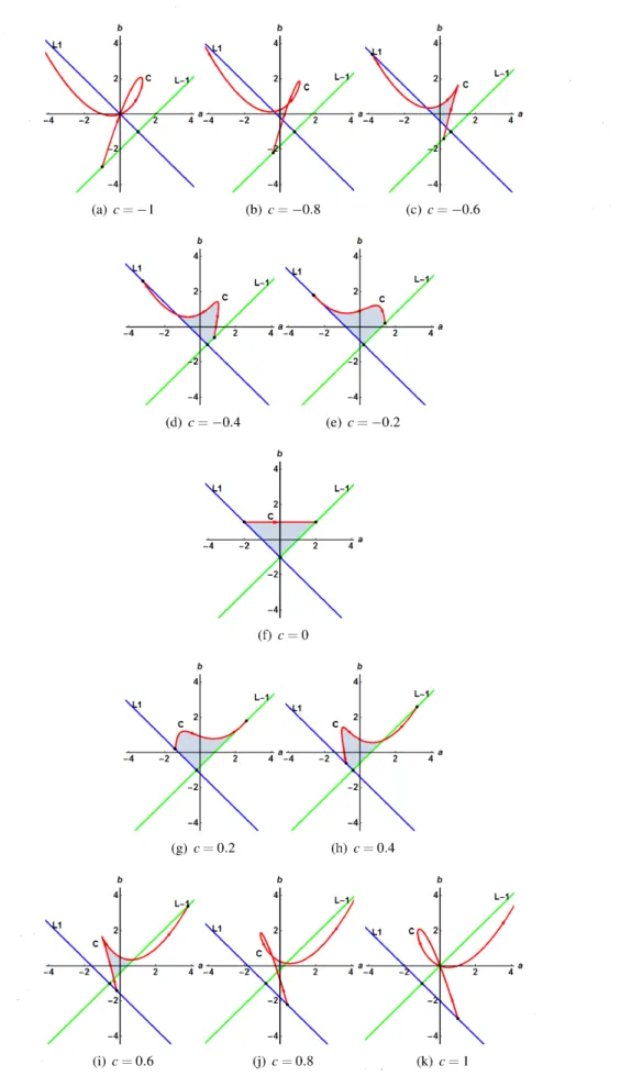
We_present$L_{1},$ $L_{-1}$

and $C$ for several _{$c\in[-1, 1]$ fixing} $k$,

see

Figure 2.1 where_$k=2$ andFigure

2.2 where

$k=4$

.

The colored region is the exact stability region, which

can

be detected by the

application of theRouch\’e’s theorem (we omit the detail,

see

again [5, 3] for the

use

of

theRouch\’e’s theoremtodetermine the stabilityregion). InbothFigures2.1 and2.2

one

can

see

that the stabilityregion disappears

as

$c$becomes $\pm 1$_,

cf. Lemma 1. When$k=4,$ thecharacteristicequation has degree 5and the stabilityboundaryintersectsitself,

see

the

case

that$c=\pm 0.8$ _{holds. The stability boundary thatintersectsitself}

_seems

_tobe

_one

_of

theinterestingproperties of the differenceequation withtwo delays, cf. [9].

_One

could

of

course

visualise the stability region in the $(a,b,c)$-space

as a

_{three-dimensionalobject,}

which could also beinformativetoobserve the fullstructureof the stability region. What

can

we

now

say about stability of the equation (2.1)? To

answer

the question

we

interpretthe obtained stabilityregion inthe$(a,b,c)$-space using_themapping(2.3)_and

formthestability regionintheoriginalparameter space: $(r, \alpha,\beta)$

.

Herewedo notgivea

detailed analysis, but

we

would liketoshow that the stability threshold for$r$

can

be larger

than the

one

obtainedfor theequation(2.1)in Section 1.

Let$k=2$and

we

simphfy the equation(2.1)byassumingthat

$\beta=\frac{3}{4}(1-\alpha)$

holds. Now equation(2.1)hastwo parameters: $(r, \alpha)$

.

Themapping(2.3)becomes

(2.5a) $a=r\alpha-1,$

(2.5b) $b= \frac{3}{4}r(1-\alpha)$, (2.5c) $c= \frac{1}{4}r(1-\alpha)$

.

(d)$c=0$

FIGURE 2.1. Stability region for the characteristic equation (2.2) with

$k=2.$

Corollary

3.

Equation(2.2) has

a

conjugate pair

_of

complexroots $\lambda=e^{\pm i\omega},$ _{$\omega\in(0, \pi)$}

if

and only

_if

(2.6) $(\begin{array}{l}r\alpha\end{array})=(1-\frac{4^{1-}}{3+2c\circ s\omega}(1-2\cos\frac{\omega_{5}}{3+2\cos\omega})^{-1}2\cos\omega+\frac{5}{3+2cos,\omega+}) , \omega\in(0, \pi)$

holds.

Proof

For$k=2$_theset$C$

can

berepresented by

$(\begin{array}{l}ab\end{array})=(\begin{array}{l}c-2cos\omega-2ccos\omega+1\end{array}) \omega\in(0, \pi)$

.

Using(2.5)

_one

has

FIGURE 2.2. Stabilityregion for thecharacteristic equation(2.2) with $k=4$

.

_When$c=\pm 0.8$_the

curve

_{thatrepresents}$C$intersectsitself.

$0_{0} 02 04 06 08$

FIGURE 2.3. Stabilityregionfor the equilibrium of(2.1) in the $(\alpha,r)-$

parameterplane. Two

curves

meet atthepoint $( \frac{1}{2},8)$

.

We

now

solve thetwoequations withrespect to$r$and $\alpha$

.

From the secondequation

we

get

$r(1- \alpha)=\frac{1}{\frac{3}{4}+z^{\cos\omega}1}=\frac{4}{3+2\cos\omega}rightarrow r\alpha=r-\frac{4}{3+2\cos\omega}.$

From the first equation it follows

$r \alpha=\frac{4}{5}+\frac{1}{5}r-\frac{8}{5}\cos\omega.$

From those equations

one

obtain the expression for $r$

as

in (2.6). Then

one can

get the

expressionfor$\alpha.$

$\square$

It

can

beeasily

seen

thatequation(2.2)has

a

root$\lambda=-1$ _when

$r= \frac{4}{3\alpha-1}.$

InFigure2.3

we

plotthose

curves.

One

can

compute that the parametric

curve

given by

(2.6) starts $at$ thepoint $(0,4/(2+\sqrt{5}))$ and ends atthe point $( \frac{1}{2},8)$

.

From the shape

ofthe

curve

one

can

increase $r$

so

that

a

stable equilibriumbecomes unstable and then

again becomes stable, for

some

$\alpha(<\frac{1}{2})$

.

As in Figure

1.2

(b)

an

unstable equilibrium

can

become stable

as

$\alpha$ decreases from 1 to around

0.6

(if$r$ is less than 8). The shape

of the stability boundary shows that delayinthenonlineardifferenceequationindeed.can

contributeto stability of the equilibrium, differently from what

one

could expect in the difference equation with

one

singledelayin Section 1.

Acknowledgement. Thispaper

was

written during the first author’s stayattheBolyai

In-stitute ofthe University of Szeged inJanuary 2015. The first author thanksRobert Vajda for stimulus discussion forcharacterisation of the stability boundary, which will be

pre-sented elsewhere. The first author is grateful toYoshiaki Muroyaforintroductionofthe

research

area.

$YN$

was

supportedby byJSPSFellows,No.268448ofJapanSociety for the

REFERENCES

[1] J. \v{C}erm\’ak, J. Jdnsk\’y,P. Kundr\’at, On necessaryandsufficient conditions forthe asymptotlcstability of higher orderlinear differenceequations, J. Diff. Eq. Appl.,18(2012)1781-1800

[2] E.E.Crone,_{Delayed density dependence and the stability of interacting populations and sub-populations,} Theo. Pop.Bio.,51(1997)67-76

[3] O.Diekmann,Ph.Getto,y.Nakata,On the characteristic equation$\lambda=\alpha_{1}+(\alpha_{2}+\alpha_{3}\lambda)e^{-\lambda}$_{and its}use_in

the context ofacellpopulationmodel(submitted)

[4] O.Diekmann,K.Korvasova,Adidacticalnoteonthe advantageof using twoparametersin Hopfbifurcation

studies, J. Biol. Dyn.7Supplement1(2013)21-30

[5] O.Diekmann,S.A.vanGils,S.M.V.Lunel,H.O. Walther, Delay EquationsFunctional,Complex and Non-linear Analysis, Springer Verlag(1995)

[6] S.N. Elaydi, An IntroductiontoDifferenceEquations.ThirdEdition,Undergraduate Texts inMathematics, Springer(2005)

[7] M.M. Kipnis, D.A.Komissarova, A noteonexplicit stability conditions for autonomous higherorder dif-ference equations, J.Diff. Eq.Appl. 13(5)(2007)457-461.

[8] M.M. Kipnis,I.S.Levitskaya, Stability of delay dfferenceanddifferential equations: similaritiesand dis-tinctions,DifferenceEquations,SpecialFunctions and Orthogonal Polynomials(2005)315-324.

[9] M.M. Kipms,R.M.Nigmatulin, Stability of thetrinomial linear differenceequationswithtwo delays, Au-tom._{and Remote Contro165}(2004)1710-1723

[10] V.L. Kocic,G.Ladas,Global Behavior of NonlinearDifferenceEquations of HigherOrderwith Applica-tions,Math. Appl., 256, KluwerAcademic,Dordrecht(1993)

[11] S.A.Kurukdis,The asymptotic stability of$x_{n+1}-ax_{n}+bx_{n-k}=0$,J. Math. Anal. Appl.,188(1994)719-731. [12] S.A. Levin,R.M.May,A noteon difference-delayequations, Theor. Pop.Biol.,9(1976)178-187. [13] Y.Nakata, _{Global asymptotic stability beyond 3/2typestability fora logistic equation with piecewise}

constantarguments,NonlinearAnal. TMA73(2010)3179-3194

[14] G.Seifert,Certainsystemswithpiecewise constantfeedback controls withatimedelay,DifferentialIntegral Equations,6(1993)_937-947

[15] J.W.H. So, J.S.Yu, Global stability inalogistic equationwithpiecewise constantarguments, Hokkaido Math.J.,24(1995)269-286

[16] K. Uesugi,YMuroya,E.Ishiwata,Ontheglobalattractivity foralogisticequationwithpiece-wise constant arguments,J.Math.Anal. Appl.,294(2004)560-580

$E$-mail address: [email protected]

(Y.NAKATA)_{GRADUATE SCHOOL}OFMATHEMATICALSCIENCES,THE UNIVERSITYOFTOKYO,3-8-1

KOMABAMEGURO-KU,TOKYO 153-8914, JAPAN

(N. YATSUDA, E.ISHIWATA)DEPARTMENTOF_{MATHEMATICAL INFORMATION}SCIENCE,TOKYO