有効ターム数の確率的解析
(Probabilistic Analyses
on
the Number of Reliable Rules
and
the
Needed Data
Size)
原口 和也
(Kazuya Haraguchi)
*柳浦
睦憲(Mutsunori Yagiura)
\daggerAbstract
Supposethatwe aregivenadatasetofexamples,whereeachexampleisann-dimensional Booleanvector and labeled eithertrueor false. A pattern$r=(J, b)$ is definedbyasubset
$J\underline{\subseteq}\{1$, .
.
’$n\}$ofthe$n$Boolean variables and a Booleanvector$b\in\{0, 1\}^{J}$ofthevariables inJ.
If7 appears frequentlyinthetrue examplesandinfrequentlyinthefalseexamples, we call$r$a
good rule. Inthis paper,weconsiderhow manyexamplesare needed forgenerating “reliable”
good rules,inthesensethat they capture theessential properties of thedatadomain. Suppose
the randomdata domain whereall examplesin$\{0, 1\}\mathrm{n}$ areuniformlydistributed and labeled
atrandom. A small randomdata setmay contain good rules superficially,although there isno
propertyinthe datadomain. Our claimis thatthe datasetshould contain sufficientlymany
ex amples to avoid suchdeceptivegood rulesexistingevenin a random dataset. We make probabilistic analyses to estimatesuchamountsofexamples, andshow experimental studies
tojustifyourclaim.
Keywords: $frequent/infrequent$ item sets, association rules, knowledge discovery,
probabilistic analysis.
1
Introduction
Assume that we are given a data set $X$ of examples Each example in $X$ is an n-dimensional
Booleanvector,and is labeled either 1 (true)or 0 (false). We denote by$X_{1}$ (resp., $X_{0}$) the set of
true (resp., false) examples inX. (Hence, $X=X_{1}\cup X_{0}.$) Let us denote$\mathrm{B}=\{0,1\}$. A patter n
$r=$ $(J, b)$ is defined by a subset $J\subseteq\{1$, ..
’$n\}$ ofthe $n$ Boolean variables and a Boolean vector
$b\in \mathrm{B}^{J}$ of the variables in $J$. Forapattern$r=(J_{r}b)$ and aBoolean vector$x\in$Bn,
we
saythat$r$ appears in $x$ if$x|J=b$ holds. Let $X(r)$ denote the set of examples in $X$ inwhich $r$ appears; i.e., $X(r)=\{x\in X|x|_{J}=b\}$. Note that $\mathrm{B}^{n}(r)$ is defined similarly. We define the frequency
$f$$(r, X)=|X(r)|/|X|$, which is the ratio ofexamples in $X$ in which $r$ appears. For a constant
$a(0\leq a\leq 1)$, if$f(r, X)\geq a$ (resp., $f$($r$,$X$) $\leq a$) holds, thenwe call $r$ an a-frequent (resp., an a-infrequent) pattern in$X$
.
The generation of frequent,$/\mathrm{i}\mathrm{n}\mathrm{f}\mathrm{r}\mathrm{e}\mathrm{q}\mathrm{u}\mathrm{e}\mathrm{n}\mathrm{t}$patterns is an important issue in such fields as data mining and bioinformatics (e.g., knowledge discovery from genome databases) [1, 4, 11]. (The
term ’.$‘ \mathrm{f}\mathrm{r}\mathrm{e}\mathrm{q}\mathrm{u}\mathrm{e}\mathrm{n}\mathrm{t}/\mathrm{i}_{\mathrm{I}1}\mathrm{f}\mathrm{r}\mathrm{e}\mathrm{q}\mathrm{u}\mathrm{e}\mathrm{n}\mathrm{t}$set” is widely used in theliterature,butinorderto avoid the confusion with a simple set ofelements, we
use
the term “pattern’可$\mathrm{n}$this paper) It is well-known thatone can generate$\mathrm{f}\mathrm{r}\mathrm{e}\mathrm{q}\mathrm{u}\mathrm{e}\mathrm{n}\mathrm{t}/\mathrm{i}\mathrm{n}\mathrm{f}\mathrm{r}\mathrm{e}\mathrm{q}\mathrm{u}\mathrm{e}\mathrm{n}\mathrm{t}$patterns inincremental polynomial time [1],and many fast algorithms for this taskhavebeen proposedsofar(e.g.) [10]$)$.
For constants $a_{1}$,$a_{0}$ $(0\leq a_{1}, a_{0}\leq 1)$, if $f(r, X_{1})\geq a_{1}$ and$f(r, \lambda_{0}^{t})\leq a_{0}$ hold, then wecall
$r$
an $(a_{1}, a_{0})$-good rule in$X$. Suchan$r$is considered to describea feature in true examples (under
reasonable $a_{1}$ and $a_{0}$; e.g., $a_{1}\gg a_{0}$) ev en $|X_{1}|$ and $|X_{0}|$
are
small,even
arandom data set$X$
*京都大学大学院情報学研究科数理工学専攻(Departmentof AppliedMathematicsand Physics,Graduate School
ofInformatics,Kyoto University)e–mail$\mathrm{k}\mathrm{a}\mathrm{z}\mathrm{u}\mathrm{y}\mathrm{a}\mathrm{h}\Phi \mathrm{a}\mathrm{m}\mathrm{p}$
.
$\mathrm{i}$.kyoto-u.$\mathrm{a}\mathrm{c}$.$\mathrm{j}\mathrm{p}$ $\ovalbox{\tt\small REJECT}$名古屋大学大学院情報科学研究科計算機数理科学専攻(Department of Computer Science andMathematical Infor-matics,Graduate School of InformationScience,Nagoya University)e-mail: $\mathrm{y}\mathrm{a}\mathrm{g}\mathrm{i}\mathrm{u}\mathrm{r}\mathrm{a}\mathrm{G}\mathrm{n}\mathrm{a}\mathrm{g}\mathrm{o}\mathrm{y}\mathrm{a}-\mathrm{u}$ .jp
may contain many good rules that have nothing to do with the inherent structure of$X$ andare
deceptive. In this paper, weconsider how many examples should be collected orsampled asthe dataset for generating “reliable” goodrules, avoidingsuch deceptiveones.
Weestimate such amounts through a probabilistic analysisonrandomdatasets. Suppose a data domain where an example is drawn from$\mathrm{B}^{n}$withthe uniform probability(i.e.,1/2”),andis labeled either 1or 0at random. Essentially, there is no pattern that describes inherent information of the dataset. However, if the givenrandom data set $X$ contains insufficient examples, somepatterns
mayhappen tobecome goodrules due to abiaspeculiar to $X$; on the other hand, if$X$ contains
sufficiently many examples, good ruleswill exist very rarely. We analyze upper bounds on the expected number of$(a_{1}, a_{0})$-good rules ina random data set consisting of$m_{1}$ true examples and $m_{0}$ false examples, and show that it becomes close to 0 if$m_{1}$ and$m_{0}$ are larger than thresholds.
We claim that such thresholds give rough estimates on the number oftrue and false examples
neededto extractreliable good rules fromareal dataset. Wethengivesomeexperimental results tojustify ourclaim basedontherandom dataanalysis.
The problemis closelyrelatedtotheproblem offinding association ules. An association rule is defined by two patterns $(r, r’)=((J, b),$$(J’, b’))$with $J\cap J’=\emptyset$; it represents that an example
$x$with$x|_{J}=b$tendstoattain$x|_{J’}=b’$. Patternsin thispaper maybe regardedas specialcases
of association rules such that the labels of examples are attached to the original data set asthe
$(n+1)$stBoolean variableand$r’$ is limitedto $r’=(\{n+1\}\}$(1)$)$.
An association rule$(r, \mathrm{r}’)$isusually evaluated by support (whichis the frequency of$r$in$X$) and
confidence
(which is the frequency of$r’$ in $\mathrm{d}(\mathrm{r})$), whilewe evaluate a pattern$r$ byits frequencyin $X_{1}$ and infrequency in $X_{0}$. Thus, the generationof frequent patterns corresponds to finding
association rules of a basic form. This task onahuge data set istoo time-consuming, andLi et al. [7] and Toivonen [8] discussed the proper size of a subset ofa huge data set $X$ from which
frequent patterns are generated. Suppose a subset$X’\subseteq X$ of examples and a pattern $r$. They
consider howmanyexamples are needed as$X’$for$f$($r$, Xf) tobeclose enoughto$f(r, X)$with high
probability, if$X’$ is randomlyselected from$X$.
While they consider the randomsampling from the given dataset to deal with the situation where the size of the given data set ishuge (i.e., their objectiveis to approximate the given data set with a sampleof manageablesize),we consider the situation wherethesize ofthegiven data
set issmallandourobjective is to judge whether the extracted good rulesarereliableornot. This is the main difference ofourapproachfromtheexisting ones.
2
Probabilistic Analyses
2,1
Preliminaries
We first describe theassumption
on
the generation of examples.Assumption 1 The generation
of
examples is mutually independent. An example (x,uj) isgen-erated by the following process:
Step 1: The label $\omega$ is set to 1 with probability p $(0\leq\rho\leq 1)$, and to 0 otherwise (i.e., with probability l-p).
Step2: Let$P_{1}$,$P_{0}$ : $\mathrm{B}^{n}arrow[0, 1]$ denoteprobabil$ity$ distributions. The vector$x$ is drawn according
to the distribution$P_{\omega}$.
Since$P_{1}$ and$P_{0}$ areprobability distributions,
$\sum_{x\in \mathrm{B}^{n}}P_{1}(x)=\sum_{x\in \mathrm{B}^{n}}P_{0}(x)=1$. (1)
Considerapattern $r$. Underthe condition that agenerated example is labeled 1 (resp., 0) in
Step 1 ofAssumption 1, the probability ci(r) (resp.,$c_{0}(r)$) that$r$ appears in thisnewexample is:
ci(r)
$= \sum_{x\in \mathrm{B}^{n}(r)}\mathrm{P}\mathrm{r}\mathrm{i}\mathrm{x})$
More generally, underthe condition that$m_{1}$ examplesarelabeled 1 and$m_{0}$examplesare labeled 0, the probabilitythat$r$is $a_{1}$ frequent in the$m_{1}$ true examples is:
$U(m_{1}, a_{1}, c_{1}(r))$ $=$ $\sum_{s=\lceil a_{1}m_{1}\rceil}^{m_{1}}$
$(\begin{array}{l}m_{1}s\end{array})$$c_{1}(r)^{s}(1-c_{1}(r))^{n_{1}-s}$,
and the probability that$r$is $a_{0}$ infrequent inthe $m_{0}$false examples is:
$L(m_{0}, a_{0_{\}}c_{0}(r))$ $=$ $\sum_{s=0}^{s=\lfloor a_{0}m_{0}\rfloor}$ $(\begin{array}{l}m_{0}s\end{array})$$c_{0}(r)^{s}(1-c_{0}(r))^{m_{0}-s}$.
Note that$U$(resp., $UL$) isalsothe expectation that$r$isan$a_{1}$-frequentpattern in the true examples
(resp.,an ($a_{1}$,$\mathrm{a}\mathrm{o}$)-goodrulein thetrueandfalse examples).
Forapattern$r=(J, b)$,letuscallthecardinality $|J|$the sizeof$r$. Wedenoteby$R_{k}$theset of
all possible patternsofsize$k(1\leq k\leq n)$. Note that $|R_{k}|=2^{k}$$(\begin{array}{l}nk\end{array})$ holds and that $|\mathrm{B}^{n}(r)|=2^{n-k}$ holds forany $r\in R_{k}$
.
Let $\mathrm{B}\mathrm{n},$$m_{1},$$a_{1}$) (resp., $E$’($n$,$m_{1}$,$m_{0}$,$a_{1}$, Qo)) be the expected number of $a_{1}$-frequent patterns (resp., ($a_{1}$,$a_{0}$)-good rules), and $E_{k}.(n, m_{1}, a_{1})$ (resp,, $E_{k}^{\mathrm{r}}(n,$$m_{1}$,$m_{0}$,$a_{1}$,$a_{0})$)be the expectations $U$ (resp., $UL$) ofthoseofsize $k$. Promthe linearity ofexpectations, theyare
computedas follows:
$E(n, m_{1}, a_{1})$ $=$ $\sum_{k=1}^{n}2k(l|$ $m_{1}$,$a_{1}\rangle$
$=$ $\sum_{k=1}^{n}‘\sum_{\in R_{k}}U(m_{1\}}a_{1}, c_{1}(r))$, (3)
$\mathrm{B}\mathrm{n},$$m_{1},$$m_{0},$$a_{1},$ $a_{0})$ $=$ $\sum_{k_{-}-1}^{n}E_{k}^{*}(n, m_{1}, m_{0}, a_{1}, a_{0})$
$=$ $\sum_{k=1}^{n}\sum_{r\in R_{h}}U(m_{1}, a_{17}c_{1}(r))L$($m_{0},$$a_{0}$,Co(r)). (4)
Suppose that the size $k$ of a pattern $r$ is large. Prom $|\mathrm{B}^{n}(r)|=2^{n-k}$, $r$ appears in a small
portion ofvectorsin $\mathrm{B}^{n}$, andthus may not be frequent in the given true examples. Then, itis anticipatedthat $E_{k}$ and$E_{k}^{*}$with large$k$ areclose to 0. On theother hand, a pattern$r$ofasmall
size $k$appearsinmany vectors in$\mathrm{B}^{n}$,and thus may not be infrequentin the given falseexamples.
It istherefore anticipated that $E_{k}^{*}$ with small $k$ is close to 0. Hence, if $E_{h}^{*}$ is close to 0 for all A$=1$,. . ’$n$, then$E^{*}$ will alsobecloseto 0. In the next subsection, weshow that itsurely holds
inthe random data under someconditions.
Fortheanalysis,we need the followingassumption on $P_{1}$ and$P_{0}$
Assumption 2 For any x$\in \mathrm{B}^{n}$, Py(x)$\leq p$ andPy(x) $\geq q$ hold
for
some
constants p and q.From (1), it is implied that$p\geq 1/2^{n}$ and $q\leq 1/2\mathrm{n}$. Note that the above assumption enables
us to covervarious distributions including the uniform distribution (which is realized by setting
$p=q=1/2^{n})$.
2.2
Upper
Bounds
on
$E_{k}$and
$E_{k}^{*}$We first introducesomewell-known bounds in the probabilitytheory.
Theorem 1 (Chernoff[3]) Givena positive integer$m$and$0\leq\mu\leq 1$, let$Y_{i}$bearandom variable takingthe value as
follows:
$Y_{i}$ $=$ $\{$
$1-\mu$ with probability$\mu$, $-\mu$ with probability$1-\mu$,
andlet$Y= \sum_{i=1}^{m}Y_{i}$. Then,
for
any$\beta>1$,$\mathrm{P}\mathrm{r}(Y\geq(\beta-1)\mu m)$ $<(\exp(\beta-1)\beta^{-\beta})^{\mu\prime n}$ (5) holds.
Theorem2 (Hoeffding [6]) For apositiveinteger
m
and$0\leq a\leq 1$,if
$0\leq/4$$\leq a$, then$\mathrm{L}(\mathrm{m}, a, \mu)\leq$ $\exp(-2m(a-\mu)^{2})$
.
(6)If
$a\leq\mu\leq 1$, then$L(m, a, \mu)\leq\exp(-2m(\mu-a)^{2})$. (7)
Variations ofTheorem 1 arefound in $|2$], for example.
Nowweshowtwotypesof upper boundson $E_{k}$ (and thus $E_{k}^{*}$) for “large” $k$
.
Theorem 3 For givenparameters$n$, $a_{1}$ and$p$, and
for
any $\epsilon$ $\in(0,1]$,if
$k\geq k_{1}$ant
$m_{1}\geq M_{1}$, then$E_{k}$$(n_{1}m_{1}, a_{1})$ $\leq\epsilon$holds, where$k_{1}=n- \log_{2}\frac{a_{1}}{e^{2}p}$, $M_{1}= \frac{n\ln(\underline{?}n)-\ln\epsilon}{a_{1}}$,
and$e$ denotes the base
of
the natural logarithm.Proof. Let $r$ be a pattern of size $k\geq k_{1}$. Prom Assumption 2 and $|\mathrm{B}^{n}(r)|=2^{n-k}$, $c_{1}(r)\leq$
$\min\{1,2^{n-k}p\}$ holds; now since$2^{n-k}\leq 2^{n-k_{1}}=a_{1}/(e^{2}p)$, Ci(r) $\leq 2^{\mathrm{n}-k}p\leq a_{1}/e^{2}<1$holds. Let
$Z_{i}$be arandom variable taking the valueas follows: $Z_{j}$ $=$ $\{$ 1with probability
$2^{\mathrm{n}-k}.p$,
0 with probability 1 $-\underline{9}^{n-k}p$, (8)
andlet$Z= \sum_{i=1}^{m_{1}}Z_{i}$. Let$Y_{i}=Z_{i}-2^{n-k}p$ and$Y= \sum_{i=1}^{7n_{1}}Y_{i}=Z-2^{n-k}pm_{1}$. Then, wehave
$E_{k}(n, m_{1}, a_{1})$ $=$
$\sum_{\gamma\in R_{k}}U(m_{1}, a_{1}, c_{1}(r))$
$\leq$ $\mathrm{L}(\mathrm{m}, a_{1\}}2^{n-k}p)\mathrm{x}$ $|R_{k}|$
$=$ $\mathrm{P}\mathrm{r}(Z\geq a_{1}m_{1})\mathrm{x}$ $2^{k}$$(\begin{array}{l}nk\end{array})$
$=$ $\mathrm{P}\mathrm{r}(Y\geq 2^{r\iota-k}pm_{1}(\frac{a_{1}}{2^{n-k}p}-1))\mathrm{x}$ $2^{k}$
$(\begin{array}{l}nk\end{array})$.
From $k\geq k_{1}$, $a_{1}/(2^{n-k}p)\geq e^{2}>1$
.
By applying Theorem 1 with $m=m_{1}$, $\mu=2^{n-k}p$and$\beta=a_{1}/(2^{n-k}p)$,wehave
Then,$m_{1},$$a_{1}$) $<$ $( \frac{2^{n-k}pe}{a_{1}})^{a1m_{1}}\mathrm{x}$
$2^{k}$$(\begin{array}{l}nk\end{array})$
$\leq$ $e^{-a_{1}m_{1}}\mathrm{x}$$(2n)^{n}$. (9)
The righthand side of (9) is notmorethan$\epsilon$ if andonlyif
$m_{1}$ $\geq$ $\frac{n\ln(2n)-\ln_{\Xi}}{a_{1}}=M_{1}$. (10)
Theorem 4 For given parameters $n$, $a_{1}$ and$p$, and
for
any$\epsilon$ $\in(0,1]$ and any $t\in(0, a_{1})$,if
$k\geq k_{1}$(?) and$m_{1}\geq l\mathfrak{i}^{l},I_{1}(t)$, then$E_{k}(n, m_{1}, a_{1})$ $\leq\epsilon$ holds, where
$k_{1}(t)=n- \log_{2}\frac{a_{1}-t}{p}$, $M_{1}(t)= \frac{n\ln(2n)-\ln\epsilon}{2t^{2}}$
.
Proof. Let $r$ be a pattern of size $k\geq k_{1}(t)$. From Assumption 2 and $|\mathrm{B}^{n}(r)|=2^{n-k}$, ci$(r)\leq$
$\min\{1,2^{n-k}p\}$ holds; nowsince$k\geq \mathrm{h}$ $(\mathrm{t})$ $2^{n-k-}p\leq a_{1}-t<a_{1}\leq 1$. Thus, ci$(r)\leq 2^{n-k}p$and $U$($m_{1},$$a_{1}$,ci($\mathrm{r}$ ) $\leq$ (11)$a_{1},\underline{?}^{n-k}p$).
By applying (6) of Theorem2 with$m=m_{1}$, $a=a_{1}$ and$\mu=2^{n-k}p$,
$U(m_{1}, a_{1},2^{n-k}p)$ $\leq$ $\exp(-2m_{1}(a_{1}-2^{n-k}p)^{2})$,
and thus
$E_{k}(n, m_{1}, a_{1})$ $\leq$ $\exp(-2m_{1}(a_{1}-2^{n-k}p)^{2})\mathrm{x}$$2^{k}$$(\begin{array}{l}nk\end{array})$
$\leq$ $\exp(-2m_{1}t^{2})\mathrm{x}$ $(2\mathrm{n})\mathrm{n}$. (11) The right hand side of (11) is notmorethan$\epsilon$ if and onlyif
$m_{1}$ $\geq$ $\frac{n\ln(2n)-\ln\epsilon}{2t^{2}}=M_{1}(t)$. (12)
$\square$
For given$n$, $a_{1}$ and$p$, $k_{1}$ in Theorem 3 is a constant while $k_{1}(t)$ in Theorem 4 depends on the parameter $t$. The following corollary about the rangeof $t$ helps in obtaining an upper bound
$E_{k}\leq\epsilon$with $\mathrm{h}(\mathrm{t})\leq k\leq k_{1}$ byTheorem4.
Corollary 1 For anonnegative numberl,
if
$0<t\leq a_{1}(1-2^{\ell}/e^{2})$, then$k_{1}-k_{1}(t)\geq p$.
Proof. It directly
comes
from the definition of$k_{1}$ and$k_{1}(t)$. $\square$Now
we
showan
upperboundon$E_{k}^{*}$ for “small” $k$.Theorem 5 For given parameters$n$, $m_{1}$, $a_{1}$, $a_{0}$ and$q$, and
for
any$\epsilon$ $\in(0, 1]$ and any$s\in(0, 1)$,if
$fk$$\leq \mathrm{k}\mathrm{o}(\mathrm{s})$ and$m_{0}\geq \mathrm{k}\mathrm{o}(\mathrm{s})$, then$E_{k}^{*}(n, m_{1}, m_{0}, a_{1},a_{0})\leq\epsilon$ holds, where$k_{0}(s)=n- \log_{2}\frac{a_{0}+s}{q}$, $M_{0}(s)= \frac{k_{0}(s)\ln(2n)-\ln\epsilon}{2s^{2}}$
.
Proof. Theproof is similar to that of Theorem 4. Let $r$ be a pattern ofsize $k\leq k_{0}(s)$. From
Assum than 2, $|\mathrm{B}^{n}(r)|=2^{n-k}$ and$k\leq \mathrm{k}\mathrm{o}(\mathrm{s})$ $\mathrm{c}\mathrm{o}(\mathrm{r})\geq 2^{n-k}q\geq a_{0}+s$$>a_{0}$holds. By applying (7)
of Theorem 2 with$m=m_{0}$, $a=a_{0}$ and$\mu=2^{n-k}q$,
$L(m_{0}, a_{0}, c_{0}(r))$ $\leq$ $L(m_{0}, a_{0},2^{n-k}q)$
$\leq$ $\exp(-2m_{0}(2^{\mathrm{n}-k}q-a_{0})^{2})$ holds and hence we have
$E_{k}^{*}(n, m_{1}, m_{0}, a_{1}, a_{0})$ $\leq$ $\exp(-2m_{0}(2^{n-k}q-a_{0})^{2})\mathrm{x}2^{k}$
$(\begin{array}{l}nk\end{array})$
$\leq$ $\exp(-2m_{0}s^{2})\mathrm{x}(2n)^{k_{0}(s)}$. (13) The right hand side of (13) is notmorethan$\epsilon$ if and only if
$m0$ $\geq$ $\frac{k_{0}(s)\ln(2n)-\ln\epsilon}{2s^{2}}=M_{0}(s)$. (14)
Corollary 2 Forgivenparametersn, $a_{1}$, $a_{0}$, p and$q_{y}$ and
for
anyt $\in$ (0, al 1 $-1/e^{2}$)] and anys $\in(0,$1),
if
s $\leq q(a_{1}-t)/p-a_{0}$ holds, then$k_{0}(s)\geq k_{1}(t)$ holds.Proof. It directly
comes
fromthe definitionsofk% (t) and $\mathrm{k}\mathrm{o}(\mathrm{s})$. $\square$ Finally, $E^{*}$ issufficientlysmallunder the conditions given in the followingtheorem.Theorem 6 For given parameters$n$, $a_{1}$, $a_{0}$,$p$ and$q$, and
for
any$t\in(0, a_{1}(1-1/e^{2})]$, $s\in(01)\}$and$\epsilon$$\in(0,$$1|$,
if
$m_{1} \geq\max${
$M_{1}$,Mi$(\mathrm{t}$}
$\}$ and$m_{0}\geq\Lambda I_{0}(s)$, then$E^{*}(n, m_{1}, m_{0}, a_{1}, a_{0})$ $\leq$ $. \sum_{k=1}^{[k_{\mathrm{O}}(s)\rfloor}$$\epsilon- 1$$\sum_{k=|k_{0}(\mathrm{s})\rfloor+1}^{\lceil k_{1}(t)\rceil-1}2^{k}$$(\begin{array}{l}nk^{\wedge}\end{array})$
$+ \sum_{k=\lceil k_{1}(t)\rceil}^{n}\epsilon$
holds. Moreover,
if
$s\leq q(a_{1}-t)/p-a_{0}$, then $E^{*}(n,$$m_{1}$,$m_{0}$,$a_{1}$,aOi$\leq n\epsilon$holds.For appropriate values of$p$, $q$, $a_{1}$ and $a_{0}$ (e.g., $p\simeq q$ and $a_{1}>>a_{0}$), there exist $s$ and $t$that satisfy the above conditions, andwe can choose $\epsilon$ sufficiently small (e.g., $\epsilon=2^{-n}$), which shows that $E^{*}(n,m_{1}, m_{0}, a_{1}, a_{0})$ convergesto 0.
3
Experimental
Studies
In thissection,weobserve the expectation$E^{*}$ forrandom data sets and the numbers of good rules
in real data sets.
3.1
Real
Data
Sets
Wetaketworealdatasets fiiom UCI Repository[9]; i.e., BCWandHEART. Theexamples inthese data setsarenumericalvectors,andwetransform them into binary examples by the method used in [5]. For a data set, let us denote by $X_{1}^{*}$and $X_{0}^{*}$ the sets of available true and false examples, respectively We denote $X^{*}=X_{1}^{*}\cup X_{0}^{*}$, $|X_{1}^{\mathrm{v}}|=m_{1}^{*}$ and $|X_{\dot{0}}|=m_{0}^{*}$. BCW contains 239 true examples and444false examples with 13 Boolean variables (i.e., $rn_{1}^{\mathrm{F}}=239,$ $m_{0}^{*}=444,$ $n=13$),
whileHEART contains 120trueexamplesand 150 false examples with 10 Boolean variables (i.e.,
$m_{\mathrm{J}}^{*}=120$, $m_{0}^{*}=150$,$n=10)$.
3.2
$E^{*}$for Random Data
Let us observethe expectation$E^{*}$of good rules for random data sets. In the uniformly distributed
random data domain, Pi(x) $=\mathrm{P}\mathrm{i}(\mathrm{x})$ $=1/2^{n}$ holds forall $x\in \mathrm{B}^{n}$ Byusingthis, we cancompute $E^{*}$$(n, m_{1}, m_{0}, a_{1}, a_{0})$exactlyfrom (2)to (4).
Inorder tocompare$E^{*}$forrandom datasetsto the numbers of good rulesinreal data sets later,
weuse$n=13$and10,corresponding toBCWand HEART, respectively. We test all combinations of$a_{1}\in\{0.10,0.20$).and $a_{0}\in\{0.00,0.01, 0.02\}$. For given $n$, $a_{1}$ and $a_{0}$, weexamine the change
of$E^{*}$$(n, m_{1}, m_{0}.a_{1}, a_{0})$ as$m_{1}$ and$m_{0}$ increase,wherewe use$(m_{1}, m_{0})$with$m_{1}/m_{0}=m_{1}^{*}/m_{0}^{*}$ for each real dataset.
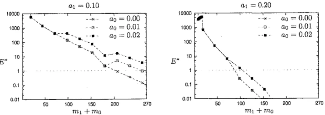
Weshow$E^{*}$$(n, m_{1}, m_{0}, a_{1}, a_{0})$for two combinations ofparameters$n$and$m_{1}/m_{0}$ corresponding
toBCWandHEARTin Figs. 1 and 2, respectively. Each contains two graphs, where the left(resp.,
right)graph is for$a_{1}=$O.JO (resp.,$a_{1}=0.20$). In each graph, the horizontal (resp., vertical) axis represents$m_{1}+m_{0}$ (resp.,$E’$) and the threecurvescorrespondto different values of$a_{0}$
.
Note thatthe vertical axis is the logarithmic scale.
$E^{*}$ appears to be an approximately monotone decreasing function of
$m_{1}+m_{0}$
.
As observedfrom the figures, $E^{*}$issufficientlysmall(i.e., less than 1)
as
$m_{1}+m_{0}$is larger than at most several
hundred, Among the examined values of$m_{1}$ (resp., $m_{0}$), let us denote by $M$
;
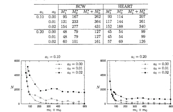
(resp., $M_{0}^{*}$) the smallest value that attains $E^{*}\leq 1$. Table 1 shows $(M_{1}^{*}, M_{0}^{*})$ for each parameter combination$a_{1}=0.10$ $a_{1}=0.20$
10000 10000
$000 $\backslash ^{\backslash }\backslash -\mathrm{g}^{\backslash }\backslash \mathrm{l}\backslash \mathrm{g}\iota_{1}$ $\mathrm{t}^{\mathrm{c}\iota^{\backslash }’-}\backslash \backslash \backslash .\backslash$
$- \mathrm{s}--*--$ $a_{0}a_{0}==0.010.00$ 1 $000\mathrm{t}00$ $\backslash$ $-$) $6-\bullet \mathrm{O}^{\cdot}$ $a_{0}=0.\mathrm{o}\mathrm{o}$ $ao=0.\mathrm{O}1$ as$=0.02$ -a $a\mathrm{o}=0.02$ 100 $\nwarrow 0^{\cdot}\mathrm{r}$ $\mathrm{t}$, $\iota_{\backslash }$
$E’$ $10\uparrow$ $\backslash \mathrm{b}^{\mathrm{b}}\nwarrow\backslash ;_{l}\backslash ^{\mathrm{E}\mathrm{J}}\nwarrow_{\backslash }\mathrm{B}\mathrm{x}_{\backslash }\backslash .\backslash 1$ $E^{*}$ $701$ $\iota_{\aleph_{1}^{\backslash }}\iota_{1}^{-}\backslash \backslash \backslash$
$[searrow]\backslash$
$\grave{\mathfrak{g}}$ $\vee \mathrm{r}$
$\backslash \backslash \mathrm{o}\mathrm{e}_{1}1$
01
$\mathrm{t}_{\backslash }\backslash \backslash$ $\tau_{\mathrm{J}}\{\mathrm{D}$ i3a $\backslash .-\cdot\backslash$ 07 $\backslash$ $\iota_{1}\backslash \mathrm{D}1_{\iota}$ $.- \mathrm{r}_{\backslash }$ 001 0OI 100 200 300 400 683 100 200 300 400 683 $m_{1}+$
mo
$m_{1}$$+m_{0}$Figure 1: $E^{*}(n, m_{1}, m_{0}, a_{1}, a_{0})$ with $n=13$ and $m_{1}/m_{0}=$ 239/444 (corresponding to data set
BCW)
Ql $=010$ $a_{1}=0.20$
10000 10000
1000 $\backslash \backslash \backslash \mathrm{r}\backslash \backslash \backslash _{\bullet\backslash --arrow}$ $—–\succ \mathrm{I}3$
$a_{0}=0.\mathrm{o}\mathrm{o}$ 1000 $p_{\iota_{\mathfrak{l}}}\mathrm{A}_{\backslash }$ $-$ ) $\epsilon---- \mathrm{B}$ $a_{0}=0.\mathrm{o}\mathrm{o}$ $a_{0}=0.01$ $a_{0}=0.01$ $a_{\mathrm{O}}=0.02$ $a_{0}=0.02$ $E^{*}$ $10010$ $\backslash$
$\backslash -\mathrm{x}_{\backslash }^{\backslash }\backslash \backslash \backslash \mathrm{x}_{\backslash }^{-}\backslash \backslash \mathrm{q}_{\backslash \backslash }\backslash \backslash \backslash \cdot.\backslash \backslash \backslash \wedge-\bigwedge_{13}\backslash \backslash$
.
$B^{\mathrm{r}}$$70010$ $\backslash \backslash _{\backslash _{\backslash }}\backslash _{\backslash ,\backslash \backslash }$
,
$\backslash \mathrm{a}_{\mathrm{c}}’$
’
-t3 $\backslash \backslash$
1 $\backslash \sim\kappa_{\sim}$ $\mathrm{u}$ 1
$\backslash 1\backslash \backslash$ $\backslash \backslash \}\iota_{\backslash }\backslash$
$\backslash \rangle \mathrm{t}$
$\backslash \mathrm{h}\backslash \backslash \backslash .\backslash \backslash$
0101 $\backslash$
$\backslash 1_{\backslash }\backslash 1$ $\backslash$
001 001
50 100 150 200 100 150 200 270
$m_{1}+m_{\beta}$ Ml$+m_{0}$
Figure 2$\cdot$
$E^{*}(n, m_{1}, m_{0}, a_{1}, a_{0})$ with $n=10$ and $m_{1}/m_{0}=$ 120/150 (corresponding to data set
HEART)
Let us mention the values of$\max\{M_{1}, \mathrm{J}/I_{1}(t)\}$ and $M_{0}(s)$ of Theorem 6 as upper bounds of
$M_{1}^{*}$ and $\mathrm{J}/I_{0}^{*}$, respectively. For given$n$, $a_{1}$ and $a_{0}$, we compute$M_{1}$, $\Lambda I_{1}(t)$ and$M_{0}(s)$ by setting
$p=q=1/2^{n}$ and $\epsilon$ $=1/n$. We take $t$ and $s$ such that they minimize $\max\{M_{1}, M_{1}(t), M\mathit{0}(s)\}$
amongthose$t=\ell \mathrm{x}10^{-3}\in(0, a_{1}(1-1/e^{2})]$ and$s=\ell’\mathrm{x}$$10^{-3}\in(0, a_{1}-a_{0}-t]$for natural numbers
$f$and$l’$; inthisexperiment,weobtain such $(\mathrm{i}, s)$ by the sim pleenumeration. The obtainedupper boundsarenot very tight;e.g.,if $(n_{\rangle}a_{1}, a_{0})=(13,0.10 0.00)$,then$M_{1}=$449.20, $M_{1}(t)=$6036.04
and $M_{0}(s)=$6029.60,while $M_{1}^{*}=95$ and$M_{0}^{*}=167$ from Table 1 It indicates that Theorem 1
and 2 do notalways givetightbounds.
3.3
Number
of
Good Rules in Real Data
For given real data sets and ($a_{1}$,$a_{0}\rangle$, we would like to observe how the number of good rules changes as$m_{1}$ and $m_{0}$ increase and compare its tendency with the values of$M_{1}^{*}$ and
$M_{0}^{*}$ of the lastsubsection. In order to simulate the situation where we have smaller number of examples than the original data set, we randomly sample $X_{1}\subseteq X_{1}^{*}$ and $X_{0}\subseteq X_{0}^{*}$ with $|X_{1}|=m1$, $|X_{0}|=m0$
and$m_{1}/m_{0}=m_{1}^{*}/m_{0}^{*}$, and generate$(a_{1}, a_{0})$-good rules in $X=X_{1}\cup X_{0}$. Werepeat this process
$\tau$times and take the average $N$ofthe numbers of$(a_{1}, a_{0})$-good rules. In this experiment,we
use
$\tau=100$.Weshow$N$forBCWandHEARTin Figs.3 and4, respectively. Note thatthevertical
axes
inthese figures
are
notthelogarithmic scaleincontrast to Figs. 1 and 2. In each graph of the figure for HEART, the threecurves
overlapTable 1: $(M_{1}^{*}, M_{0}^{*})$for variousparametercombinationscorresponding to real datasets $a1=0.10$ $a_{1}=0.20$ 6000 6000 4000 4000 $N2000$ $N2000$ 0 0 $m_{1}+m_{0}$
Figure3: The number $N$ofgoodrules fordata setBCW
For dataset BCW, we seethat the number $N$ ofgenerated good rules does not change much
when $m_{1}+m_{0}\geq\Lambda’I_{1}^{*}+M_{0}^{1^{\zeta}}$, while it drastically decreases when $m_{1}+m_{0}<M_{1}^{*}+M_{0}^{*}$, for all
combinations of$(a_{1}, a_{0})$. Weobserve that if$m_{1}$ and$m_{0}$ aresmall (e.g., 10to30), thenmorethan
10 superficial good rulesareextracted, while$X^{*}$containsat most2000real good rules.
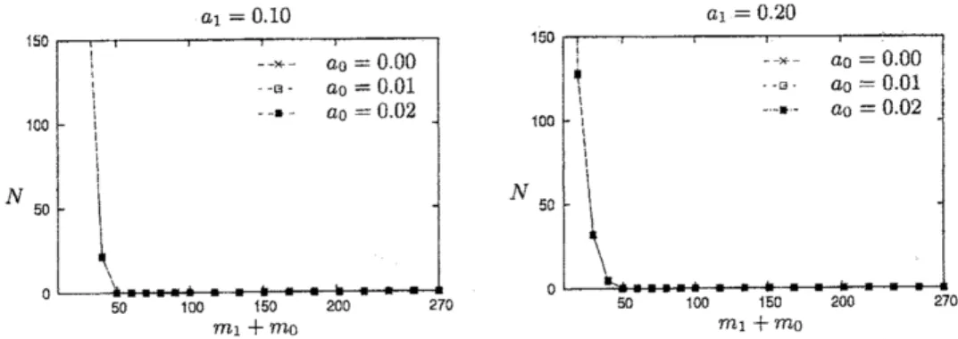
For data set HEART, $N$ becomes 0 with $(m_{1}, m_{0})$ which are smaller than $(M_{\mathit{1}_{1}}’, M_{0}^{*})$. Some
datasetsdo notcontaingoodrulesalthoughtheyhavesomeregularitiesorstructures; forexample, suppose sucha dataset$X=\mathrm{B}^{\tau\iota}$ and each example$x\in X$is labeled
$\omega$ bythepar$ity$function;
$\omega$ $=$ $\{$ 1 if
$\sum_{j=1}^{n}x_{j}$isodd,
0otherwise. (15)
Clearly, $X$ does not have$(a_{1}, a_{0})$-good rules under reasonable $(a_{1}, a_{0})$ although it has the rule of
(15). In the caseof such data sets, it is important to detect that there is no good rule of our
definition. Figs: 5 and 6 show that, for these data sets, it is sufficient for us to have $M_{1}^{*}$ true
examplesand$M_{0}^{*}$ false examples in order to seethatthere isnogoodrule.
The aboveresultsjustifyourclaimonthesize ofthedata set needed to generate reliable good rules. However,$\max\{\mathrm{J}/I_{1}, M_{1}(t)\}$ and$M_{0}(s)$
are
not very good as upper bounds of$M_{1}^{*}$ and$M_{0}^{*}$, respectively. Itisourfuture work to derive tighter upper bounds.4
Conclusion
Inthispaper, weconsider howmanyexamplesareneeded in data sets for extracting reliable good
rules. Our claim is that the data set should containexamples morethan the value such that a
random data set has good rules very rarely. We derive arequired amount of true examplesas
$\max\{M_{1}, M_{1}(t)\}$ and offalse examples as $M_{0}(s)$
.
We then showsome
computational studies to$\mathrm{I}50$ $00 $N$ $a_{1}=0.10$ $a_{1}=0.20$ $\mathrm{I}50$ $\iota_{1}$ ‘ 100 $||\iota_{\mathrm{I}}\downarrow|||$ 50 $\xi|$ 150 $–\kappa-$ –B- $a0=0.01$ $a_{0}=0.01$ $a0=0.00$ 100
$\dagger_{1}|‘|||$ $-\cdot-*\sim--k-- \mathrm{B}-$
$a0=0.00$ $a0=0.02$ $a\mathit{0}=0.02$ $||\iota_{\mathfrak{l}}$ $N50$ $|\{$ $\backslash$ 0 50 100 $50 200 270 0 50 100 150 200 270 $m_{1}+m\mathit{0}$ $m_{1}+m\mathit{0}$
Figure4: The number$N$of good rulesfor data setHEART
Acknowledgments
We areindebted to Prof. Toshihide Ibaraki of KwanseiGakuinUniversity, Japan,and Prof. Endre
Boros of Rutgers University, USA, for a number of helpful comments and suggestions. This work
wassupported byGrant-in-Aidfor Scientific ResearchonPriority Areas “Comparative$\mathrm{G}\mathrm{e}\mathrm{n}\mathrm{o}\mathrm{m}\mathrm{i}\mathrm{c}\mathrm{s}^{)2}$ fromthe MinistryofEducation, Culture, Sports, Scienceand Technology ofJapan.
References
[1] R. Agrawal, T. Imielinski, A. Swami, “Mining Association Rules between Sets of Items in Large Databases”, ACM SIGMOD
Conference
onManagementof
Data, 1993[2] N.Alon, J. H. Spencer,P.Erdos,eds., “The ProbabilisticMethod”, , John Wiley
&
Sons, 1992[3] H. Chernoff, “A Measure of the Asymptotic EfficiencyforTests of a Hypothesis Basedonthe
Sum of
Observations”
, Annalsof
MathematicalStatistics, vol. 23 (1952),pp. 493-509[4] U. Fayyad, G. Piatetsky-Shapiro, S. Padhraic, “Prom Data Mining toKnowledge Discovery
in Databases”, AI Magazine, vol. 17,No. 3 (1996), pp. 37-54
[5] K. Haraguchi, T. Ibaraki, E. Boros, “Classifiers Based on Iterative Compositions of Fea-tures”, Proc, 1st International
Conference
on Knowledge Engineering and Decision Support(TCKEDS2004), Porto,Portugal (Jul, 2004), pp. 143-150
[6] W. Hoeffding, “Probability Inequalities forSumsof Bounded RandomVariables”, Journal
of
American StatisticalAssociation, vol.58 (1963), pp. 13-30
[7] Y. Li,R. P. GopaLan, “Effective Sampling for Mining Association Rules”, LNAI 3339, G. I. Webb and X. Yu eds. (2004), Springer-Verlag, pp.
391-401
[8] H. Toivonen, “SamplingLarge Databases for AssociationRules”, Proc. 22nd VLDB
Confer-ence, Bombay, India (1996), pp. 134-145 [9] C.L. Blake,C. J. Merz, eds.,
“UCIRepositoryof MachineLearningDatabases”,http:$//\mathrm{w}\mathrm{w}\mathrm{w}$.ics.uci.$\mathrm{e}\mathrm{d}\mathrm{u}/\sim \mathrm{m}\mathrm{l}\mathrm{e}\mathrm{a}\mathrm{r}\mathrm{n}/$ Repository.html, 1998
[10] T. Uno, M. Kiyomi, H. Arimura, “LCM ver 2: Efficient Mining Algorithms for $\mathrm{F}\mathrm{r}\mathrm{e}\mathrm{q}\mathrm{u}\mathrm{e}\mathrm{n}\mathrm{t}/$ $\mathrm{C}\mathrm{l}\mathrm{o}\mathrm{s}\mathrm{e}\mathrm{d}/\mathrm{M}\mathrm{a}\mathrm{x}\mathrm{i}\mathrm{m}\mathrm{a}\mathrm{l}$ itemsets”,, Proc, IEEE
ICDM’04
Workshop FIMF04,2004[11] G. Yang) “The Complexity ofMining Maximal Frequent Itemsets and Maximal Frequent
Patterns”, , Proc. 10thACM SIGKDD