A $Matlab$ Problem-Solving Environment for Nonlinear Systems Education in Mathematics, Physics and Engineering (Computer Algebra Systems and Education : A Research about Effective Use of CAS in Mathematics Education)

A Matlab

Problem-Solving

_Environment

_for

Nonlinear

Systems

_Education

_in

Mathematics,

Physics and

Engineering

Akemi

G\’alvez

_Tomida

Department

_of

Applied

Mathematics

and

Comp.

Sciences

University

_of

Cantabria,

Avda.

de

los

Castros

s/n,

E-39005, Santander,

Spain

galveza@unican.es

Abstract

Currently, European countriesareinthe_{process of rethinking their Higher}

Edu-cation systems due toharmonizationeffortsinitiated by Bologna’sdeclaration. This

scenarioof reformsdemandsacompletelynewapproach to the instructionalprocess.

A major issue in this context is the development of better, updated educational

tools and materials specially adapted to the topics under study. This work reflects

author’sexperiencein developingaproblem-solving environment designed forafirst

course on nonlinear systems for undergraduate students of Mathematics, Physics

andEngineering. In this paperthe architectureofthis computer system along with

a description of its main functionalities are briefly reported.

1

_Introduction

Bologna’s

declaration

-

seen

today as the well-known synonym for the whole process

of

reformation

in the

area

of higher education-was signed in 1999 by 29 European

countries with the objective to create “a European space

_for

higher education in order

to enhance the employability and mobility

_of

citizens and to increase the intemational

competitiveness

_of

_{European higher education” [1]. Its upmost goal is the commitment}

freely taken by each signatory country to reform its own higher education system in

order to create overall

convergence

at European level. This process encompasses the

adoption of

a

common

framework

of readable and comparable degrees

as

well

as

the

introduction of undergraduate and postgraduate levels in all countries along with

ECTS

(European _{Credit Transfer System) credit systems to}

_ensure

_a

_{smooth transition from}

one

country’s system to another one, thus enforcing free mobility of students, teachers

and

administrators among

the European countries.

Unquestionably, Bologna’s declaration opened the door to

a

completely

new

scenario

for higher education in Europe. Nowadays, the European countries

are

in the midst of

the process ofrestructuring theirhigher education system in order to fulfill the objectives

such

as

the definition of the

new

curricula and grading systeins. However, the upcoming

changes go far beyond these structural changes, as the personal development of students and teachers is also at the root of this

new

concept ofeducation. For instance, students

in this

new

model

are no

longer passive actors of the learning process.

On

the contrary,

Bologna’s declaration emphasizes the concept ofself-learning

so

that students

are

getting

more and more involved in their

own

learning.

An important issue in this process is to provide students with

a

good collection of scholar materials that enable them to accomplish the learning process by themselves.

During the last few years, the author has been involved in the development ofcomputer

softwarefor

a

first

course on

nonlinear systems for undergraduate students of

Mathemat-ics, Physics and Engineering. As

a

result,

a

new

Matlab problem-solving environment

designed to attain the demands of this

new

situation has been created from scratch. In

this paper the architecture of this computer system along with

a

description of its main

functionalities

are

briefly reported.

2

Nonlinear

(Chaotic)

Systems

The analysis of chaotic dynamical systems is

one

of the most challenging tasks in

Com-putational Science. Because the chaotic systems

are

essentially nonlinear, their behavior

is much

more

complicated than that of linear systems. In fact, even the simplest chaotic

systems exhibit

a

bulk of different behaviors that

can

only be $f\iota illy$ analyzed with the

help of powerful hardware and software

resources.

The range of different phenomena associated with the nonlinear systems is extremely

varied. Chaos

can

be found in almost any field, ranging from chemical reactions to

elec-tronic circuits and lasers [2, 11], meteorology [16], ecology [18], etc. Nonlinearity appears

in both discrete and continuous systems, which are described by iterated functions and

differential

equations, respectively [15, 19]. That

means

that the accurate analysis of

such chaotic systems requires specialized mathematical tools and techniques, designed

to account for the kind of system involved. This challenging issue has motivated

an

in-tensive development of

programs

and packages aimed at analyzing the

range

ofdifferent

phenomena associated with the chaotic systems.

Among these programs and packages, thosebased

on

computer algebra systems (CAS)

are receiving increasing attention during the last few years. Recent examples can be

found, for instance, in [3, 4, 5, 6, 8] for Matlab, in [7, 9, 10, 12, 13, 14, 21] for Mathematica and in [22] for Maple, to mention just a few examples. In addition to their outstanding

symbolic features, the CAS also include optimized numerical routines, nice graphical

capabilities and- in a few

cases

such

as

in Matlab- the possibility to generate appealing

GUIs (Graphical User Interfaces).

In this paper,

we

describe a problem-solving environment for the analysis of chaotic

dynamical systems. The program,

an

improvement of the system reported in [5, 6] and

implemented in the popular

CAS

Matlab, is suitable for both discrete and continuous

chaotic systems. To this purpose, specialized symbolic and numerical libraries have been developed. Further, to provide end-users with

a

nice navigation and intuitive

access

to

the main methods and routines,

a

powerful graphical

user

interface (also described in

this paper) has been implemented. To show the good performance of this proposal,

some

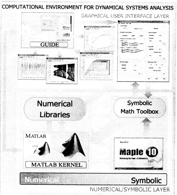
Figure 1: Architecture ofthe system.

3

Program

Architecture

and Implementation

3.1

Program

Architecture

Figure 1 shows the architecture of the program described in this paper. It consists of two

1.

a

$nume^{J}r^{v}ical$-symbolic layer it is basically

a

collection of numerical and symbolic

libraries containing the commands, functions and routines implemented to perform

numerical and symbolic tasks.

2. agraphicaluser

_interface

$(GUI)$ layer. this componentis responsibleforinput/output

windowing, display of graphical output and smooth interaction with the

user.

3.1.1 Numerical-symbolic layer

The nuinerical-symbolic layer is comprised of three different modules, according to the

distinct processes (numerical, symbolic and graphical) to be carried out:

1.

a

set

_of

numericd librames containing the implementation of the commands, func-tions and routines for the

numerical

tasks.

They have been implemented in the

native Matlab programming language. To this aim

we

take advantage of the large

collection ofnumerical routines available in the Matlab kernel such libraries

are

con-nected with. These standard Matlabroutines provide extensive control

on

different options and

are

fully optimized to offer the highest level of performance.

2.

a

set

_of

symbolic routines and

_functions.

They have been implemented by using the

Symbolic Math Toolbox that provides

access

to several Maple routines for symbolic

tasks. This symbolic module is

more

important than it might

seem

at first sight;

for instance, system equations

are

inputted symbolically so that

some

functional operators (such

as

derivatives)

can

be effectively applied. Further, some additional

operators (string manipulation, forward/backward symbolic object-string

conver-sion, symbol replacement and assigmnent, etc.) have

also

been used for symbolic

purposes. It is worthwhile to mention that the Symbolic Math Toolboxis less

pow-erful than the Maple kemel system it comes from. Fortunately, it is also possible

to connect the kemels of Matlab and Maple for very specialized symbolic tasks.

3.

some

graphical commands. The powerful Matlabgraphical capabilities exceed those

comunonly available in other

CAS

such

as

Mathematica and Maple. Although

our

current needs do not require applying them at full extent, they avoid the

users

the

tedious and time-consuming task to implement many routines for graphical output

by themselves. Some nice viewing features such as $3D$ rotation, zooming in and

out, labeling, scaling, coloring and others are also automatically inheritedfrom the

Matlab graphical and windowing systems.

3.1.2 Graphical

user

interface layer

Although the librariesin previous layer

are

oftenenough to meet

our

computational needs,

end-users might be challenged for using them properly unless they

are

really proficient

on

both Matlab syntax and functionalities and

our

implemented routines. This

limita-tion

can

be

overcome

by creating a GUI;

a

well-designed GUI

uses

readily recognizable

visual

cues

to help the

user

navigate efficiently through information. Matlab provides a

powerful mechanism to generate GUIs by using the so-called guide $(GUI$ Development

Ehvironment). This feature is not commonly available in many other CAS

so

far.

it allows end-users to deal with

our

libraries with a minimal knowledge and input, thus

facilitating

its

efficient

use

and

dissemination.

Based

on

this discussion,

a GUI

layer has been implemented.

Some

examples of

typical windows of

our GUI

are depicted in upper part of Figure 1. Some windows

are

for user interaction-typicalIy input acquisition, parameter tuning and option selection

tasks. Others are windows to display graphical output. All them allow an effective

use

of powerful interface tools designed according to the type of entities being displayed

(e.g., drop-down

menu

for a choice list, _{check buttons for Boolean options, text boxes}

for displayingmessages, dialog boxes for input/output

user

interaction, etc.).

Additional

functionalities are

providedinhidden

menus

or

inseparate _{windows which}

can

beinvoked

at will ifneeded

so as

to keep the main windowstreamlinedand uncluttered. Forinstance,

all graphical output is displayed in separate windows

so

that the

information

is better

organized and flows in

a

natural and intuitive way. As

a

result, the system presents

a

GUI that

is

both

aesthetic and very

functional

to the

user.

3.2

Implementation

_issues

Regarding the_{implementation, thuis program has been developed by the author in Matlab}

$v2007b[17]$ _running

_{on Windows}

_{XP operating system by using}

_{a PC}

_{with Intel}

_Core

2 Duo processor at 2.4

GHz.

and

2 GB

of

RAM.

However, the program supports many

different

platforms, such

as

PCs (with Windows $9x$, 2000, NT, Me, XP and Vista) and

UNIX workstations. A version for Apple Macintosh with Mac OS X system is also

available provided that

Mac

Xll (the implementation of the X Window System that

makes it possible to

run

Xll-based applications in Mac

OS

X) is properly installed and

configured. Figures in this paper correspond to the

PC

platform version.

The graphical tasks are performed by using the Matlab GUI for the higher-level

func-$tion\llcorner s$ (windowing, menus,

or

input) while the built-in graphics Matlab commands

are

applied for rendering purposes. The numerical kernel has been implemented in the

na-tive _{Matlab programming language, and the symbolic kernel has been created by using}

the commands ofthe Symbolic Math Toolbox.

4

Discrete

Systems

The program

described

in previous _{section is well suited for dealing with both discrete}

and continuous dynammical systems. This section illustrates the

use

of this software for

the

case

of

discrete

systems.

4.1

Fixed points and stability

Given

an

iterated map defined by

a

function $f(x)$, a

fixed

_point $x^{*}$ of$f(x)$ is a point that

ismapped to itself by thefunction, $i.e$. $f(x^{*})=x^{*}$_. Let’s considerfor example thelogistic

map given by $x_{n+1}=\lambda x_{n}(1-x_{n})$, where $n\in$ IN and $\lambda$ is

a

system parameter, usually

taking values

on

the interval [0,4]. The logistic map became popular following

a

seminal

paper by the biologist Robert May in 1976 [18], where he introduced the discrete version

of

a

demographic model due to Verhulst. Roughly, $x_{n}\in[0,1]$ represents the population

a $arrow$

ffi $\zeta xmbs$ $Io*$ $M$

Systr Equim

$x(n\cdot 1)$.

$|mt,dQ^{\cdot}Y(n).t\uparrow Y(\cap))$ $Pu 6tcr$

Dynmcd$Sy\#-$Andvsis $\llcorner Y\sim unov\in xp\alpha*$ $\Re..bllityotFlx\cdot dPo1mF|xedP\alpha|s.$

. $\theta*\iota_{V}$

.

$|\overline{\underline{Co\mathfrak{m}pu!\epsilon}}|\wedge$ $p_{Qn’\alpha r}lrdPr$

$x(0)\Rightarrow$

lxdPc$l1$) $\approx 0$ $\vee \mathfrak{n}$

.

$\vee lh$

.

$b\cdot(l\cdot\cdot bd\cdot)$ $\sim 1$ $–\triangleright$ St $b1$

.

$lmbd$

.

$-l$ $or$ $1\cdot*bd\cdot\cdot l$ $–\triangleright S\cdot ddl$

.

$\infty\alpha\backslash$

$b\cdot\prime l\cdot\cdot bd\cdot)$ $\triangleright\downarrow--\succ Un*t\cdot b1$

.

$l\cdot\wedge bd\cdot\cdot$$0$ $-\succ$ $S\backslash lp\cdot r*CUlo$

..$c\alpha_{W}\alpha m$ $-$ $PxdPt(Z)$ $\cdot t1\cdot*bd\cdot-1)/1\cdot\cdot bd$

.

$WP\alpha t$ $x(0)$

.

$b*(\tilde{-}*1\cdot\cdot bd*\}$ 4 1 $–>$ St$*b1$

.

$1\cdot lbd$

.

.

1 or lmbda

.

3 $–$, Saddle I

$b\cdot t-Z+1\cdot*bd\cdot)$ $\succ 1--\geq un\mathfrak{s}C$ab$l\circ$

$1\cdot-bd$

.

.

$Z–\backslash$ Supa$r$ _$*1$

.

$p\sim’\alpha ervdr$

.

$a\dagger^{-}uc\circ 0\alpha\vee-$ $rwPo t$ $x(0)$

.

$p_{rdn\alpha*r}$ $vn$

.

$\vee fh$

.

$|\overline{\alpha \text{く}}|$ $xh$

.

$x\prime \mathfrak{n}=$ $|\overline{(\supset\ltimes}|$ $\#rSp\kappa oCrW$ $\square 1D$ _{ロ 20} $\square 3D$ $i\urcorner 1-Po t$ $x(0)$

.

$P\alpha’\alpha uw\iota r$

.

$\overline{\infty\alpha \text{く}}|$ $\overline{\infty c\infty}|||\overline{ckoe}||\overline{\}sr}|$

Figure 2: Fixed points and stability of the logistic map.

system evolves among

a

number of different situations, from the population eventually

dying to stabilizing

or

changing chaoticaly (see [18] for

more

details).

The program described in

this

paper

can

compute the fixed points of any iterated map. To do so,

_we

must enter the system equation

as

shown in Figure 2. Note that

the equation is given in a mathematical-looking way so that it can be subsequently processed for further symbolic-numerical calculations. For instance, we can also analyze

the stability of fixed points, by computing the eigenvalue of the fixed point, given by:

$\phi=[\frac{df(x)}{dx}]_{x=x^{*}}$ The fixed point is stable if $|\phi|<1$, neutral if $|\phi|=1$, unstable if

$|\phi|>1$, and superstable if $|\phi|=0$. The fixed points for the logistic map

are:

$x=0$ and

$\lambda-1$

$x=\overline{\lambda}$. Figure 2 shows the fixed points ofthe logistic map along with their stability

analysis in terms of the $\lambda$ parameter.

4.2

Bifurcation diagrams

Depending on the $\lambda$ value, the logistic map evolves among a number of different

Figure 3:

Bifurcation

diagramof the logistic map

on:

(left) interval $[0,4]$; (right) interval

[3.82, 3.86].

Figure 4:

Bifurcation

diagram of the cubic map

on

the interval [1, 4] for the initial conditions: (left) $x_{0}=0.5$; (right) $x_{0}=-0.5$.

the possible long-term values (fixed points

or

periodic orbits) of

a

system

as a

function

of a

system parameter. Figure 3 (left) shows the

bifurcation

diagram of the logistic map

for $\lambda\in[0,4]$

.

The initial input consists of the initial point _{$x_{0}$} and the initial and final

values of the system parameter. The bifurcation diagram is

a

fractal: if you

zoom

in

on

the value $\lambda=3.825$ and focus

on one

branch of the _{diagram, the situation nearby looks}

like

a

shrunk and slightly distorted version of the whole diagram,

as

shown in Figure 3 (right). This is

an

example of the deep and ubiquitous connection between chaos and

fractals.

Figure 5: (left) Lyapunov exponent of the logistic map on the interval $[0,4]$; (right) close

up

on

the interval [3.2, 4].

depend on the initial values of the system variable, $x_{0}$. This happens, for instance, for

the cubic map, given by: $x_{n+1}=(1-\mu)x_{n}+\mu x_{n}^{3}$. This system has two fixed points of

the form $x_{1,2}=\pm\sqrt{\frac{\mu-1}{3\mu}}$, meaning that there is

no

single value to display the whole

bifurcation diagram. Figure 4 displays the two bifurcation diagrams associated with

this map, obtained from two different initial conditions for the system variable, namely

$x_{0}=0.5$ (left) and $x_{0}=-0.5$ (right). As the reader

can

see, there

are

two missing

branches of the period-4 orbits in each diagram, so both pictures

are

complementary

each other.

4.3

Lyapunov exponents

One indication of chaoticity is the so-called sensitivity to initial conditions, meaning

that two initially closed arbitrary trajectories diverge exponentially over the time. The

Lyapunov exponent (LE) of a dynamical system is the number that characterizes the

rate of separation of these infinitesimaJly close trajectories along a given direction. Of

course, the rate ofseparation

can

be different fordifferent orientations of initial separation

vector, leading to

as

many Lyapunov exponents

as

thenumber of dimensions of the phase

space. LEs

are

intensively applied to analyze the behavior of nonlinear systems, since

they indicate ifsmall displacementsoftrajectories

are

alongstable or unstable directions.

In short,

a

negative LE is

an

indicator of regular (stable) behavior while a positive LE

means

that the orbit is unstable and chaotic.

Our program allows

us

to compute the Lyapunov exponents in a very easy way; the

initial input is given by the initial point for the system variable and the interval for the

system parameter. Figure 5 (left) depictes the Lyapunov exponent of the logistic map

for the system parameter on the interval $[0,4]$. Comparison of this picture with Figure 3

(left) shows that negative values for the LE

are

an

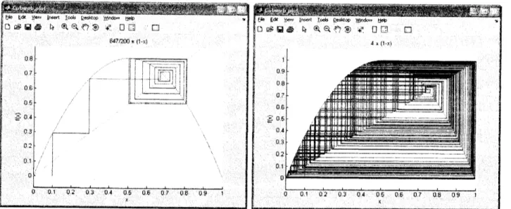
indication of regular behavior, while

Figure 6: Cobweb plot of the logistic map: (left) $\lambda=3.235;$ (right)$\lambda=4$

.

for $\lambda=2$, meaning the existence of a _{superstable fixed point. Figure 5 (right) shows}

a

magnification _{of the figure}

_on

_{the left for the interval [3.2, 4]. We}

_{can see}

_{that the}

LE is positive for $\lambda>3.569\ldots$ except by the existence of

some

_{periodic windows, thus}

explaining very well the bifurcation diagram in Figure 3 (left).

4.4

Cobweb

plot

A

cobweb plot is

a

graphical procedure especially suited to analyze the qualitative be-haviourof

one-dimensional

iterated fumctions. Cobwebplots

are

usefulbecause theyallow

to determine the long-term evolution of

an

initial condition under repeated application

of

a

map. Figure 6 shows two cobweb plots_{for the logistic map and the initial conditions}

$\lambda=3.235$ (left), and $\lambda=4$ (right). The first

one

shows the

case

_of a _{period-2 orbit}

(represented by

a

rectangle) while the second

case

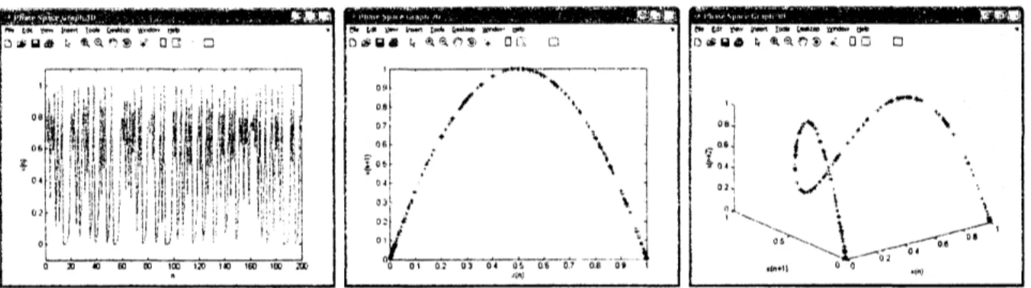
is a chaotic orbit.

4.5

Phase

space

graph

A

very

powerful strategy to analyze chaotic systems is to

use

the so-called phase space

graph By this

we

mean

a collection of pictures associated with the orbit of

a

given point

$x_{0}$ and embedded into

different n-dimensional

spaces. For $n=1$ we get the signal ofthe

orbit, i.e. the sequence of iterates $\{x_{n}\}_{n}$

over

the time. Such sequence is usually called

the time

serees.

For $n=2$ _{the graph} is obtained by representing the sequence ofiterates

$\{x_{n+1}\}$ vs. $\{x_{n}\}$, for $n=3$,

we

represent the sequence of iterates _{$\{x_{n+2}\}$} vs.

$\{x_{n+1}\}$ and

$\{x_{n}\}$ and

so

on.

Figure

7 uses

the phase space graph to analyze the chaotic behavior of the logistic

mapfor$\lambda=4$

.

Thesepictures illustrateperfectly how the_{chaotic behavior looks}

like. On

theleft, the signal of the orbit is displayed. As discussed above, a characteristic of chaos

is that chaotic systems exhibit a great sensitivity to initial conditions. A

common source

of such sensitivity to initial conditions is that the map represents

a

repeated folding and

Figure 7: (left to right) lD, $2D$ and $3D$ phase space graph for the logistic map.

logistic map, represented in Fig. 7 (middle), gives

a

two-dimensional phase diagram of

the logistic map showing the quadratic

curve

ofits iterated equation. We

can

also embed

the

same

sequence in

a

$3D$ phase

space,

in order to investigate

a

deeper structure of the

map. Figure 7 (right) shows how initially nearby points begin to diverge, particularly in

those regions corresponding to the steeper sections of the plot.

5

Continuous Systems

In this section

we

show

some

applications of the program through illustrative examples

forthe

case

ofcontinuous systems. In thuis work

we

restrict ourselves to the

case

of

finite-dimensionalflows, whuich

are

mathematically describedby systems of ordinary differential

equations.

5.1

Symbolic-numerical

analysis

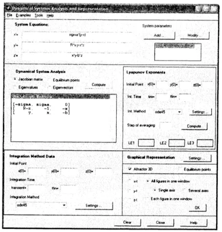
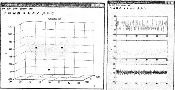
Figures

8-11

show screenshots of

a

typical session for analyzing $3D$ continuous systems.

The session workflowis

as

follows: firstly, the

user

inputs the system equations expressed

symbolically. For instance, in Figure 8

we

consider thefamous Lorenz system [16], given

by: $(x’, y’, z’)=(\sigma(y-x), (R-z)x-y, xy- bz)$ where $\sigma,$ $R$ and $b$ are the system

parameters. The program includes a module for the computation ofthe Jacobianmatrix and the equilibrium points of any finite-dimensional flow. The Jacobian matrix is

a

square matrix whose entries

are

the partial derivatives of the system equations with

respect to the system variables. If no value for the system parameters is provided, the

computation is performed symbolically and the corresponding output depends

on

those

system parameters. The equilibrium points and the eigenvalues and eigenvectors of the

system

can

also be computed in

a

similar way.

Figure 8 shows the symbolic Jacobian matrix for the Lorenz system, which depends

not only

on

thesystem parameters butalso

on

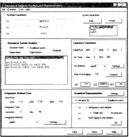
thesystemvariables. Once

some

parameter

values

are

given ($\sigma=10,$ $R=60$ and $b=8/3$ in this example), the Lyapunov exponents

(LE) ofthesystem

can

be numerically computed. To thispurpose, anumerical integration

method is applied [20]. The corresponding options and parameter values are shown in

Figure 9. The numerical values of these LE

are

1.4,0.0012 and-15 respectively. Their

Figure 8: Symbolic Jacobian matrix for the Lorenz system.

Roughly speaking, LEs

are

a generalization of the eigenvalues for nonlinear flows. In

particular, a negative _{LE indicates that the} trajectory evolves along the stable direction

forthis variable (and hence, regularbehaviorfor that variable isobtained) whileapositive value indicates

a

chaotic behavior.

5.2

Visualization

of

chaotic attractors

Since

in our example

_{we find}

positive LE, the system exhibits a chaotic behavior. This

factisevidencedin Figure 11 (left) where the corresponding attractor and the equilibrium

pointsof the Lorenz system for

our

choice of thesystem parameters

are

displayed. Their corresponding numerical values

are

shownin the mainwindow

of

Figure9. Finally, Figure

11 (right) shows the evolution ofthe system variables

over

the time from $t=0$to $t=50$

.

In order to display the attractor and/or the evolution ofthe system variables

over

the

time (like in Figure 11),

some

kind of numerical integration is required. The program in this paper allows end-users tochoosedifferent numerical integration methods [20],

includ-ing the

classical

Euler and 2nd- and $4th$-order Runge-Kutta methods (implemented by

the author) along with

some more

sophisticated methods from the Matlab kemel such

as

ode45, ode23, ode113, ode$15s$, _ode$23s$, _ode$23t$ and _ode$23tb$ (see [17] for details).

Some

input required _{for the numerical integration (such}

_as

_{the initial point and the integration}

time) is also given at this stage. By pressingthe “NumericalIntegrationsettings” button,

Ek $E\cross wvusI’*$ $M$

Systm$E\eta udW$

.

-. $x$

.

$\Psi^{\mathfrak{n}obx|}$ $\mu$ $R.\nu*x.$. :. $xyb^{\backslash }$ $-\sim-7_{\}$ System wrdr$s$ $1rA9dlrTm$ $ur$

.

$0$ $M\sim$ 50 $|n_{C}9dr$Nethod ode45 $su|r9$ $|$

$h\star$

.

An$u\cdot\cdot\n$onewndos

$y^{1}$

.

$Sr*$am $Se$veielaxes

$p|$ $\mathbb{E}aeh1\cdot e\mathfrak{n}$one$1W1\omega$

OK $|$

Cm $|$ _$cb,$

.

$|$ _$H*$ $|$

Figure 9: Equilibrium points and Lyapunov exponents for the Lorenz system.

Figure 10: Temporal evolution of the Lyapunov exponents for the Lorenz system.

maximum stepsize and refinement, the computation speed and others)

can

be set up in

a

separate window. Then the

user

proceeds with the graphical representation stage, where

he$/she$

can

display the attractor ofthe dynamical system and/or the evolution of any of

the system variables

over

the time. Such variables

can

be depicted

on

the

same

or on

different

axes

and windows. The“Graphical Representation settings” button opens

a

new

window where different graphicaloptions such

as

the line width and style, markers for the

Figure $\ovalbox{\tt\small REJECT}\ovalbox{\tt\small REJECT}\cdot r_{O^{r}C17}lrs)^{r}SCem$

.

$(|_{t^{J}}fC)c\dagger\iota$aot_{$1C_{Cv}^{\neg}fCractol$}. and equilibrium points; (right)

tempo-ral $evolutt_{O^{n}}o^{f}s\gamma sCc\tau r\iota var\iota$ablcs.

Figure 12: Chaotic attractors of $3D$ flows: (top-left) Lorenz system; (top-right) _R\"ossler

output shown in Figure 11 where the chaotic attractor and the temporal evolution of the

system variables

are

displayed.

Figure 12 shows the chaotic attractors of four distinct nonlinear flows: Lorenz system

for

weather forecasting, R\"ossler chemical reaction, Van-der-Pol Duffing oscillator and Chua’s electronic circuit (see [19]

for further

information

about

these systems).

Acknowledgments

The author would like to express her sincere acknowledgment and appreciation to Prof.

Setsuo Takato for his kind invitation to participate in this RIMS workshop and visit the

lovely city of Kyoto, and for creating such

a

friendly atmosphere during all my stay in

Japan. I really hope we

can

meet again very soon.

This research has been supported by the Computer

Science

National Program of

the Spanish Ministry of Education and Science, Project Ref.

#TIN2006-13615

and the

University of Cantabria.

References

[1] The Bologna Declaration

on

the Europeanspace forhigher education:

an

explanation.

Association ofEuropean

Universities&EU

Rectors’ Conference (1999) pp. 4 (available

at: $http.\cdot//ec.europa.eu/education/policies/educ/bologna/bologna.pdf)$.

[2] Chua, L.O., Komuro, M., Matsumoto, T.: The double-scroll family. IEEE $\mathcal{I}hnsac-$

tions

on

Circuits and Systems, 33, (1986)

1073-1118.

[3] Dhooge, A., Govaerts, W., Kuznetsov, Y.A.: Matcont: A Matlab package for

nu-merical

bifurcation

analysis of

ODEs.

ACM

Transactions on

Mathematical Software,

29(2) (2003)

141-164

[4] Dhooge, A., Govaerts, W., Kuznetsov, Y.A.: Numerical continuation of fold

bifurca-tions of limit cycles in MATCONT. Lecture Notes in Computer Science, 2657 (2003)

701-710

[5]

G\’alvez, A.:

Numerical-symbolic Matlab programfor the analysisof three-dimensional

chaotic systems. Lectures Notes in Computer Science, 4488 (2007) 211-218

[6] G\’aJvez, A.: Matlab toolbox and GUI for analyzing one-dimensional chaotic maps.

Intemational

_Conference

on Computational Science and Applications, ICCSA2008,

IEEE Computer Society Press, Los Alamitos, CA, (2008)

211-218.

[7] G\’aJvez, A., Iglesias, A.: Symbolic/numeric analysis of chaotic synchronization with

a

CAS.

Future Genemtion Computer Systems 25(5) (2007) 727-733

[8] Govaerts, W., Sautois, B.: Phase response curves, _{delays and synchronization in}

Matlab. Lectures Notes in Computer Science, 3992 (2006) 391-398

[9] Guti\’errez, J.M., Iglesias, A., Gu\’emez, J., Mat\’ias, M.A.: Suppression ofchaos through

changes in the system variables through Poincar\’e and Lorenz return maps.

[10]

Guti\’errez,

J.M., Iglesias, A.: A

Mathematica

package for theanalysis and control of chaos in nonlinear systems. Computers in Physics, 12(6) (1998) 608-619

[11] Iglesias, A.: A

new

scheme based on semiconductor lasers with phase-conjugate

feedback for cryptographic communications. Lectures Notes in Computer Science,

2510

(2002)

135-144

[12] Iglesias, A.,

G\’alvez,

A.: Analyzing the synchronizationofchaotic dynamical systems

with

Mathematica: Part

I.

Lectures

Notes in ComputerScience, 3482 (2005)

472-481

[13] Iglesias, A., Ga’lvez, A.: Analyzingthe synchronizationofchaoticdynamical systems

withMathematica: Part II. Lectures Notes in Computer Science, 3482 (2005)

_482-491

[14] Iglesias, A.,

_G\’alvez,

_{A.: Revisiting}

_some

_{control schemes for}

_chaotic

_{synchronization}

with Mathematica. Lectures Notes in Computer Science, 3516 (2005) 651-658

[15] Lauwerier, H.A.:

One-dimensional

iterative maps. In: Chaos. Holden, A.V. (ed.).

Manchester

University Press,

Manchester

(1986)

[16] Lorenz, E.N.,

Deterministic

nonperiodic flow, Joumal

_of

Atmospheric Sciences, 20

(1963)

130-141.

[17] The Mathworks Inc: Using Matlab. Natick, MA (1999)

[18] May, R.M.: Simple mathematical models with

very

complicated dynamics. Nature

261 (1976)

_459-467

[19] Ott, E.: Chaos in Dynamical Systems. Cambridge University Press, Cambridge

(1993)

[20] Press, W.H., Teukolsky, S.A., Vetterling, W.T., Flannery, B.P.: Numerical Recipes

(2nd edition),

Cambridge

University Press, Cambridge, 1992.

[21] Sarafian, _{H.: A closed form solution of the run-time of}

_a

_{sliding bead along}

_a

_freely

hanging slinky.

Lecture

Notes in Computer Science, 3039 (2004)

319-326

[22] Zhou, W., Jeffrey, D.J. Reid,

G.J.:

An algebraic method for analyzing open-loop