Yusuke Watanabe
DOCTOR OF PHILOSOPHY
Department of Statistical Science School of Multidisciplinary Science The Graduate University for Advanced Studies
March, 2010
We often encounter probability distributions given as unnormalized products of non-negative functions. The factorization structures of the probability distributions are represented by hypergraphs called factor graphs. Such distributions appear in various fields, including statistics, artificial intelligence, statistical physics, error correcting codes, etc.
Given such a distribution, computations of marginal distributions and the normalization constant are often required. However, they are computationally intractable because of their computational costs. One, empirically successful and tractable, approximation method is the Loopy Belief Propagation (LBP) algorithm.
The focus of this thesis is an analysis of the LBP algorithm. If the factor graph is a tree, i.e. having no cycle, the algorithm gives the exact quantities, not approximations. If the factor graph has cycles, however, the LBP algorithm does not give exact results and possibly exhibits oscillatory and non convergent behaviors. The thematic question of this thesis is “How do the behaviors of the LBP algorithm are affected by the discrete geometry of the factor graph?” Here, the word “discrete geometry” means the geometry of the factor graph as a space.
The primary contribution of this thesis is the discovery of a formula called the Bethe- zeta formula, which establishes the relation between the LBP, the Bethe free energy and the graph zeta function. This formula provides new techniques for analysis of the LBP algorithm, connecting properties of the graph and of the LBP and the Bethe free energy. We demonstrate applications of the techniques to several problems including (non) convexity of the Bethe free energy, the uniqueness and stability of the LBP fixed point.
We also discuss the loop series initiated by Chertkov and Chernyak (2006). The loop series is a subgraph expansion of the normalization constant, or partition function, and reflects the graph geometry. We investigate theoretical natures of the series. Moreover, we show a partial connection between the loop series and the graph zeta function.
2
I would like to express my sincere thanks to my adviser, Prof. Kenji Fukumizu, for his generous time and commitment. He placed his trust in me and allowed me the freedom to find my own way. At the same time, he made time for discussion on my research every week and gave me excellent feedbacks. I also thank to his helps to improve my writings.
It is a pleasure for me to thank all people in the Institute of Statistical Mathematics who helped my research during my Ph.D. course. Especially, I would like to thank Prof. Shiro Ikeda for his careful reading of the manuscript and helpful comments.
I would like to thank Prof. Michael Chertkov and Dr. Jason Johnson for their hospitality during my stay in Los Alamos National Laboratory and for things they taught me about the belief propagation algorithm.
Last but not least, I would like to thank my parents, Kenjiro and Kanako, for their unwavering support.
This research was financially supported by Grant-in-Aid for JSPS Fellows 20-993 and Grant-in-Aid for Scientific Research (C) 19500249.
3
General Notation
M(r1,r2) set of r1× r2 matrices
hx, yi inner product of vectors x and y: P xiyi
k · k norm
Spec(X) set of eigenvalues of matrix X
ρ(X) spectral radius of X
diag(x) diagonal matrix with diagonal elements xi
∇2 Hessian operator
intΘ interior of a set Θ
sgn(x) sign of a real value x
Ep[φ] expectation of φ(x) under p
Covp[φ, φ′] covariance of φ(x) and φ′(x) under p(x) Corp[φ, φ′] correlation of φ(x) and φ′(x) under p(x) Varp[φ] variance φ(x) and under p(x)
4
Graphs
G undirected graph G = (V, E)
V vertex set
E edge set
H hypergraph H = (V, F )
F hyperedge set
Ni neighborhood of vertex i.
Nα neighborhood of hyperedge α.
di degree of vertex i.
dα degree of hyperedge α.
core(H) core of hypergraph H
e directed edge (undirected edge in chapter 7)
Graphical models
Ψ ={Ψα} set of compatibility functions, graphical model
xi random variable on i∈ V
Xi value set of xi
X Qi∈V Xi
Z partition function, normalization constant
Exponential families
E exponential family
φ(x) sufficient statistics
ψ log partition function
ϕ negative entropy
Λ Legendre map
Θ set of natural parameters
Y set of expectation parameters
Inference family, LBP
I = {Eα,Ei}α∈F,i∈V inference family
φα(xα) = (φhαi(xα), φi1(xi1), . . . , φidα(xidα)) sufficient statistics ofEα θα= (θhαi, θα:i1, . . . , θα:idα) natural parameters ofEα ηα = (ηhαi, ηα:i1, . . . , ηα:idα) expectation parameters ofEα
Θα set of natural parameters ofEα. θα ∈ Θα
Yα set of expectation parameters ofEα. ηα∈ Yα
E(I) global exponential family
F type 1 Bethe free energy function
F type 2 Bethe free energy function
L(I) domain of type 1 BFE function
A(I, Ψ) domain of type 2 BFE function
mα→i message from α to i
µα→i natural parameter of mα→i
Graph zeta
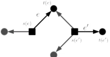
E~ set of directed edges
s(e) starting factor of directed edge e t(e) terminus vertex of directed edge e e ⇀ e′ t(e)∈ s(e′) and t(e)6= t(e′)
PH set of prime cycles of hypergraph H
p prime cycle
re positive integer (dimension) associated with e ri positive integer (dimension) associated with i∈ V X( ~E) set of Cre valued functions on ~E
X(V ) set of Cri valued functions on V
M(u) linear operator on X( ~E), defined in Eq. (3.4) ι(u) linear operator on X( ~E), defined in Eq. (3.9)
Uα diagonal block of I + ι(u)
wαi→j (j, i) element of Wα = Uα−1
D, W linear operators on X(V ), defined in Eq. (3.12)
ζH zeta function of a hypergraph H
ZG zeta function of a graph G
Abstract 2
Acknowledgments 3
1 Introduction 12
1.1 Graphical models . . . 12
1.1.1 Introduction of graphical models . . . 12
1.1.2 Important computational tasks . . . 14
1.1.3 Examples and applications of graphical models . . . 15
1.1.4 Approximation methods . . . 16
1.2 Loopy belief propagation . . . 18
1.2.1 Introduction to (loopy) belief propagation . . . 18
1.2.2 Variational formulation of LBP . . . 20
1.2.3 Applications of LBP algorithm . . . 21
1.2.4 Past researches and our approaches . . . 22
1.3 Discrete geometric analysis . . . 24
1.3.1 Geometry and Equations . . . 24
1.3.2 What is the geometry of graphs? . . . 26
1.4 Overview of this thesis . . . 28
2 Preliminaries 31 2.1 Probability distributions with graph structure . . . 31
2.1.1 Basic definitions of graphs and hypergraphs . . . 32
2.1.2 Factor graph representation . . . 34
2.2 Loopy Belief Propagation algorithm . . . 36 7
2.2.1 Introduction to exponential families . . . 36
2.2.2 Inference family for LBP . . . 40
2.2.3 Basics of the LBP algorithm . . . 42
2.2.4 BP on trees . . . 44
2.2.5 LBP as a dynamical system . . . 44
2.3 Bethe free energy . . . 45
2.3.1 Gibbs free energy function . . . 46
2.3.2 Bethe free energy function . . . 46
2.3.3 Characterizations of the LBP fixed points . . . 49
2.3.4 Additional remarks . . . 52
I Graph zeta in Bethe free energy and loopy belief propagation 53 3 Graph zeta function 54 3.1 Introduction . . . 54
3.2 Basics of the graph zeta function . . . 55
3.2.1 Definition of the graph zeta function . . . 55
3.2.2 The first determinant formula . . . 57
3.3 Determinant formula of Ihara-Bass type . . . 58
3.3.1 The formula . . . 58
3.3.2 Special cases of Ihara-Bass type determinant formula . . . 61
3.4 Miscellaneous properties . . . 64
3.4.1 Prime cycles . . . 65
3.4.2 Directed edge matrix . . . 65
3.5 Discussion . . . 67
4 Bethe-zeta formula 68 4.1 Introduction . . . 68
4.1.1 Intuition for the Bethe zeta formula . . . 68
4.2 Bethe-zeta formula . . . 69
4.2.1 Case 1: Multinomial inference family . . . 72
4.2.2 Case 2: Fixed-mean Gaussian inference family . . . 72
4.3 Application to positive definiteness conditions . . . 73
4.3.1 Positive definiteness conditions . . . 74
4.3.2 Region of positive definite . . . 75
4.3.3 Convexity condition . . . 77
4.4 Stability of LBP . . . 78
4.4.1 Spectral conditions . . . 79
4.4.2 Pairwise binary case . . . 81
4.5 Discussion . . . 81
5 Uniqueness of LBP fixed point 83 5.1 Introduction . . . 83
5.1.1 Idea of our approach . . . 84
5.1.2 Overview of this chapter . . . 85
5.2 Index sum formula . . . 85
5.2.1 Two lemmas . . . 86
5.2.2 Proof of Theorem 5.1 . . . 90
5.3 Uniqueness of LBP fixed point . . . 91
5.4 Uniqueness result for graphs with nullity two . . . 92
5.4.1 Example . . . 93
5.4.2 Proof of Corollary 5.2 . . . 94
5.5 Discussion . . . 96
II Loop Series 98 6 Loop Series 99 6.1 Introduction . . . 99
6.2 Derivation of loop series . . . 100
6.2.1 Expansion of partition functions . . . 101
6.2.2 Expansion of marginals . . . 103
6.3 Applications of LS . . . 105
6.3.1 One-cycle graphs . . . 105
6.3.2 Review of other applications . . . 105
6.4 Special Case: Perfect matchings . . . 106
6.4.1 Loop Series of perfect matching . . . 108
6.4.2 Loop Series by Ihara-Bass type determinant formula . . . 109
6.5 Discussion . . . 111
7 Graph polynomials from LS 112 7.1 Introduction . . . 112
7.1.1 Basic notations and definitions . . . 113
7.1.2 Graph polynomials . . . 113
7.1.3 Overview of this chapter . . . 114
7.2 Loop series as a weighted graph polynomial . . . 115
7.2.1 Definition . . . 115
7.2.2 Deletion-contraction relation . . . 116
7.3 Number of sub-coregraphs . . . 118
7.3.1 Bounds on the number of sub-coregraphs . . . 119
7.3.2 Number of sub-coregraphs in 3-regular graphs . . . 120
7.4 Bivariate graph polynomial θG . . . 121
7.4.1 Basic properties . . . 122
7.4.2 θG as a Tutte’s V-function . . . 122
7.4.3 Comparison with Tutte polynomial . . . 123
7.5 Univariate graph polynomial ωG . . . 125
7.5.1 Definition and basic properties . . . 125
7.5.2 Relation to monomer-dimer partition function . . . 127
7.5.3 Zeros of ωG(β) . . . 130
7.5.4 Determinant sum formula . . . 130
7.5.5 Values at β = 1 . . . 132
7.6 Discussion . . . 133
8 Conclusion 134 8.1 Conclusion . . . 134
8.2 Suggestions for future researches . . . 135
8.2.1 Variants and extensions of the Bethe-zeta formula . . . 135
8.2.2 Dynamics and convergence of LBP algorithm . . . 136
8.2.3 Other researches related to LBP and graph zeta function . . . 136
A Useful theorems 138 A.1 Linear algebraic formulas . . . 138 A.2 On probability distributions . . . 140
B Miscellaneous facts on LBP 141
B.1 Inference on tree . . . 141 B.2 The Hessian of F . . . 143 B.3 Convexity of the Bethe free energy function . . . 144
Bibliography 146
Introduction
This chapter provides a background of main topics of this thesis, motivating our approach: discrete geometric analysis. Formal definitions and problem settings are given in later chapters. The first section gives a short introduction of graphical models, which is the main object discussed in this thesis, explaining the important associated computational tasks, i.e., the computation of marginal distributions and the partition function. The second section introduces an efficient and powerful approximation algorithm: Loopy Belief Propagation (LBP), which is thoroughly analyzed in this thesis. This section also explains the importance of considering the graph geometry for the analysis. In this thesis, we refer to “graph geometry” as discrete geometry. In the third section, we discuss the discrete geometry that should be considered in the context of LBP. We first review that interplays between geometric spaces and objects on it, often have appeared in the history of mathematics. We also review tools in graph theory devised for understanding graphs. The final section is devoted to the description of the organization of this thesis as well as a short summary of each chapter.
1.1 Graphical models
1.1.1 Introduction of graphical models
A graphical model consists of a set of random variables which has a dependence structure represented by a certain type of graph. There are many classes of graphical models such as pairwise models and Bayesian networks. Among them, factor graph models include
12
Figure 1.1: The factor graph associated with the factorization Eq. (1.1)
wide classes of graphical models and express factorization structure that are needed for our purpose.
Here we give an example of a factor graph model. Let x = (x1, x2, x3, x4) be random variables and assume that the probability density function of x is given by a factorized form, e.g.,
p(x) = 1
ZΨ123(x1, x2, x3)Ψ134(x1, x3, x4), (1.1) where Ψ123 and Ψ134 are non-negative functions called compatibility functions and Z is the normalization constant. This factorization structure is cleverly depicted by a factor graph; the factor graph for this example is given by Figure 1.1. Each square represents a compatibility function and a circle represents a variable. If a compatibility function has a variable as an argument, the corresponding square and the circle are joined by an edge.
Formally, in this thesis, a graphical model is referred to as a set of compatibility functions, which defines the probability distribution by the product. For general graphical models, the way of illustrating factor graphs is obvious, i.e., draw squares and circles corresponding to the compatibility functions and variables respectively, and join them if a variable is an argument of a compatibility function. Usually, the index sets of variables and compatibility functions are denoted by V and F respectively.
Note that, if all the compatibility functions have two variables as the arguments, the factor graph is more simply represented by an undirected graph G = (V, E). Indeed, we can replace each square and the two edges in the factor graph by a single edge without loss of information.
1.1.2 Important computational tasks
When a graphical model on x = (xi)i∈V is given by p(x)∝ Y
α∈F
Ψα(xα), xα= (xi)i∈α (1.2)
one sometimes needs to compute marginal distributions over relatively small subsets of the variables. For example, the marginal distribution of x1 is
p1(x1) = X
(xi)i∈V r1
p(x). (1.3)
It is also important to compute the partition function, i.e. the normalization constant: Z =X
x
Y
α∈F
Ψα(xα). (1.4)
Several examples that need these computations are given in the next subsection.
Despite its importance, the computation of marginal distributions and the partition function are often unfeasible tasks especially if the number of variables is large and the ranges of variables are discrete. Assuming that the variables are binary, one observes that the direct computation of each of these quantities requires O(2|V |) sums. In fact, in the discrete variables cases, the problem of computing partition functions is NP-hard [8, 29]. Therefore, we need to develop approximation methods that give accurate results for graphical models appearing in real worlds.
It is noteworthy that the exact computation is sometimes feasible using devices for reducing computational cost. A major approach is the junction tree algorithm [30], which makes a tree from the associated graph. This algorithm requires the computational cost exponential to the largest clique size of the triangulated graph. Rather than the junction tree algorithm, we analyze the LBP algorithm in this thesis. One reason is that the largest size of cliques is often too big for running the junction tree algorithm in a practical time even if the LBP algorithm can be executed quickly. Another reason is more theoretical; we would like to capture graph geometry as discrepancies between local computations and global computations. Since the junction tree algorithm reduces to a tree, which has globally trivial geometry, the junction tree algorithm does not have such an aspect.
1.1.3 Examples and applications of graphical models
This subsection gives examples of graphical models and explains the importance of the partition function and/or marginal distributions in each case. Typically, graphical model is used to implement our knowledge of dependency among random variables.
One example comes from statistical physics. Let us consider the following form of graphical model on G = (V, E) called (disordered) Ising model, Spin-glass model or binary pairwise model:
p(x) = 1 Z exp(
X
ij∈E
Jijxixj+X
i∈V
hixi), (1.5)
where xi =±1. This model abstracts behaviors of spins laid on vertices of the graph. Each spin has two (up and down) states and only interacts with neighbors. Importance of the one-variable marginal distributions may be agreed because they describe probabilities of states of spins. However, importance of the partition function may be less obvious. One reason comes from its logarithmic derivatives; the expected values and correlations of the variables are given by the derivatives of the log partition function:
∂ log Z
∂Jij = Ep[xixj],
∂ log Z
∂hi = Ep[xi]. (1.6)
Important physical quantities such as energy, entropy etc are easily calculated by the log partition function, or equivalently the Gibbs free energy [92].
Another example comes from error correcting codes. From the original information, the sender generates a certain class of binary sequence called codeword and transmit it thorough a noisy channel [101]. If the number of errors is relatively small, the receiver can correct them using added redundancy. The decoding process can be formulated as an inference problem of finding a plausible codeword. In linear codes, a codeword is made to satisfy local constraints, i.e., the sum of certain subsets of bits is equal to zero in modulo two arithmetic. Then the probabilities of codewords are given by a graphical model. The marginals can be used as an estimate of each bit. LDPC codes and turbo codes are included in this type of algorithms [81, 78, 40].
We also find examples in the field of image processing. In the super-resolution problem, one would like to infer a high resolution image from multiple low resolution images [19, 14]. The high resolution image can be interpreted as a graphical model imposing local constraints on pixels. The marginal distributions of the model give the inferred image. The
compatibility functions are often learned from training images [39, 50].
Another example is found in statistics and artificial intelligence. Domain-specific knowl- edge of experts can be structured and quantified using graphical models. One can perform inference from new information, processing the model. Such a system is called expert sys- tem [30]. For example, medical knowledge and experiences can be interpreted as a graphical model. If a person is a smoker, he or she is likely to have lung cancer or bronchitis compared to non smokers. This empirical knowledge is represented by a compatibility function having variables “smoking,” “lung cancer” and “bronchitis.” Moreover, medical experts have a lot of data on the relation between diseases, symptom and other information. Utilizing such knowledge, statisticians can make a graphical model over the variables related to medical diagnosis, such as “smoking,” “lung cancer,” “bronchitis,” “dyspnoea,” “cough” etc. If a new patient, who is coughing and non smoker, comes, the probability of being bronchitic is the marginal probability of the graphical model with fixed observed variables. This example is taken from a book by Cowell et al [30] and is called CH-ASIA.
Moreover, there are many general computational problems that are reduced to com- putations of the partition functions. Indeed, the counting problems of perfect matchings, graph colorings and SAT are equivalent to evaluating the partition functions of certain class of graphical models. Computation of the permanent of a matrix is also translated into the partition function of a graphical model on a complete bipartite graph. The partition function of the perfect matching problem will be discussed in Section 6.4.
1.1.4 Approximation methods
Because of the computational difficulty, problem settings in the language of graphical models are useful only if such a formulation is combined with efficient algorithms. In this subsection, we list approximation approaches except for the loopy belief propagation algorithm, which is comprehensively discussed in the next section.
Mean field approximation
One of the simplest approximation scheme is the (naive) mean field approximation [96]. For simplicity, let us consider the binary pairwise model Eq. (1.5) on a graph G = (V, E). Let mi = E[xi] be the mean. We approximate the partition function by replacing the state of
the nearest neighbor variables by its mean: Z =X
x
exp(X
ij∈E
Jij(mi+ δxi)(mj+ δxj) +X
i∈V
hixi)
≈X
x
exp(X
ij∈E
Jijmimj+X
i∈V
X
j∈Ni
Jijmiδxj+X
i∈V
hixi)
= 2|V |exp(−X
ij∈E
Jijmimj)Y
i∈V
cosh(X
j∈Ni
Jijmj+ hi).
From E[xi] = ∂ log Z∂h
i , we obtain constraints called self consistent equation. mi = tanh(X
j∈Ni
Jijmj+ hi). (1.7)
The solution of this equation gives an approximation of the means.
This approximation is also formulated as a variational problem [71]. Let p be the probability distribution in Eq. (1.5) and let q be a fully decoupled distribution with means mi:
q(x) = Y
i∈V
µ 1 + mixi
2
. (1.8)
The variational problem is the minimization of the Kullback-Leibler divergence D(q||p) =X
x
q(x) logµ q(x) p(x)
=X
i∈V
· 1 + mi
2 log
µ 1 + mi
2
+1− mi 2 log
µ 1 − mi
2
¶¸
− X
ij∈E
Jijmimj−X
i∈V
himi+ log Z
with respect to q. One observes that the condition ∂m∂
iD(q||p) = 0 is equivalent to Eq. (1.7). Therefore, this variational problem is equivalent to the mean field approximation method.
Empirically, this approximation gives good results especially for large and densely con- nected graphical models with relatively weak interactions [96, 66]. However, the full fac- torization assumption Eq. (1.8) is often too strong to capture the structure of the true distribution, yielding a poor approximation. One approach for correction is the structured
mean field approximation [102], which extends the region of variation to a sub-tree struc- tured distributions, keeping computational tractability [122].
Randomized approximations
Another lines of approximation is randomized (or Monte Carlo) methods. For the computa- tion of a marginal probability distribution, one can generate a stochastic process that con- verges to the distribution [41]. The partition function can also computed by sampling. For ferromagnetic (attractive) case (Jij ≥ 0), the partition function of the Ising model Eq. (1.5) is accurately approximated in a polynomial time [68]. More precisely the algorithm is a fully polynomial randomized approximation scheme (FPRAS). One major disadvantage of these methods is that these are often too slow for practical purposes [71]. In this thesis, we do not focus on such randomized approaches.
1.2 Loopy belief propagation
1.2.1 Introduction to (loopy) belief propagation
Though the evaluation of marginal distributions and the partition function are intractable tasks in general, there is a tractable class of graph structure: tree. A graph is called a tree if it is connected and does not contain cycles. In 1982, Judea Pearl proposed an efficient algorithm for calculation of marginal distributions on tree structured models, called Belief Propagation (BP) [98, 99]. Roughly speaking, the belief propagation is a message passing algorithm, i.e. a message vector is associated with each direction of an edge and updated by local operations. Since these local operations can be defined irrespective of the global graph structure, BP algorithm is directly applicable to graphical models with cycles. This method is called the Loopy Belief Propagation (LBP), showing empirically successful performance [89]. Especially, the method is good for sparse graphs, which do not have short cycles.
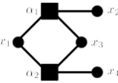
Here we simply explain operations of the (loopy) belief propagation algorithm. First let us consider a pairwise binary model Eq. (1.5) on a tree in Figure 1.2. We write Ψij(xi, xj) =
Figure 1.2: A tree.
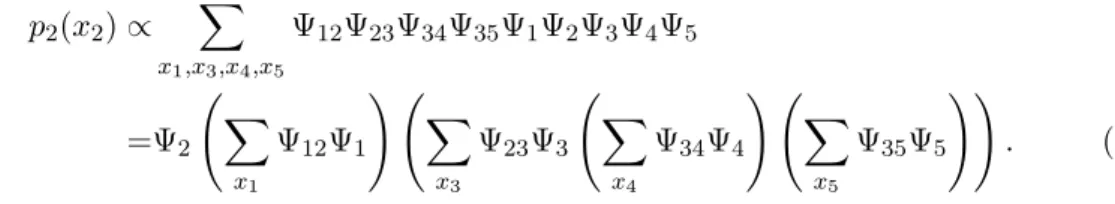
exp(Jijxixj) and Ψi(xi) = exp(hixi). Then a marginal distribution p2 is given by p2(x2)∝ X
x1,x3,x4,x5
Ψ12Ψ23Ψ34Ψ35Ψ1Ψ2Ψ3Ψ4Ψ5
=Ψ2 Ã
X
x1
Ψ12Ψ1
! Ã X
x3
Ψ23Ψ3 Ã
X
x4
Ψ34Ψ4
! Ã X
x5
Ψ35Ψ5
!!
. (1.9)
In the above equality, we used the commutativity and the distributive law of the sum and the product. If we define messages by
m1→2(x2) :=X
x1
Ψ12(x1, x2)Ψ1(x1) m4→3(x3) :=X
x4
Ψ34(x3, x4)Ψ4(x4) m5→3(x3) :=X
x5
Ψ35(x3, x5)Ψ5(x5)
and
m3→2(x2) :=X
x3
Ψ23(x2, x3)Ψ3(x3)m4→3(x3)m5→3(x3), Eq. (1.9) becomes
p2(x2)∝ Ψ2(x2)m1→2(x2)m3→2(x2). The partition function is also computed using messages;
Z =X
x2
Ψ2(x2)m1→2(x2)m3→2(x2). (1.10)
Obviously, this method is applicable to arbitrary trees; it is called the belief propagation
algorithm. More formally, define messages for all directed edges (j → i) inductively by mj→i(xi) =X
xj
Ψi(xi)Ψij(xi, xj) Y
k∈Njri
mk→j(xj), (1.11)
where Nj is the neighboring vertices of j. Since we are considering a tree, this equation uniquely determines the messages. The marginal distribution of xi and the partition func- tion are given by
pi(xi)∝ Ψi(xi) Y
j∈Ni
mj→i(xi), (1.12)
Z =X
xi
Ψi(xi) Y
j∈Ni
mj→i(xi). (1.13)
These computations requires only O(|E|) steps. Therefore, the marginals and the partition function of a graphical model associated with a tree can be computed in practical time.
Secondly, let us consider the case that the underlying graph is not a tree. In this case, Eq. (1.11) does not determine the messages explicitly. However, we can solve Eq. (1.11) and obtain a set of messages as a solution. Though this equation has possibly many solutions, we take one solution that is obtained by iterative applications of Eq. (1.11). In other word, we use the equation as an update rule of the messages and find a fixed point. Then, at a fixed point, the approximation of a marginal distribution is given by Eq. (1.12). This method is called the loopy belief propagation. The approximation for the partition function is slightly involved; we will explain it in the next subsection.
1.2.2 Variational formulation of LBP
At first sight, the loopy belief propagation looks groundless because it is just a diversion of the belief propagation, which is guaranteed to work only on trees. However, Yedidia et al [135] have shown the equivalence to the Bethe approximation, making the algorithm on a concrete theoretical ground. More precisely, the LBP algorithm is formulated as a variational problem of the Bethe free energy function.
Again, we explain the variational formulation in the case of the model Eq. (1.5). Let b ={bij, bi}ij∈E,i∈V be a set of pseudomarginals, i.e., functions satisfying Px
ibij(xi, xj) =
bj(xj), Pxi,xjbij(xi, xj) = 1 and bij(xi, xj) ≥ 0. The Bethe free energy function is defined
on this set by F (b) =− X
ij∈E
X
xi,xj
bij(xi, xj) log Ψij(xi, xj)−X
i∈V
X
xi
bi(xi) log Ψi(xi)
+ X
ij∈E
X
xi,xj
bij(xi, xj) log bij(xi, xj) +X
i∈V
(1− di)X
xi
bi(xi) log bi(xi), (1.14)
where di = |Ni| is the number of neighboring vertices of i. Note that this function is not convex in general and possibly has multiple minima. The result of [135] says that the stationary points of this problem correspond to the solutions of the loopy belief propagation. (The positive definiteness of the Hessian of the Bethe free energy function will be discussed in Section 4.3. The uniqueness of LBP fixed point will be discussed in Chapter 5.)
Similar to the case of the mean field approximation, this variational problem can be viewed as a KL-divergence minimization [136], i.e., if we take (not necessarily normalized) distribution
q(x) =Y
ij
bij(xi, xj) bi(xi)bj(xj)
Y
i∈V
bi(xi), (1.15)
then D(q||p) ≈ F (b) + log Z. Since we are expecting the KL-divergence is nearly zero at a stationary point b∗, this relation motivates to define the approximation ZB of the partition function Z by
log ZB :=−F (b∗). (1.16)
1.2.3 Applications of LBP algorithm
Since LBP is essentially equivalent to the Bethe approximation, its application dates back to the 1930’s when Bethe invented the Bethe approximation [15]. In 1993, Berrou et al [13], proposed a novel method of error correcting codes and found its excellent performance. This algorithm was later found to be a special case of LBP by McEliece and Cheng [81]. This discovery made the LBP algorithm popular. Soon after that, the LBP algorithm is success- fully applied to other problems including computer vision problems and medical diagnosis [39, 89]. Since then, scope of the application of the LBP algorithm is expanding. For exam- ple, LBP has many application in image processing such as super-resolution [19], estimation of human pose [59] and image reconstruction [117]. Gaussian loopy belief propagation is also used for solving linear equations [105] and linear programming [16].
1.2.4 Past researches and our approaches
In this subsection, we review the past theoretical researches on LBP, motivating further analysis. A large number of researches have been performed by many researchers to make better understanding of the LBP algorithm.
Behavior of LBP is complicated in general in accordance with non-convexity of the Bethe free energy. LBP has possibly many fixed points, and furthermore, may not converge. For discrete variable models, because of the lower-boundedness of Bethe free energy, at least one fixed point is guaranteed to exist [136]. Fixed points are not necessarily unique in general, but for trees and one-cycle graphs, the fixed point is guaranteed to be unique [128]. This fact motivates analysis on classes of graphs that have a unique fixed point. Each LBP fixed point is a solution of a nonlinear equation associated with the graph. Therefore, the problem of the uniqueness of LBP is the uniqueness of the solution of this equation. In the next section we discuss the history of this kind of problems in mathematics to show an alternative origin of our research.
As mentioned above, the algorithm does not necessarily converge and often shows os- cillatory behaviors. Concerning the discrete variable model, Mooij [87] gives a sufficient condition for convergence in terms of the spectral radius of a certain matrix related to the graph geometry. This matrix is the same as the matrix that appears in the (multivariate) Ihara-graph zeta function [110]. The graph zeta function is a popular characteristic of a graph; it is originally introduced by Ihara [60]. Mooij’s result has not been considered from the view of the graph zeta function nor graph geometry. In this thesis, developing a new formula, we show a partial answer why this matrix appears in the sufficient condition of convergence.
The approximation performance has been also a central issue for understanding empirical success of LBP. Since the approximation of marginals for a discrete model is also an NP-hard problem [31], it seems difficult to obtain high quality error bounds. Therefore, rather than rigorous bounds, we need to develop intuitive understanding of errors. For binary models, Chertkov and Chernyak [24, 25] derived an expansion called loop series that expresses the ratio of Z and its Bethe approximation in a finite sum labeled by a set of subgraphs called generalized loops. We also derive an expansion of marginals in a similar manner. An interesting point of the loop series is that the graph geometry explicitly appears in the error expression and non-existence of generalized loop in a tree immediately implies the exactness of the Bethe approximation and LBP. Concerning the error of marginals, Ikeda et al [64, 63]
have derived perturbative analysis of marginals based on the information geometric methods [4]. For Gaussian models, though the problem is not NP-hard, Weiss and Freeman have shown that the approximated means by LBP are exact but not for covariances [129].
For understanding of LBP errors, we follow the loop series approach initiated by Chertkov and Chernyak. One reason is that the full series is easy to handle because it is a finite sum. Though the expansion is limited to binary models, it covers important applications such as error correcting codes.
As discussed in the previous subsection, LBP is interpreted as a minimization problem, where the objective function is the Bethe free energy. Empirically, Yedidia et al [135] found that locally stable fixed points of LBP are local minima of the Bethe free energy function. For discrete models, Heskes [54] has shown that stable fixed points of LBP are local minima of the Bethe free energy function. This fact suggests that LBP finds a locally good stationary point. From a theoretical point of view, this relation suggests that there is a covered relation between the LBP update and the local structure of the Bethe free energy. Analysis of the Bethe free energy itself is also an important issue for understanding of LBP. Pakzad et al [95] have shown that the Bethe free energy is convex if the underlying graph is a tree or one-cycle graph. But for general graphs, (non) convexity of the Bethe free energy has not been comprehensively investigated. As observed from Eq. (1.14), the Hessian (the matrix of second derivatives) of the Bethe free energy does not depend on the given compatibility function, i.e., only determined by the graph geometry.
The variational formulation naturally derives an extension of the LBP algorithm called Generalized Belief Propagation (GBP) that is equivalent to an extension of the Bethe ap- proximation: Kikuchi approximation [135, 72]. Inspired by this result, many modified variational problems have been proposed. For example, Wiegerinck and Heskes [133] have proposed a generalization of the Bethe free energy by introducing tuning parameter in coeffi- cients. This free energy yields fractional belief propagation algorithm. Since these extended variational problems include the variational problem of the Bethe free energy function, it is still important to understand the Bethe free energy as a starting point.
Finally, we summarize our approach to analysis of LBP motivated by past researches. For tree structured graphs, LBP has desirable properties such as the uniqueness of solu- tion, exactness and convergence at finite step. However, as observed in past researches, existence of cycles breaks down such properties. Organizing these fragmented observations, our analysis tries to make comprehensive understanding on the relation between the loopy
belief propagation and graph geometry. Indeed past researches of LBP have not treated
“graph geometry” in a satisfactory manner; few analysis has derived clear relations going beyond tree/not tree classification. Malioutov et al [79] have shown that errors of Gaussian belief propagation are related to walks of the graph and the universal covering tree, but it is limited to the Gaussian case.
1.3 Discrete geometric analysis
In this thesis, we emphasize the discrete geometric viewpoint, which utilizes graph charac- teristics such as graph zeta function and graph polynomials. First, we introduce another mathematical background of this thesis: the interplay between geometry and equation. This viewpoint puts our analysis of LBP in a big stream of mathematics. Then, we discuss what kind of discrete geometry we should consider.
1.3.1 Geometry and Equations
The fixed point equation of the LBP algorithm Eq. (1.11) involves messages. The messages are labeled by the directed edges of the graph and satisfy local relations. Therefore the structure of the equation is much related to the graph. Since it is an equation, it is natural to ask whether there is a solution. And if so, how many are there and what kind of structure do they have? As mentioned in the previous section, if the underlying graph is a tree or one-cycle graph, the uniqueness of the LBP solution is easily shown [99, 128].
Equations that have variables labeled by points in a geometric object often have ap- peared in mathematics and formed a big stream [121]. There are many examples that involve deep relations between the topology of a geometric object and the properties of equations on it such as solvability. In this thesis, we emphasize this aspect of the LBP equation and add a new example of this story.
Here we explain such an interplay by elementary examples. We can start with the following easy observation.
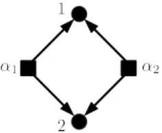
(A)
x = 2x + 3y + z + 3 y =−y + z + 3 z = 2z− 1
(B)
x = 2x + 3y + z + 1 y = x− y + z + 2 + 1 z =−x + y + 2z + 3
(1.17)
Figure 1.3: Graph representation of the equations
One may immediately find the solution of Eq. (A), by computing z, y and x successively. But one may not find a solution of Eq. (B) without paper and a pencil. The difference is easily realized by a graphical representation of these equations (Fig. 1.3). The first one does not include a directed cycle, i.e. a sequence of directed edges that ends the starting point, but the latter has.
This type of difference is understood by the following setting. Consider a linear equa- tion x = Ax + c. If A is an upper diagonal matrix, this equation is solved in order of O(N2) computations by solving one by one. However, for general matrix A, the required computational cost is O(N3) [45]. Existence of directed cycles makes the equation difficult.
Another easy example of interrelation is the Laplace equation;
∇2φ(x) = 0 x∈ Ω; φ(x) = 0 x ∈ ∂Ω. (1.18) Here, the “geometric object” is the region Ω⊂ Rn. This differential equation is characterized by the variational problem of the energy functional:
E[φ] := 1 2
Z
Ωk∇φk
2dx. (1.19)
This characterization reminds us the relation between the LBP fixed point equation and the variational problem of the Bethe free energy functional. In this analogy, the region Ω corresponds to the graph G = (V, E) and the function φ corresponds to messages, or equivalently pseudomarginals, on G. The variation of the energy functional and the Bethe free energy gives equation ∇2φ(x) = 0 and the LBP fixed point equation, respectively. The equation ∇2φ(x) = 0 is local because it is a differential equation. Similarly, the LBP fixed point equation is also local in a sense that it only involves neighboring messages. An
important difference is that the geometric object G is discrete.
The space of solution is much related to the geometry of Ω. For example let n = 2 and D1 ={(x, y)|x2+ y2 < 1} and D2 ={(x, y)|1 < x2+ y2}. If Ω = D1, the only solution is φ = 0 from the maximum principle [2]. But if Ω = D2, there is a nonzero solution
φ(x, y) = ln(x2+ y2).
The Laplace equation can be generalized to be defined on Riemannian manifolds. The spectrum of the Laplace operator is intimately related to the zeta function of the manifold which is defined by a product of prime cycles [114]. Furthermore, there is an analogy between Riemannian manifolds and finite graphs, and the graph zeta function is known as a discrete analogue of the zeta function of Riemannian manifold [1]. The spectrum of a discrete analogue of the Laplacian is investigated by [28].
It is noteworthy that the LBP fixed point equation is a non-linear equation though aforementioned examples are linear equations. Analysis of LBP does not reduce to finite dimensional linear algebra, e.g., eigenvalues and eigenvectors. This fact potentially produces a new aspect of analysis on graphs compared to linear algebraic analysis on graphs [43, 36].
1.3.2 What is the geometry of graphs?
Let us go back to the question: what kind of discrete geometry should we employ to understand LBP and the Bethe approximation? We have to think of graph quantities that are consistent with properties of LBP and the partition function. In other words, if there is some theory that relates the graph geometry and properties of the partition function and LBP, they must share some common properties. Such requirements give hints to our question.
One may ask for a hint of topologist. A graph G = (V, E) is indeed a topological space when each edge is regarded as an interval [0, 1] and they are glued together at vertices. However, the basic topology theory can not treat rich properties of the graph, because it can not distinguish homotopy equivalent spaces and the homotopy class of a graph is only determined by the number of connected components k(G) and the nullity n(G) =
|E| − |V | − k(G). In this sense, graph theory is not in a field of topology but rather a combinatorics [80].
For the computation of the partition function, the nullity is much related to its difficulty.
Let K be the number of states of each variable. We can compute the partition function by Kn(G) sums, because if we cut n(G) edges of G, we obtain a tree. But the partition function on a bouquet graph, i.e. a graph that has one vertex with multiple edges, is easily computed in K steps. Therefore, for the understanding of the computation and the behavior of LBP, we need more detailed information of graph geometry that distinguishes graphs with the same nullity.
Therefore, we should ask for graph theorists. Graph theory has been investigating graph geometry in many senses. There are many graph characteristics, which are invariant with respect to graph isomorphisms [34, 35]. The most famous example is the Tutte polynomial [120], which plays an important role in graph theory, a broad field of mathematics and theoretical computer science. However, this thesis does not discuss the Tutte polynomial because it does not meet criteria discussed below.
In the LBP equation, one observes that vertices of degree two can be eliminated without changing the structure of the equation, because this is just a variable elimination. On the other hand, for the problem of computing the true partition function, one also observes that vertices of degree two can be eliminated with low computational cost keeping the partition function.
The operation of eliminating edges with a vertex of degree one also keeps the problem essentially invariant, i.e., LBP solutions are invariant under the operation and the true partition function does not change up to a trivial factor.
In this thesis, we consider two objects associated with the graph: graph zeta function and Θ polynomial. We use them in a multivariate form; in other words, we define them on (directed) edge-weighted graphs. These quantities are desired properties consistent with the above observations. That is,
1. “invariant” to removal of a vertex of degree one and the connecting edge. 2. “invariant” to erasure of a vertex of degree two.
For the second property, we need to explain more. Assume that there is a vertex j of degree two and its neighbors are i and k. If we have directed edge weights ui→j and uj→k, we can erase the vertex i taking ui→k = uj→iui→j keeping the graph zeta function invariant. A similar result holds for the Θ polynomial though its weights are associated with undirected edges.
The first property immediately implies that these quantities are in some sense trivial if the graph is a tree. This property reminds us that LBP gives the exact result if the graph is a tree.
Indeed, these properties do not uniquely determine the quantities associated to graphs. However, it gives a clue to answer our question: what kind of graph geometry is related to LBP?
1.4 Overview of this thesis
The remainder of the thesis is organized in the following manner. Chapter 2: Preliminaries
This chapter sets up the problem formally, introducing hypergraphs, graphical models and exponential families. The Loopy Belief Propagation (LBP) algorithm is also introduced utilizing the language of the exponential families. Our characterizations of LBP fixed points gives an understanding of the Bethe-zeta formula, as discussed in the first section of Chapter 4.
Part I: Graph zeta in Bethe free energy and loopy belief propagation
The central result of this part is the relation between the Hessian of the Bethe free en- ergy and the multivariate graph zeta function. The multivariate graph zeta function is a computable characteristic of an edge weighted graph because it is represented by the determinant of a matrix indexed by edges.
The focus of this part is mainly an intrinsic nature of the LBP algorithm and the Bethe free energy. Namely, we do not treat the true partition function and the Gibbs free energy. Interrelation of such exact quantities and their Bethe approximations is discussed in the next part.
The contents of this part is an extension of the result in [126] where only pairwise and binary models are discussed.
Chapter 3: Graph zeta function
This chapter develops the graph zeta function and related formulas. First, we introduce our graph zeta function unifying known types of graph zeta functions. Secondly, we show
the Ihara-Bass type determinant formula which plays an essential role in the next chapter. Some basic properties of the univariate zeta function, such as places of the poles, are also discussed.
Chapter 4: Bethe-zeta formula
This chapter presents a new formula, called Bethe-zeta formula, which establishes the re- lation between the Hessian of the Bethe free energy function and the graph zeta function. This formula is the central result in Part I. The proof of the formula is based on the Ihara- Bass type determinant formula and Schur complements of the (inverse) covariance matrices. Demonstrating the utility of this formula, we discuss two applications of this formula. The first one is the analysis of the positive definiteness and convexity of the Bethe free energy function; the second one is the analysis of the stability of the LBP algorithm.
Chapter 5: Uniqueness of LBP fixed point
This chapter develops a new approach to the uniqueness problem of the LBP fixed point. We first establish an index sum formula and combine it with the Bethe-zeta formula. Our main contribution of this chapter is the uniqueness theorem for unattractive (frustrated) models on graphs with nullity two. Though these are toy problems, the analysis exploits the graph zeta function and is theoretically interesting. This chapter only discusses the binary pairwise models but our approach can be basically generalized to multinomial models.
Part II: Loop Series
In this part, focusing on binary models, we analyze the relation between the exact quantity, such as the partition function and marginal distributions, and their Bethe approximations using the loop series technique. The expansion provides graph geometric intuitions of LBP errors.
Chapter 6: Loop series
Loop Series (LS), which is developed by Chertkov and Chernyak [24, 25], is an expansion that expresses the approximation error in a finite sum in terms of a certain class of sub- graphs. The contribution of each term is the product of local contributions, which are easily calculated by the LBP outputs. First we explain the derivation of the LS in our notation,
which is suitable for the graph polynomial treatment in the next chapter. In a special case of the perfect matching problems, we observe that the loop series has a special form and is related to the graph zeta function. We also review some applications of the loop series.
Chapter 7: Graph polynomials from Loop Series
This chapter treats the loop series as a weighted graph characteristics called theta poly- nomial, ΘG(β, γ). Our motivation for this treatment is to “divide the problem in two parts.” The loop series is evaluated in two steps: 1. the computation of β = (βij)ij∈E and γ= (γi)i∈V by an LBP solution; 2. the summation of all subgraph contributions. Since the first step seems difficult, we focus on the second step. If there is an interesting property in the form of the sum, or the Θ-polynomial, the property should be related to the behavior of the error of the partition function approximation.
Though we have not been successful in deriving properties of Θ-polynomial that can be used to derive properties of the Bethe approximation, we show that the graph polynomials θG(β, γ) and ωG(β), which are obtained by specializing ΘG, have interesting properties: deletion-contraction relation. We also discuss partial connections to the Tutte polynomial and the monomer-dimer partition function. We believe that these results give hints for future investigations of Θ-polynomial.
Chapter 8: Conclusion
This chapter concludes this thesis and suggests some future researches.
Appendix
In Appendix A, we summarize useful mathematical formulas, which are used in proofs of this thesis. In Appendix B, we put topics on LBP which are not necessary for the logical thread of this thesis, but helpful for further understandings.
Preliminaries
In this chapter, we introduce objects and methods studied in this thesis. Probability distri- butions that have “local” factorization structures appear in many fields including physics, statistics and engineering. Such distributions are called graphical models. Loopy Belief Propagation (LBP) is an efficient approximation method applicable to inference problems on graphical models. The focus of this thesis is an analysis of this algorithm applied to any graph-structured distributions. We begin in Section 2.1 with elements of hypergraphs as well as graphical models because the associated structures with these graphical models are, precisely speaking, hypergraphs. Section 2.2 introduces the LBP algorithm on the basis of the theory of exponential families. A collection of exponential families, called inference family, is utilized to formulate the algorithm. The Bethe free energy, which gives alter- native language for formulating the approximation by the LBP algorithm, is discussed in Section 2.3, providing characterizations of LBP fixed points.
2.1 Probability distributions with graph structure
Probability distributions that are products of “local” functions appears in a variety of fields, including statistical physics [100, 42], statistics [132], artificial intelligence [99], coding the- ory [81, 78, 40], machine learning [70], and combinatorial optimizations [82]. Typically, such distributions come from system modeling of random variables that only have “local” interactions/constraints. These factorization structures are well visualized by graph repre- sentations, called factor graphs. Furthermore, the structures are cleverly exploited in the algorithm of LBP.
31
Figure 2.1: Hypergraph H. Figure 2.2: Two representations.
We start in Subsection 2.1.1 with an introduction of hypergraphs because factor graphs are indeed hypergraphs. Further theory of hypergraphs is found in [12]. Subsection 2.1.2 formally introduces the factor graph of graphical models with some examples.
2.1.1 Basic definitions of graphs and hypergraphs
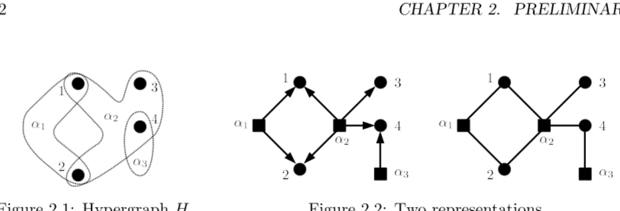
We begin with the definition of (ordinary) graphs. A graph G = (V, E) consists of the vertex set V joined by edges of E. Generalizing the definition of graphs, we define hypergraphs. A hypergraph H = (V, F ) consists of a set of vertices V and a set of hyperedges F . A hyperedge is a non-empty subset of V . Fig. 2.1 illustrates a hypergraph H = ({1, 2, 3}, {α1, α2, α3}), where α1={1, 2}, α2 ={1, 2, 3, 4} and α3={4}.
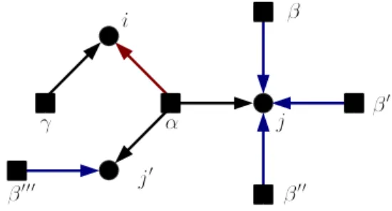
In order to describe the message passing algorithm in Section 2.2.3, it is convenient to identify a relation i ∈ α with a directed edge α → i. The left of Fig. 2.2 illustrates this representation of the above example, where squares represent hyperedges. Therefore, explicitly writing the set of directed edges ~E, a hypergraph H is also denoted by H = (V ∪ F, ~E).
It is also convenient to represent a hypergraph as a bipartite graph. A graph G = (V, E) is bipartite if the vertices are partitioned into two set, say V1 and V2, and all edges join the vertices of V1 and V2. A hypergraph H = (V ∪ F, ~E) is identified with a bipartite graph BH = (V ∪ F, EBH), where EBH is obtained by forgetting the directions of ~E. (See the right of Fig. 2.2.)
For any vertex i ∈ V , the neighbors of i is defined by Ni :={α ∈ F |i ∈ α}. Similarly, for any hyperedge α∈ F , the neighbors of α is defined by Nα := {i ∈ V |i ∈ α} = α. The degrees of i and α are given by di:=|Ni| and dα:=|Nα| = |α|, respectively. A hypergraph H = (V, F ) is called (a, b)-regular if di = a and dα = b for all i ∈ V and α ∈ F . If all the degrees of hyperedges are equal to two, a hypergraph is naturally identified with a graph.
Figure 2.3: Core of hypergraph in Fig. 2.2.
A walk W = (i1, α1, i2, . . . , αn, in+1) of a hypergraph is an alternating sequence of ver- tices and hyperedges that satisfies αk ⊃ {ik, ik+1}, ik6= ik+1 for k = 1, . . . , n. We say that W is a walk from i1 to in+1 and has length n. A walk W is said to be closed if i1 = in+1. A cycle is a closed walk of distinct hyperedges.
A hypergraph H is connected if for every pair of distinct vertices i, j there is a walk from i to j. Obviously, a hypergraph is a disjoint union of connected components. The number of connected components of H is denoted by k(H). The nullity of a hypergraph H is defined by n(H) :=|V | + |F | − | ~E|.
Definition 1. A hypergraph H is a tree if it is connected and has no cycle.
This condition is equivalent to n(H) = 0 and k(H) = 1. Other characterization will be given in Propositions 2.1 and 3.2. Note that this definition of tree is different from hypertree known in graph theory and computer science [104, 47]. For example, the hypergraph in Fig 2.1 is a hypertree though it is not a tree in our definition.
Core of hypergraphs
Here, we discuss the core of hypergraphs, which gives another characterization of trees. The core1 of a hypergraph H = (V, F ), denoted by core(H), is a hypergraph that is obtained by the union of the cycles of H. In other words, core(H) = (V′, F′) is given by F′ = {α ∈ F |α is in some cycles of H} and V′ = {i ∈ V |i is in some cycles of H}. A hypergraph H is said to be a coregraph if H = core(H). See Fig. 2.3 for an example.
Intuitively, the core of a hypergraph is obtained by removing vertices and hyperedges of degree one until there is neither such vertices nor hyperedges. More precisely, the operation for obtaining the core is as follows. First, for H = (V∪F, ~E), find a directed edge (α→ i) ∈
1This term is taken from [109] where the core of graphs is defined. Note that this notion is different from the core in [43].
E that satisfies d~ α = 1 or di = 1. If both of the condition is satisfied, remove α, i and (α→ i). If either of them is satisfied, remove (α→ i) and the degree one vertex/hyperedge.
The following characterization of tree is trivial from the above definitions.
Proposition 2.1. A connected hypergraph H is a tree if and only if core(H) is the empty hypergraph.
2.1.2 Factor graph representation
Our primary interest is probability distributions that have factorization structures repre- sented by hypergraphs.
Definition 2. Let H = (V, F ) be a hypergraph. For each i∈ V , let xi be a variable that takes values inXi. A probability density function p on x = (xi)i∈V is said to be graphically factorized with respect to H if it has the following factorized form
p(x) = 1 Z
Y
α∈F
Ψα(xα), (2.1)
where xα= (xi)i∈α, Z is the normalization constant and Ψαis non-negative valued function called compatibility function. A set of compatibility functions, giving a graphically factorized distribution, is called a graphical model. The associated hypergraph H is called the factor graph of the graphical model.
We often refer to a hypergraph as a factor graph, implicitly assuming that it is associated with some graphical model. For a factor graph, a hyperedge is usually called a factor. Factor graph is explicitly introduced in [77].
Any probability distribution onX =QiXiis trivially graphically factorized with respect to the “one-factor hypergraph,” where the unique factor includes all vertices. It is more informative if the factorization involves factors of small sizes. Our implicit assumption in the subsequent chapters is that for all factors α,Xα=QiXiis small, in sense of cardinality or dimension, enough to be handled by computers.
A Markov Random Field (MRF) is an example that have such a factorization structure. Let G = (V, E) be a graph and X = Qi∈V Xi be a discrete set. A positive probability distribution p of X is said to be a Markov random field on G if it satisfies
p(xi|xV ri) = p(xi|xNi) for all i∈ V. (2.2)