Empirical representations of probability
distributions via kernel mean embeddings
Motonobu Kanagawa
Doctor of Philosophy
Department of Statistical Science
School of Multidisciplinary Sciences
SOKENDAI (The Graduate University for
Advanced Studies)
Empirical representations of probability distributions via
kernel mean embeddings
a dissertation
submitted to the faculty of
the school of multidisciplinary sciences
the department of statistical science
the graduate university for advanced studies
by
Motonobu Kanagawa
in partial fulfillment of the requirements
for the degree of
doctor of philosophy
Kenji Fukumizu, Advisor
March 2016
⃝ Motonobu Kanagawa 2016c
Acknowledgements
I am grateful to all people whose have supported me in the process of my Ph.D. course. First and foremost, I would like to express my gratitude to Prof. Kenji Fuku- mizu for being my supervisor since I came to the Institute of Statistical Mathematics as an intern. I would like to thank Prof. Satoshi Kuriki, Prof. Daichi Mochihashi, Prof. Ryo Yoshida, and Prof. Taiji Suzuki for being committee members and for their helpful comments, and Prof. Arthur Gretton and Prof. Yu Nishiyama for being collaborators on the works that become a basis of this thesis. I am also grateful to the members of the Fukumizu laboratory and the SML center, and students and professors of ISM.
Finally, I would like to thank my family for their warm supports.
i
Abstract
How to represent probability distributions is a fundamental issue in statistical meth- ods, as this determines all the subsequent estimation procedures. In this thesis, we focus on the approach using positive definite kernels and reproducing kernel Hilbert spaces (RKHS), namely the framework of kernel mean embeddings. In this frame- work, any probability distribution is represented as an element in an RKHS, which is called the kernel mean. Since each kernel mean contains all the information about the embedded distribution, statistical inference can be conducted by estimating the kernel means of distributions which one is interested in. In general, a finite sample estimate of a kernel mean is given as a weighted sum of feature vectors. Therefore an empirical kernel mean is expressed by a weighted sample, and thus it is similar to an empirical distribution.
In this thesis, we investigate this similarity between empirical kernel means and empirical distributions, and show that empirical kernel means can be treated as em- pirical distributions; this enables us to incorporate Monte Carlo methods into the framework of kernel mean embeddings. We first prove that a sampling method can be applied to empirical kernel means, as is commonly done to empirical distributions in the field of Monte Carlo methods. Based on this theoretical result, we develop a novel method for filtering in a state-space model, which effectively combines the sampling method and a nonparametric learning approach of kernel mean embeddings. We also prove that empirical kernel means can be used for estimating expectations of functions of a broad class, similarly to empirical distributions.
ii
Contents
List of Tables v
List of Figures vi
1 Introduction 1
1.1 Representations of probability distributions . . . 1
1.2 Kernel mean embeddings of distributions . . . 3
1.3 Empirical distributions and Monte Carlo methods . . . 5
1.4 Contributions . . . 6
2 Kernel mean embeddings of distributions 10 2.1 Positive definite kernels and reproducing kernel Hilbert spaces . . . . 10
2.2 Kernel means . . . 12
2.3 Characteristic kernels and metrics on distributions . . . 13
2.4 Estimation of kernel means . . . 14
2.5 Kernel mean embeddings of conditional distributions . . . 15
2.5.1 Conditional mean embeddings . . . 15
2.5.2 Kernel Bayes’ Rule (KBR) . . . 16
2.6 Properties of weight sample estimators . . . 17
2.7 Kernel Herding . . . 18
3 Sampling and resampling with kernel mean embeddings 20 3.1 Sampling algorithm . . . 21
3.2 Resampling algorithm . . . 23
3.3 Role of resampling . . . 24
3.4 Convergence rates for resampling . . . 26
3.5 Experiments . . . 29
3.6 Proofs . . . 35
3.6.1 Proof of Theorem 1 . . . 35
3.6.2 Proof of Theorem 2 . . . 38
iii
Contents iv
4 Kernel Monte Carlo Filter 44
4.1 Related work . . . 46
4.2 Proposed method . . . 47
4.2.1 Notation and problem setup . . . 47
4.2.2 Algorithm . . . 48
4.2.3 Discussion . . . 51
4.2.4 Estimation of posterior statistics . . . 53
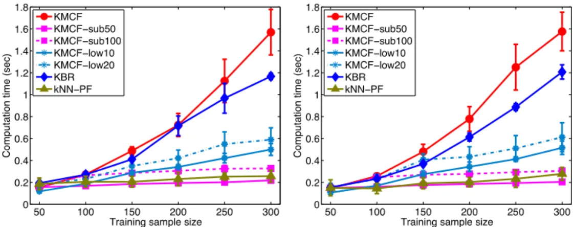
4.3 Acceleration methods . . . 56
4.3.1 Low rank approximation of kernel matrices . . . 56
4.3.2 Data reduction with Kernel Herding . . . 57
4.4 Theoretical analysis . . . 60
4.5 Experiments . . . 61
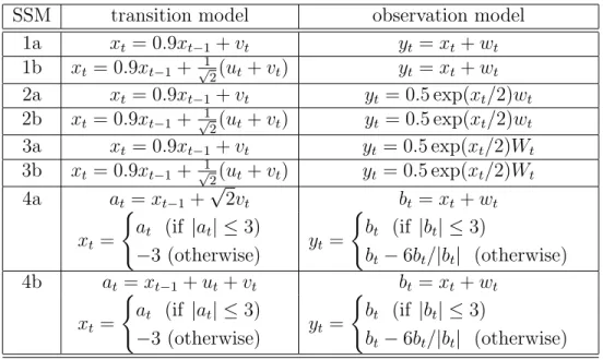
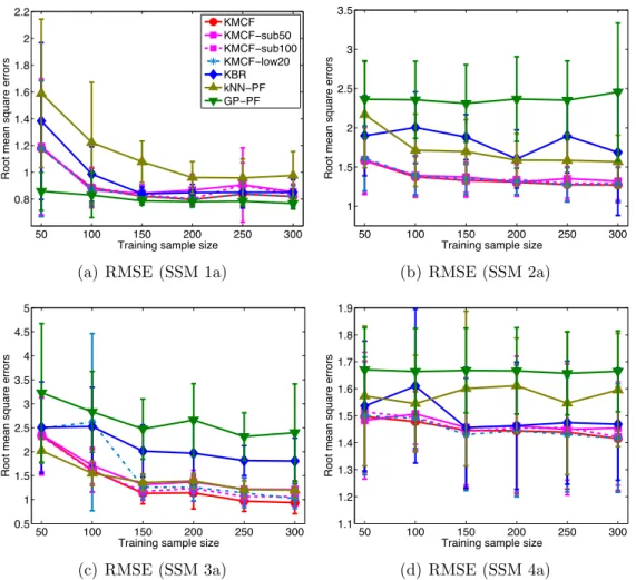
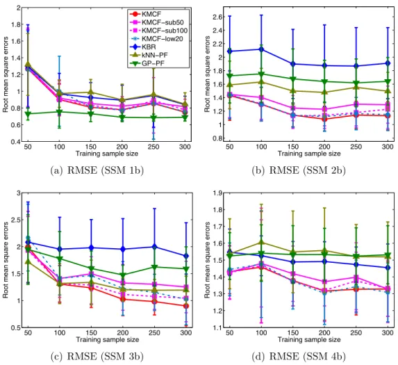
4.5.1 Filtering with synthetic state-space models . . . 62
4.5.2 Vision-based mobile robot localization . . . 67
5 Decoding distributions from empirical kernel means 74 5.1 Related work . . . 76
5.2 Function spaces . . . 78
5.2.1 Sobolev spaces . . . 79
5.2.2 Besov spaces . . . 79
5.2.3 Gaussian reproducing kenrel Hilbert spaces . . . 81
5.3 Main theorem . . . 82
5.3.1 Expectations of infinitely differentiable functions . . . 85
5.3.2 Expectations of indicator functions on cubes . . . 86
5.4 Decoding density functions . . . 87
5.5 Numerical experiments . . . 89
5.6 Proofs . . . 92
5.6.1 Proof of Theorem 4 . . . 92
5.6.2 Proof of Proposition 1 . . . 95
5.6.3 Proof of Corollary 6 . . . 95
5.6.4 Proof of Theorem 5 . . . 96
6 Conclusions and future work 99
References 101
List of Tables
4.1 Notation . . . 48 4.2 State-space models (SSM) for synthetic experiments . . . 63 5.1 Test functions . . . 90
v
List of Figures
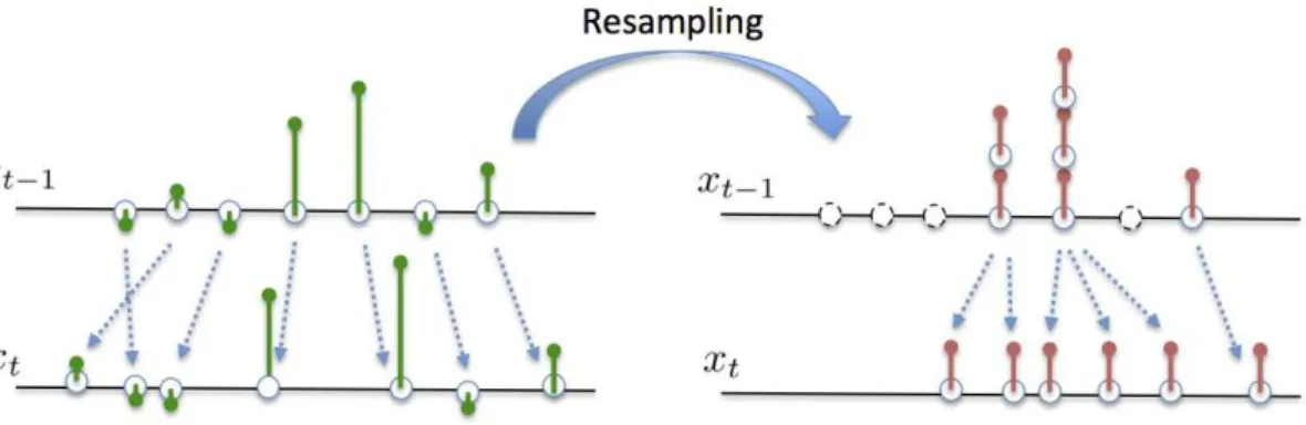
3.1 An illustration of the sampling procedure . . . 25
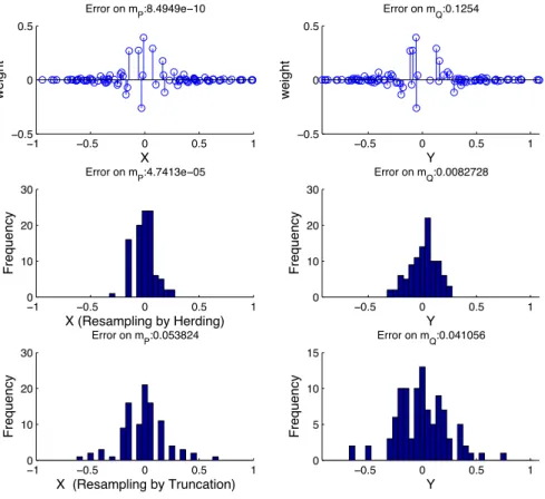
3.2 Results of the experiments from Section 3.5 . . . 33
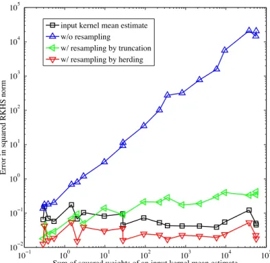
3.3 Results of synthetic experiments for the sampling and resampling pro- cedure in Section 3.5 . . . 34
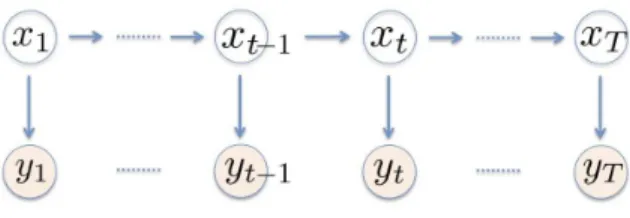
4.1 Graphical representation of a state-space model . . . 45
4.2 One iteration of KMCF . . . 55
4.3 RMSE of the synthetic experiments in Section 4.5.1 . . . 65
4.4 RMSE of synthetic experiments in Section 4.5.1 . . . 66
4.5 Computation time of synthetic experiments in Section 4.5.1 . . . 67
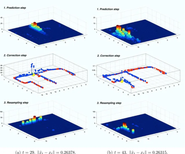
4.6 Demonstration results. . . 70
4.7 Demonstration results . . . 71
4.8 RMSE of the robot localization experiments in Section 4.5.2 . . . 72
4.9 Computation time of the localization experiments in Section 4.5.2 . . 73
5.1 Simulation results for function value expectations with infinitely dif- ferentiable functions. . . 91
5.2 Simulation results for function value expectations with indicator func- tions. . . 91
5.3 Simulation results for function value expectations with polynomial functions. . . 92
vi
Chapter 1
Introduction
Knowing distributions of samples is the ultimate goal of statistical science. This means that many statistical problems may be cast as the problem of estimating unknown distributions.
For instance, let us consider the two sample problem, where one is given inde- pendent samples from two distributions, and the task is to test the homogeneity of these distributions. This can be done by first estimating the two distributions, and then comparing the resulting distribution estimates. Similarly, the problem of mea- suring and testing dependency between two random variables can be seen as that of distribution estimation. This is because statistical dependency is measured by the discrepancy between the joint distribution of the two random variables and the prod- uct distribution of their marginals. Therefore the dependency can be estimated by estimating and comparing these two distributions.
Problems of prediction, rather than those of inference as above, can be also formu- lated as the estimation of unknown distributions. The simplest example is regression, which is essentially the task of estimating the conditional distribution of a response given covariates. Another typical example is the prediction of future observations in time-series data analysis; this is the problem of estimating the distribution of future observations.
1.1 Representations of probability distributions
What is the meaning of “the estimation of probability distributions”? Probability distributions are measures, so one might think of it as the estimation of measures themselves. However, the estimation of measures is not straightforward in practice and may be infeasible. Alternatively, we can consider distribution estimation as the problem of estimating some quantities which are uniquely associated to the distribu- tions of interest; we will call such quantities representations of probability distributions
1
1.1. Representations of probability distributions 2
in this thesis. The following are examples what we consider as probability represen- tations:
Example 1 (Parameters of a parametric family of distributions). Suppose one is interested in distributions belonging to a parametric family of distributions {Pθ : θ ∈ Θ} indexed by finite dimensional vectors θ in a certain set Θ. Since each parameter vector θ is uniquely associated to some distribution Pθ, one can consider these vectors as representations of distributions in the parametric family. Therefore estimating a parameter vector θ amounts to estimating the corresponding distribution Pθ.
Example 2 (Density functions in nonparametric models). Suppose one is interested in a class of distributions that admit density functions of a certain degree of smooth- ness, i.e., a nonparametric density model. In this case, the density functions can be seen as representations of the distributions, since they identify the corresponding distributions in the model.
Example 3 (Characteristic functions). Suppose one is interested in all probability distributions on the Euclidian space Rd. For any distribution P , the characteristic function is defined as the (inverse) Fourier transform of P :
ϕP(w) :=
∫
Rd
e√−1xTwdP (x), w∈ Rd. (1.1) Characteristic functions and distributions are one-to-one (Dudley, 2002, Section 9.5), so one can think of characteristic functions as representations of all distributions on Rd.
For example, consider again the two-sample problem, and suppose there exist some representations of the two distributions. Then testing whether these represen- tations are equal or not yields a solution of the two sample problem, since they are uniquely associated to the two distributions under consideration. Therefore it suffices to estimate those quantities that represent the two distributions.
To make use of such representations in practice, however, one must consider how to estimate them given samples. For parametric models, there are several methods for parameter estimation, ranging from maximum likelihood estimation to Bayesian methods. On the other hand, density functions can be estimated nonparametri- cally, using smoothing methods such as kernel density estimation (Silverman, 1986). Characteristic functions may be estimated as empirical averages of the exponential functions (Feuerverger and Mureika, 1977).
In the estimation of probability representations, there is a tradeoff between the richness of representations and convergence rates. This is the so-called bias-variance tradeoff. For example, parametric models only cover distributions of a finite number
1.2. Kernel mean embeddings of distributions 3
of degrees of freedom, so they are more restrictive than nonparametric models. How- ever, convergence rates are fast and independent of the dimensionality of data. On the other hand, nonparametric models can deal with a wider class of distributions than parametric models, but convergence rates are slow due to the so-called curse of dimensionality: to achieve a certain level of accuracy, the number of samples needs to be exponential to the dimensionality of data (Silverman, 1986).
Characteristic functions enjoy the merits of both parametric and nonparametric approaches: (a) they can represent all distributions on Rd; (b) estimation with an i.i.d. sample can achieve the same convergence rate as those of parametric models (Feuerverger and Mureika, 1977). Nonetheless, the use of empirical characteristic functions in statistical inference and prediction may not be straightforward. For example, comparison of two characteristic functions may be possible by defining dis- tance between them, such as the L2 distance. However, the L2 distance between characteristic functions does not allow an analytic formula with respect to samples, so the computation might require numerical integration1 (Yu, 2004).
1.2 Kernel mean embeddings of distributions
The focus of this thesis is on probability representations based on positive definite ker- nels and associated reproducing kernel Hilbert spaces (RKHS) (Berlinet and Thomas- Agnan, 2004, Chapter 4). This framework has been developed in the machine learning community in the last decades (Smola et al., 2007; Sriperumbudur et al., 2010; Song et al., 2013).
Let X be a measurable space, k : X × X → R be a positive definite kernel and H be the RKHS associated with k (definitions will be given in Chapter 2). The RKHS is a function space consisting of functions on X , properties of which are determined by the kernel k. Then for any probability distribution P on X , its representation in the RKHS H is defined as the expectation of the kernel function with respect to that distribution:
mP := EX∼P[k(·, X)] =
∫
k(·, x)dP (x). (1.2)
This is called the kernel mean of the distribution P . For a rich enough RKHS, it can be shown that probability distributions and kernel means is one-to-one (Sriperumbudur et al., 2010): for any distributions P and Q, mP = mQ holds if and only if P = Q. Therefore kernel means are valid as representations of probability distributions.
1While the L2 distance between empirical characteristic functions may not have an analytic solution, a certain weighted L2 distance does; the resulting distance is known as the energy distance (Sz´ekely and Rizzo, 2013, Proposition 1). The energy distance has a close relationship with kernel mean embeddings discussed in this thesis, as shown by Sejdinovic et al. (2013b).
1.2. Kernel mean embeddings of distributions 4
This approach is akin to representations given by characteristic functions in the following points: (i) the representation of a distribution is given as the expectation of a certain function (i.e. kernel or exponential function) with respect to that dis- tribution; (ii) distribution representations and distributions are one-to-one. In fact, there is a close relationship between these two approaches; one can define a metric on distributions as the RKHS distance between kernel means, and this metric may be written as a weighted L2 distance between characteristic functions (Sriperumbudur et al., 2010).
Compared to existing nonparametric approaches based on densities or character- istic functions, however, kernel mean embeddings have the following advantages:
1. Computation of empirical quantities often allow analytic solutions via simple linear algebraic operations. For instance, the RKHS distance between empirical kernel means can be computed by evaluation of kernel values between samples, which results in computation of kernel matrices. This comes from the so-called the reproducing property of the RKHS.
2. As in other kernel methods in machine learning (Sch¨olkopf and Smola, 2002), empirical performance is not strongly affected by the superficial dimensionality of data. For instance, given an i.i.d. sample of size n from a distribution, the corresponding kernel mean is estimated at a convergence rate Op(n−1/2), which is independent of the dimensionality.
3. The domain of data can be arbitrary, as long as positive definite kernels are defined on that space (e.g. structured data such as images, texts, and graphs). Because of these merits, kernel mean embeddings have been used in a variety of problems in statistics and machine learning. For instance, applications include hy- pothesis testing such as two sample and independence testing (Gretton et al., 2012, 2008; Sejdinovic et al., 2013a), measures of dependency between random variables (Fukumizu et al., 2004, 2009a; Gretton et al., 2005; Fukumizu et al., 2008), state- space models (Song et al., 2009, 2010a; Fukumizu et al., 2013; Zhu et al., 2014; Kana- gawa et al., 2014), belief propagation (Song et al., 2010b, 2011a), graphical model learning (Song et al., 2011b; Song and Dai, 2013; Song et al., 2014), predictive state representations (Boots et al., 2013, 2014), and reinforcement learning (Gr¨unew¨alder et al., 2012b; Nishiyama et al., 2012; van Hoof et al., 2015).
In these applications, a kernel mean mP is estimated as a weighted sum of kernel functions with some weights w1, . . . , wn∈ R and samples X1, . . . , Xn ∈ X :
ˆ mP :=
n
∑
i=1
wik(·, Xi), (1.3)
1.3. Empirical distributions and Monte Carlo methods 5
These weights are typically obtained via linear algebraic operations on kernel matrices, such as regularized matrix inversion (Song et al., 2009, 2013; Fukumizu et al., 2013), singular value decomposition (Song et al., 2010a, 2011b), tensor decomposition (Song et al., 2014), or their combinations. The weights are computed so as to make the estimate (1.3) close to the kernel mean mP, so they can take negative values, and their sum is not necessarily 1.
1.3 Empirical distributions and Monte Carlo meth-
ods
In this thesis, we are interested in the similarity of empirical kernel means (1.3) and empirical distributions. An empirical distribution of a probability distribution P is given as
P =ˆ
n
∑
i=1
wiδXi (1.4)
with some samples X1, . . . , Xn ∈ X and weights w1, . . . , wn ≥ 0, where δx denotes the Dirac measure at x. It is an approximation of the distribution P in that it provides approximations of function value expectations with respect to P (Douc and Moulines, 2008). Namely, let F be a certain set of test functions (e.g. the set of all bounded continuous functions). Then for any f ∈ F, the weighted average ∑ni=1wif (Xi)
should be a good approximation of the expectation EX∼P[f (X)].
Empirical distributions are basis of Monte Carlo methods, as weighted samples are useful for manipulating distributions by simulation. For example, in sequential Monte Carlo (SMC) methods (Doucet et al., 2001), forward probabilities are computed by simulating samples and propagating the associated weights. In Markov chain Monte Carlo (MCMC) methods (Robert and Casella, 2004), new samples are generated conditioned on previously generated samples. The focus of the Monte Carlo methods is not on the estimation unknown distributions: distributions are assumed known in a certain sense; in standard Monte Carlo integration, distributions are known entirely, while in MCMC, distributions are known up to their normalization constants. These methods aims to numerically approximate an intractable integral
∫
f (x)dP (x) (1.5)
for a test function f of a certain class (e.g. polynomials that yield moments). This is done by generating weighted samples{(wi, Xi)}, and computing the weighted sum of
1.4. Contributions 6
function values:
n
∑
i=1
wif (Xi). (1.6)
How to generate the weighted samples depend on the method employed; for the standard Monte Carlo and MCMC, the weights are defined as uniform, while for im- portance sampling and SMC, non-uniform weights are used as each weight represents importance of the associated sample (Liu, 2001).
As mentioned earlier, empirical kernel means (1.3) are similar to empirical distri- butions, as both of them are represented by weighted samples {(wi, Xi)}; the differ- ence is that kernels are used in place of Dirac measures, and the weights may take negative values. Recall that (1.3) is an approximation of the kernel mean mP. From this, it can be easily shown (see Chapter 2) that the weighted sum ∑ni=1wif (Xi) for any function f in the RKHS will be a good approximation of the expectation EX∼P[f (X)] with respect to P . In this sense, the empirical kernel mean can also be seen as an empirical distribution, with test functions being those in the RKHS.
1.4 Contributions
The aim of this thesis is to introduce the following perspective to the theory of kernel mean embeddings: empirical kernel means can be treated as empirical distributions. This is motivated by the similarity between empirical kernel means and empirical distributions mentioned above. The further investigation of this similarity is impor- tant, as it implies that Monte Carlo methods may be combined with empirical kernel means.
Specifically, we ask the following questions, which we address in the chapters written in parentheses:
1. Is it possible to treat empirical kernel means as if they were empirical distribu- tions? More specifically, can we apply operations of Monte Carlo methods to empirical kernel means, as for empirical distributions? (Chapter 3)
2. Can we combine techniques of Monte Carlo methods with learning and inference methods based on kernel mean embeddings? (Chapter 4)
3. Are the test functions for empirical kernel means only restricted to those in the RKHS? In other words, can we estimate expectations of functions outside the RKHS, in the same way as for those in the RKHS? (Chapter 5)
Below we explain these questions along with the contributions of this thesis. After reviewing the theory of kernel mean embeddings in Chapter 2, this thesis proceeds as follows.
1.4. Contributions 7
Chapter 3. This chapter is devoted to theoretical analysis, and discusses applica- bility of a sampling method with an empirical kernel mean. Specifically, we consider a sampling procedure using a conditional distribution, which corresponds to that of a particle filter for computing forward probabilities. We prove that such a sampling method can in fact be used with an empirical kernel mean. More precisely, we prove that this sampling method yields a consistent kernel mean estimator for a forward probability, if the given empirical kernel mean is consistent.
Mainly there are three basic operations on empirical distributions used in Monte Carlo or particle methods (Liu, 2001; Doucet et al., 2001; Doucet and Johansen, 2011):
1. Sampling: generating samples from a conditional distribution, conditioned on samples of an empirical distribution.
2. Importance weighting: updating the weights, by multiplying the importance of each sample to the associated weight.
3. Resampling: sampling from the empirical distribution without replacement, by regarding it as a discrete distribution.
Our analysis reveals that the first operation (sampling) can also be employed with empirical kernel means: this makes it possible to combine the sampling method with existing learning and inference methods of kernel mean embeddings. On the other hand, the other operations are not straightforward to realize with kernel mean embed- dings. This is because these operations make use of the positiveness of the weights of empirical distributions, while those of empirical kernel means can be negative. Our analysis also reveals that resampling can be beneficial to improve the accuracy of the sampling procedure, so it would be desirable to realize it with kernel mean em- beddings. To this end, we propose a novel resampling algorithm based on the Kerne Herding algorithm by Chen et al. (2010). We also provide detailed theoretical analysis of this method, and explain its mechanism.
Chapter 4. In this chapter, we demonstrate how the above procedures can be combined with existing methods of kernel mean embeddings. Specifically, we develop a novel filtering method for state-space models, which we call Kernel Monte Carlo Filter (KMCF).
The proposed method is a combination of the sampling and resampling meth- ods in Chapter 3 and Kernel Bayes Rule by Fukumizu et al. (2013). This filtering method focuses on the setting where the observation model is to be learned from state-observation examples, while the state-transition model is known and sampling is possible. We make use of the sampling and resampling procedures to handle the
1.4. Contributions 8
state-transition model, while using the Kernel Bayes’ Rule to learn the observation model.
This setting is useful in applications where the state variable are defined quantities that are very different from observations. We demonstrate our method in synthetic and real data experiments, which include the challenging problem of vision-based robot localization in robotics.
Chapter 5. In this chapter, we conduct theoretical analysis to investigate whether the weighted sum (1.6) becomes a consistent estimator of the function value expec- tation (1.5) when the test function does not belong to the RKHS. This question is motivated by conceptual and practical reasons. Conceptually, a consistent kernel mean estimator should provide all the information about the distribution P , since the kernel mean mP uniquely identifies this distribution. The practical reason is that RKHSs of widely used kernels (e.g. Gaussian) often do not contain important functions for statistical inference. For example, polynomial functions and indicator functions are not contained in the Gaussian RKHS: expectations of these provide moments and confidence intervals, respectively. This means that it is not guaranteed whether these quantities can be estimated by a consistent kernel mean estimator.
By technical reasons, we focus on kernel mean embeddings using the Gaussian kernel and its RKHS. We prove that in this case, expectations of functions in the Besov space can be estimated with a consistent kernel mean estimator. The Besov space is a generalization of the Sobolev space, and consists of functions with a certain degree of smoothness. It contains functions which are less smooth than those in the Gaussian RKHS. Therefore our results guarantee that the weighted sum (1.6) can be consistent for functions having a certain degree of smoothness, even when these functions do not belong to the Gaussian RKHS. As a corollary, we show that the moments and probably masses on cubes can be estimated with a consistent kernel mean estimator. This result is practically important, as it shows that these important quantities can in fact be estimated with kernel mean embeddings. Finally, we also show that the density can be estimated from a consistent kernel mean estimator. This result is useful in applications where the information of densities is important (e.g., MAP estimation in Bayesian inference).
Chapter 3 and Chapter 4 are based on the following journal and conference papers:
• Kanagawa, M., Nishiyama, Y., Gretton, A., and Fukumizu, K. (2016). Filter- ing with State-Observation Examples via Kernel Monte Carlo Filter. Neural Computation, volume 28, issue 2, pages 382–444.
• Kanagawa, M., Nishiyama, Y., Gretton, A., and Fukumizu, K. (2014). Monte Carlo filtering using kernel embedding of distributions. In Proceedings of the
1.4. Contributions 9
28th AAAI Conference on Artificial Intelligence (AAAI-14), pages 1897–1903. Chapter 5 is based on the following conference paper:
• Kanagawa, M. and Fukumizu, K. (2014). Recovering distributions from Gaus- sian RKHS embeddings. In Proceedings of the 17th International Conference on Artificial Intelligence and Statistics (AISTATS 2014), pages 457–465.
Chapter 2
Kernel mean embeddings of
distributions
In this chapter, we review the framework of kernel mean embeddings.
2.1 Positive definite kernels and reproducing ker-
nel Hilbert spaces
We begin by introducing positive definite kernels and reproducing kernel Hilbert spaces (RKHS), details of which can be found in Sch¨olkopf and Smola (2002); Berlinet and Thomas-Agnan (2004); Steinwart and Christmann (2008).
LetX be a set, and k : X ×X → R be a positive definite (p.d.) kernel: a symmetric kernel k :X × X → R is called positive definite, if for all n ∈ N, c1, . . . , cn ∈ R, and X1, . . . , Xn∈ X , we have
n
∑
i=1 n
∑
j=1
cicjk(Xi, Xj)≥ 0.
Any positive definite kernel is uniquely associated with a Reproducing Kernel Hilbert Space (RKHS) (Aronszajn, 1950). Let H be the RKHS associated with k. The RKHS H is a Hilbert space of functions on X , which satisfies the following important properties:
1. (feature vector): k(·, x) ∈ H for all x ∈ X .
2. (reproducing property): f (x) =⟨f, k(·, x)⟩H for all f ∈ H and x ∈ X , where ⟨·, ·⟩H denotes the inner product equipped with H, and k(·, x) is a function with x fixed.
10
2.1. Positive definite kernels and reproducing kernel Hilbert spaces11
The reproducing property is why the Hilbert H is called the reproducing kernel Hilbert space. Combined with the first property, it implies
k(x, x′) =⟨k(·, x), k(·, x′)⟩H, ∀x, x′ ∈ X . (2.1) Namely, k(x, x′) implicitly computes the inner product between the functions k(·, x) and k(·, x′). Therefore k(·, x) can be seen as an implicit representation of x in H. In fact, the RKHS is often high-dimensional (or even infinite dimensional), and thus the function k(·, x) provides a high-dimensional representation of the data. Therefore k(·, x) is called the feature vector of x, and H the feature space.
It is also well-known (Aronszajn, 1950) that the subspace spanned by the feature vectors {k(·, x)|x ∈ X } is dense in H. This means that any function f in H can be written as the limit of functions of the form fn:=∑ni=1cik(·, Xi), where c1, . . . , cn∈ R
and X1, . . . , Xn∈ X .
For example, positive definite kernels on the Euclidian spaceX = Rdinclude Gaus- sian kernel k(x, x′) = exp(−∥x − x′∥22/2σ2) and Laplace kernel k(x, x′) = exp(−∥x − x∥1/σ), where σ > 0 and ∥ · ∥1 denotes the ℓ1 norm. Notably, kernel methods allow X to be a set of structured data, such as images, texts or graphs. In fact, there exist various positive definite kernels developed for such structured data (Hofmann et al., 2008). Note that the notion of positive definite kernels is different from smoothing kernels in kernel density estimation (Silverman, 1986): a smoothing kernel does not necessarily define an RKHS.
In machine learning, positive definite kernels and RKHSs have been widely used for constructing nonlinear learning methods from the corresponding linear ones (Sch¨olkopf and Smola, 2002; Hofmann et al., 2008). This can be done by representing each data x∈ X as a feature vector k(·, x) in the RKHS H, and defining a linear method in this RKHS. Then the resulting learning methods will be nonlinear to the original data. Significantly, such feature vectors, which can be infinite dimensional, need never be computed explicitly. This is because (i) the constructed linear method in the RKHS can be written in terms of the inner-product between feature vectors, and (ii) such inner-products can be computed by just evaluating kernel values between samples, thanks to the property (2.1). Popular examples of nonlinear methods constructed in this way include support vector machines (Vapnik, 1998; Steinwart and Christmann, 2008), kernel PCA (Sch¨olkopf et al., 1998), and kernel CCA (Akaho, 2001; Bach and Jordan, 2002), among others; see also Sch¨olkopf and Smola (2002); Hofmann et al. (2008).
2.2. Kernel means 12
2.2 Kernel means
We now show how to represent probability distributions using positive definite kernels and the associated RKHSs. Let X be a measurable space, k be a measurable kernel on X that is bounded: supx∈Xk(x, x) < ∞, and H be the RKHS of k. Let P be an arbitrary probability distribution on X . Then the representation of P in the RKHS is defined as the mean of the feature vector:
mP :=
∫
k(·, x)dP (x) ∈ H, (2.2)
which is called the kernel mean of P . This is a natural generalization of feature vector representations of individual points to probability distributions (Berlinet and Thomas-Agnan, 2004, Chapter 4). In fact, if the distribution P is the Dirac measure δx at a point x∈ X , then the kernel mean mP becomes the feature vector k(·, x).
Is the kernel mean mP uniquely associated with the distribution P ? In other words, does the kernel mean preserve all information of the embedded distribution? This question is very important for kernel means to be valid representations of dis- tributions. This holds if the kernel k is characteristic: a positive definite kernel k is defined to be characteristic, if the mapping
P → mP ∈ H
is injective (Fukumizu et al., 2004, 2008; Sriperumbudur et al., 2010). This means that the RKHSH is rich enough to distinguish among all distributions. For example, the Gaussian and Laplace kernels defined on Rdare characteristic. We discuss conditions for kernels being characteristic in Section 2.3.
An important property of the kernel mean (2.2) is the following: by the reproduc- ing property, we have
⟨mP, f⟩H =
∫
f (x)dP (x) = EX∼P[f (X)], ∀f ∈ H. (2.3) That is, the expectation of any function in the RKHS can be given by the inner product between the kernel mean and that function.
We can construct learning methods for kernel means, as have been done for feature vectors in standard kernel methods. This results in learning methods on probability distributions (i.e., each input data itself is a probability distribution or an empirical distribution), such as the support measure machines (Muandet et al., 2012) and distribution regression methods (Szab´o et al., 2015; Jitkrittum et al., 2015). These methods have found applications in a variety of fields, such as astronomy (Muandet and Sch¨olkopf, 2013), ecological inference (Flaxman et al., 2015) and natural language
2.3. Characteristic kernels and metrics on distributions 13
processing (Yoshikawa et al., 2014).
2.3 Characteristic kernels and metrics on distribu-
tions
Conditions for kernels to be characteristic have been extensively studied in the litera- ture (Fukumizu et al., 2008, 2009b; Sriperumbudur et al., 2010; Gretton et al., 2012). Here we review these conditions, following Sriperumbudur et al. (2010).
Shift-invariant kernels on Rd. Let k be a shift-invariant kernel on Rd, that is, there is a positive definite function ψ : Rd→ R such that k(x, y) = ψ(x − y). In this case, a necessary and sufficient condition for the kernel being characteristic is known. Namely, the shift invariant kernel k is characteristic, if and only if the support of the Fourier transform of the function ψ is entire Rd(Sriperumbudur et al., 2010, Theorem 9).
Integrally strictly positive definite kernels on general topological spaces. Let X be a topological space. A measurable and bounded kernel on X is defined to be integrally strictly positive definite, if for all finite non-zero signed Borel measure µ onX , we have
∫ ∫
X
k(x, y)dµxdµ(y) > 0.
It is known that an integrally strictly positive definite kernel is characteristic (Sripe- rumbudur et al., 2010, Theorem 7).
Metric on distributions. We can define a metric on distributions using a charac- teristic kernel. That is, we can define the distance between any distributions P and Q as the RKHS distance between their kernel means:
dk(P, Q) :=∥mP − mQ∥H, (2.4)
∥·∥His the norm of the RKHS:∥f∥H :=√⟨f, f⟩Hfor all f ∈ H. It can be easily shown that this satisfies the conditions of a metric: (i) dk(P, P ) = 0 for any distribution P ; (ii) dk(P, Q) ≤ dk(P, R) + dk(R, Q) for any distributions P , Q and R; and (iii) dk(P, Q) = 0 implies P = Q. The first and second conditions are consequences of the use of the distance in a Hilbert space (i.e. the RKHS H). The third condition is due to the characteristic property of the kernel. Relations to other metrics on distributions have been also studied (Sriperumbudur et al., 2010).
2.4. Estimation of kernel means 14
The distance (2.4) is also called the maximum mean discrepancy (MMD) (Gretton et al., 2012). This is because (2.4) can be written as
∥mP − mQ∥H = sup f ∈H:∥f∥H≤1
∫
f (x)dP (x)−
∫
f (x)dQ(x). (2.5) Namely, by computing the kernel distance, we implicitly consider a witness function in the unit ball of the RKHS such that the difference between function value expectations with respect to the two distributions is maximized.
For the kernel distance, there is another characterization in terms of characteristic functions, if the kernel is shift-invariant on Rd. Let ψ : Rd → R be a bounded, continuous positive definite function, such that k(x, y) = ψ(x−y). Then by Bochner’s theorem, there is a finite nonnegative measure Λ on Rd, such that ψ is given as the Fourier transform of Λ:
ψ(x) =
∫
e−√−1xTwdΛ(w), x∈ Rd. (2.6) Then we have
∥mP − mQ∥H =
√
∫
|ϕP(w)− ϕQ(w)|2dΛ(w), (2.7)
where ϕP and ϕQ denote the characteristic functions of P and Q, respectively (Sripe- rumbudur et al., 2010, Corollary 4). In other words, the kernel distance can be writ- ten as a weighted L2 distance between the characteristic functions, where the weight function is given by the (inverse) Fourier transform the function ψ that induces the kernel. This is very similar to the so-called the energy distance, which uses the weight function defined as ∥w∥1d+1 instead of Λ (Sz´ekely and Rizzo, 2013, Proposition 1).
2.4 Estimation of kernel means
In practice, we want to estimate kernel means from samples. Suppose we are given an i.i.d. sample X1, . . . , Xn from a distribution P . Define an estimator of mP by the empirical mean:
ˆ
mP := 1 n
n
∑
i=1
k(·, Xi). (2.8)
If the kernel k is bounded, then this converges to mP at a rate ∥ ˆmP − mP∥H =
Op(n−1/2) (Smola et al., 2007), where Op denotes the asymptotic order in probability. Note that this rate is independent of the dimensionality of the space X .
2.5. Kernel mean embeddings of conditional distributions 15
This estimate (2.8) can be used to estimate the the kernel distance (2.4) on distri- butions. Suppose we have another sample Y1, . . . , Yn from a distribution Q. Then we can also define an estimate of the kernel mean mQ by ˆmQ := 1n∑ni=1k(·, Yi), which converges at a rate Op(n−1/2). Then the kernel distance (2.4) can be estimated by plugging these kernel mean estimates into (2.4). Thanks to the reproducing property of the kernel, this plugin estimate can be analytically computed by just evaluating the kernel values between the samples:
∥ ˆmP − ˆmQ∥H =√ 1
n2
∑
i,j
k(Xi, Xj)− 2 mn
∑
i,j
k(Xi, Yj) + 1 m2
∑
i,j
k(Yi, Yj). (2.9)
This converges to the population quantity (2.4) at a rate O(n−1/2), since the ker- nel mean estimates converge at this rate. For the kernel distance, there also exist statistically or computationally more efficient estimators (Gretton et al., 2012).
2.5 Kernel mean embeddings of conditional distri-
butions
2.5.1 Conditional mean embeddings
We can also define kernel means for conditional distributions (Song et al., 2009; Gr¨unew¨alder et al., 2012a; Song et al., 2013). To show this, letX and Y be measurable spaces, and (X1, Y1), . . . , (Xn, Yn) be an i.i.d. sample onX ×Y with a joint distribution p(x, y)1. Let kX and kY be bounded measurable kernels on X and Y, respectively. Then the kernel mean of the conditional distribution p(y|x) is defined as
mY |x:=
∫
kY(·, y)p(y|x)dy. (2.10)
Different from the previous ones, the conditional kernel mean depends on the input x ∈ X . Therefore it may be seen as a function-valued function. In fact, conditional kernel means can be understood from the viewpoint of function-valued regression (Gr¨unew¨alder et al., 2012a).
As for the kernel distance, the conditional kernel mean (2.10) can be estimated by simple linear algebraic operations using the joint sample {(Xi, Yi)} Let GX = (kX(Xi, Xj)) ∈ Rn×n be the kernel matrix on the sample X1, . . . , Xn. Then we can
1For simplicity of notation, we use the density form to express the joint and conditional distri- butions.
2.5. Kernel mean embeddings of conditional distributions 16
estimate conditional kernel mean (2.10) as
ˆ mY |x :=
n
∑
i=1
wikY(·, Yi). (2.11)
Here the weights w1, . . . , wn∈ R are computed as
(w1, . . . , wn)T = (GX + nλI)−1kX ∈ Rn,
where λ > 0 is a regularization constant and kX := (kX(x, X1), . . . , kX(x, Xn))T ∈ Rn. Note that the weights are a function of the input x ∈ X . To make this estimator consistent, the regularization constant should be decayed to 0 as the sample size increases. It is known that the estimator achieves min-max optimal convergence rates under certain assumptions (Gr¨unew¨alder et al., 2012a).
2.5.2 Kernel Bayes’ Rule (KBR)
As an extension of the conditional kernel means, we can consider kernel means for posterior distributions, taking prior distributions into account. Estimators of such posterior kernel means have been developed, known as the Kernel Bayes’ Rule (KBR). We next explain these concepts.
Let p(x, y) be a joint probability on the product space X × Y that decomposes as p(x, y) = p(y|x)p(x). Let π(x) be a prior distribution on X . Then the conditional probability p(y|x) and the prior π(x) define the posterior distribution by Bayes’ rule;
pπ(x|y) ∝ p(y|x)π(x).
The assumption here is that the conditional probability p(y|x) is unknown. In- stead, we are given an i.i.d. sample (X1, Y1), . . . , (Xn, Yn) from the joint probability p(x, y). We wish to estimate the posterior pπ(x|y) using the sample. KBR achieves this by estimating the kernel mean of pπ(x|y).
Define the kernel means of the prior π(x) and the posterior pπ(x|y): mπ :=
∫
kX(·, x)π(x)dx, mπX|y :=
∫
kX(·, x)pπ(x|y)dx.
KBR also requires that mπbe expressed as a weighted sample. Let ˆmπ :=∑j=1ℓ γjkX(·, Uj) be a sample expression of mπ, where ℓ∈ N, γ1, . . . , γℓ ∈ R and U1, . . . , Uℓ ∈ X . For
example, suppose U1, . . . , Uℓ are i.i.d. drawn from π(x). Then γj = 1/ℓ suffices. Given the joint sample {(Xi, Yi)}ni=1 and the empirical prior mean ˆmπ, KBR esti-
2.6. Properties of weight sample estimators 17 Algorithm 1 Kernel Bayes’ Rule
1: Input: kY, mπ ∈ Rn, GX, GY ∈ Rn×n, ε, δ > 0.
2: Output: w := (w1, . . . , wn)T ∈ Rn.
3: Λ← diag((GX + nεIn)−1mπ)∈ Rn×n.
4: w← ΛGY((ΛGY)2+ δIn)−1ΛkY ∈ Rn.
mates the kernel posterior mean mπX|y as a weighted sum of the feature vectors:
ˆ mπX|y :=
n
∑
i=1
wikX(·, Xi), (2.12)
where the weights w := (w1, . . . , wn)T ∈ Rn are given by Algorithm 1. Here diag(v) for v ∈ Rn denotes a diagonal matrix with diagonal entries v. It takes as input (i) vectors kY = (kY(y, Y1), . . . , kY(y, Yn))T, mπ = ( ˆmπ(X1), . . . , ˆmπ(Xn))T ∈ Rn, where ˆmπ(Xi) = ∑ℓj=1γjkX(Xi, Uj); (ii) kernel matrices GX = (kX(Xi, Xj)), GY = (kY(Yi, Yj)) ∈ Rn×n; and (iii) regularization constants ε, δ > 0. The weight vector w := (w1, . . . , wn)T ∈ Rn is obtained by matrix computations involving two regular- ized matrix inversions. Note that these weights can be negative.
Fukumizu et al. (2013) showed that KBR is a consistent estimator of the kernel posterior mean under certain smoothness assumptions: the estimate (2.12) converges to mπX|y, as the sample size goes to infinity n → ∞ and ˆmπ converges to mπ (with ε, δ → 0 in appropriate speed). For details, see Fukumizu et al. (2013); Song et al. (2013).
2.6 Properties of weight sample estimators
In general, as shown above, a kernel mean mP is estimated as a weighted sum of feature vectors;
ˆ mP =
n
∑
i=1
wik(·, Xi), (2.13)
with samples X1, . . . , Xn ∈ X and (possibly negative) weights w1, . . . , wn ∈ R. Sup- pose ˆmP is close to mP, i.e., ∥ ˆmP − mP∥H is small. Then ˆmP is supposed to have accurate information about P , as mP preserves all the information of P .
How can we decode the information of P from ˆmP? The empirical kernel mean (2.13) has the following property, which is due to the reproducing property of the
2.7. Kernel Herding 18
kernel:
⟨ ˆmP, f⟩H =
n
∑
i=1
wif (Xi), ∀f ∈ H. (2.14) Namely, the weighted average of any function in the RKHS is equal to the inner product between the empirical kernel mean and that function. This is analogous to the property (2.3) of the population kernel mean mP. Let f be any function in H. From these properties (2.3) (2.14), we have
EX∼P[f (X)]−
n
∑
i=1
wif (Xi)
=|⟨mP − ˆmP, f⟩H| ≤ ∥mP − ˆmP∥H∥f∥H, (2.15)
where we used the Cauchy-Schwartz inequality. Therefore the left hand side will be close to 0, if the error ∥mP − ˆmP∥H is small. This shows that the expectation of f can be estimated by the weighted average ∑ni=1wif (Xi). Note that here f is a function in the RKHS, but the same can also be shown for functions outside the RKHS under certain assumptions when the kernel is Gaussian; this is what we will show in Chapter 5. In this way, the estimator of the form (2.13) provides estimators of moments, probability masses on sets and the density function (if this exists).
2.7 Kernel Herding
Finally, we explain the Kernel Herding algorithm (Chen et al., 2010). Different from estimators discussed above, this algorithm assumes that a kernel mean mP is given. It aims at approximating the kernel mean by a finite sample of possibly small size. In other words, the aim is to generate samples x1, x2, . . . , xℓ ∈ X such that the empirical mean ˇmP := 1ℓ∑ℓi=1k(·, xi) is close to the kernel mean mP in the RKHS, i.e., the error ∥mP − ˇmP∥H is small.
The samples generated in this way are useful for numerical integration: for any function f in the RKHS, the empirical average 1ℓ∑ℓi=1f (xi) gives an approximation of the integral ∫ f(x)dP (x), with an error bounded by ∥f∥H∥mP − ˆmP∥H. This
follows from (2.15). Approaches to generate such samples include Quasi Monte Carlo methods; see (Dick et al., 2013).
Kernel Herding is one approach for this purpose. It generates samples x1, . . . , xℓ
deterministically and greedily, by solving the following optimization problems: x1 = arg max
x∈X
mP(x), (2.16)
xℓ= arg max
x∈X
mP(x)−1 ℓ
ℓ−1
∑
i=1
k(x, xi), (ℓ≥ 2) (2.17)
2.7. Kernel Herding 19
where mP(x) denotes the evaluation of mP at x (recall that mP is a function inH). An intuitive interpretation of this procedure can be given if there is a constant R > 0 such that k(x, x) = R for all x ∈ X (e.g., R = 1 if k is Gaussian). Suppose that x1, . . . , xℓ−1 are already calculated. In this case, it can be shown that xℓ in (2.17) is the minimizer of
Eℓ :=
mP −
1 ℓ
ℓ
∑
i=1
k(·, xi) H
. (2.18)
Thus, Kernel Herding performs greedy minimization of the distance between mP and the empirical kernel mean ˇmP = 1ℓ∑ℓi=1k(·, xi).
It can be shown that the error Eℓ of (2.18) decreases at a rate at least O(ℓ−1/2) under the assumption that k is bounded (Bach et al., 2012). In other words, the herding samples x1, . . . , xℓ provide a convergent approximation of mP. In this sense, Kernel Herding can be seen as a (pseudo) sampling method. Note that mP itself can be an empirical kernel mean of the form (2.13). These properties are important for our resampling algorithm developed in Section 3.2.
It should be noted that Eℓ decreases at a faster rate O(ℓ−1) under a certain as- sumption (Chen et al., 2010): this is much faster than the rate of ℓ i.i.d. samples O(ℓ−1/2). Unfortunately, this assumption only holds when H is finite dimensional (Bach et al., 2012), and therefore the fast rate of O(ℓ−1) has not been guaranteed for infinite dimensional cases.
Chapter 3
Sampling and resampling with
kernel mean embeddings
In this chapter, we discuss the use of sampling with empirical kernel means. As we saw in Chapter 2, in general an empirical kernel mean is given as a weighted sum of feature vectors. This expression is similar to that of an empirical distribution, which is given as a weighted sum of delta functions. In Monte Carlo methods, this representation is combined with sampling methods to realize inference in graphical models. One of the most successful applications is particle filters, where sampling is employed to compute forward probabilities. In this chapter we investigate the applicability of this sampling procedure to an empirical kernel mean. Algorithms presented in this chapter serve as building blocks of the filtering method in Chapter 4.
In Section 3.1, we formulate this sampling procedure in terms of empirical kernel means. We present a theoretical justification, and discuss factors that affect the estimation accuracy of sampling. This reveals that the quantity called effective sample size plays an important role. In Section 3.2, we present a resampling algorithm based on Kernel Herding. This algorithm is motivated by the analysis in Section 3.1, and is proposed for the purpose of improving the accuracy of the sampling procedure. In Section 3.3, we explain in more detail the mechanism of resampling. In Section 3.4, we theoretically analyze the proposed resampling algorithm. This analysis presents a novel convergence result of Kernel Herding, which may be of independent interest. In Section 3.5, we conduct toy experiments to empirically confirm the theoretical results. All proofs are presented in Section 3.6.
20
3.1. Sampling algorithm 21
3.1 Sampling algorithm
We begin by introducing the notation. LetX be a measurable space, and P be a prob- ability distribution on X . Let p(·|x) be a conditional distribution on X conditioned on x∈ X . Let Q be a marginal distribution on X defined by Q(B) =∫ p(B|x)dP (x) for all measurable B ⊂ X .1
Let kX be a positive definite kernel onX , and HX be the RKHS associated with kX. Let mP =∫ kX(·, x)dP (x) and mQ = ∫ kX(·, x)dQ(x) be the kernel means of P and Q, respectively. Suppose that we are given an empirical estimate of mP as
ˆ mP :=
n
∑
i=1
wikX(·, Xi), (3.1)
where w1, . . . , wn ∈ R and X1, . . . , Xn ∈ X . Based on this, we wish to estimate the kernel mean mQ.
We consider the following sampling procedure with the conditional distribution: for each sample Xi, we generate a new sample Xi′ with the conditional distribution Xi′ ∼ p(·|Xi). Then we estimate mQ by
ˆ mQ:=
n
∑
i=1
wikX(·, Xi′). (3.2)
The following theorem provides an upper-bound on the error of (3.2), and reveals properties of (3.1) that affect the error of the estimator (3.2). The proof is given in Section 3.6.1.
Theorem 1. Let ˆmP be a fixed estimate of mP given by (3.1). Define a function θ on X × X by θ(x1, x2) = ∫ ∫ kX(x′1, x′2)dp(x′1|x1)dp(x′2|x2),∀x1, x2 ∈ X × X , and assume that θ is included in the tensor RKHS HX ⊗ HX.2 The estimator ˆmQ (3.2)
1We can consider another measurable space Y for the output variable. Namely, p(·|x) can be a conditional distribution onY conditioned on x ∈ X , and Q can be the resulting marginal distribution on Y. Here, however, we restrict ourselves to the setting X = Y for simplicity of notation. Note also that this setting is sufficient for the application to state-space models in Chapter 4.
2The tensor RKHS HX ⊗ HX is the RKHS of a product kernel kX ×X on X × X defined as kX ×X((xa, xb), (xc, xd)) = kX(xa, xc)kX(xb, xd),∀(xa, xb), (xc, xd) ∈ X × X . This space HX⊗ HX consists of smooth functions on X × X , if the kernel kX is smooth (e.g., if kX is Gaussian; see Sec. 4 of Steinwart and Christmann (2008)). In this case, we can interpret this assumption as requiring that θ be smooth as a function onX × X .
The function θ can be written as the inner product between the kernel means of the conditional distributions: θ(x1, x2) =⟨mp(·|x1), mp(·|x2)⟩H
X, where mp(·|x):=∫ kX(·, x
′)dp(x′|x). Therefore the assumption may be further seen as requiring that the map x→ mp(·|x) be smooth. Note that while similar assumptions are common in the literature on kernel mean embeddings (e.g., Theorem 5 of