Non-Circular Motions of the Perseus
Spiral Arm Revealed by VLBI
Astrometry
Doctor of Science
A Ph.D. dissertation presented
by
Nobuyuki, Sakai
Department of Astronomical Science,
School of Physical Science,
The Graduate University for Advanced Studies
March 2014
We aim to reveal three-dimensional (3D) structure and dynamics of the nearby Perseus arm, since uncertainties in previous distance measurements have prevented us to obtain an accurate picture of the Perseus arm in the Milky Way Galaxy. Recently, VLBI astrometry observations regarded as the direct distance measure- ments have routinely achieved a typical parallax accuracy of ± 20 µas with the best accuracy of 5 µas, corresponding to the achievable distance measurements up to 20 kpc with ± 10 % accuracy. Thus, we have been conducting the VLBI astrometry observations to measure trigonometric parallaxes and proper motions of Galactic 22 GHz H2O masers associated with and/or related to the Perseus arm. Combining our VLBI astrometry results with previous ones drastically improves an understanding of the 3D structure and dynamics of the Perseus arm with respect to previous researches based on 1D observations (e.g., line-of-sight velocities).
This Ph.D. thesis consists of three VLBI astrometry results related to the 3D structure and dynamics of the Perseus arm (as summarized in chapters 2, 3, and 4). Introductions of current understandings and issues for the Galactic disk are summarized in chapter 1. Also, we provide an introduction on VLBI astrometry and VERA (VLBI Exploration of Radio Astrometry) with which we have conducted VLBI astrometry in chapter 1.
In chapter 2, we show astrometry results of high-mass star-forming region IRAS 05168+3634 located at galactic longitude (l) of 170.66◦, galactic latitude (b) of
−0.25◦, and a systemic velocity (VLSR) of −15.5 km s−1. The location close to galactic longitude (l) of 180◦has been known as a problematic region where general distance measurement such as the kinematic distance has a significantly large uncertainty. In fact, we obtained a parallactic distance of 1.88+0.21−0.17 kpc for the source, which is significantly smaller than the previous distance estimate of 6 kpc, which was based on the kinematic distance. Our distance measurement places the source in the Perseus arm, rather the Outer arm. In addition, the accurate distance
i
the source. Combining our astrometry results with the systemic velocity provides the full-space (3D) motion and location of the Perseus arm with which the source is associated. As a result, we obtained peculiar (non-circular) motions of (U , V ) = (8 ± 2, −13 ± 6) km s−1 for the source, assuming a flat rotation curve model with Θ(R) = Θ0 = 240 km s−1. Note that the direction of the peculiar motion is toward the Galactic center (U ) and Galactic rotation (V ), respectively. Our results reveal the 3D structure and motion of the Perseus arm toward the direction of galactic longitude (l) ∼ 170◦ for the first time.
In chapter 3, we present the first measurement of the absolute proper motions of IRAS 00259+5625 (l = 123.07◦, b = −6.31◦, and VLSR= −38.3 km s−1). The source has been known to interact with large-scale star-formation activities around the Perseus arm, since the source is associated with the HI loop called the “NGC281 superbubble”, which extends from the Galactic plane toward negative galactic latitude over ∼ 300 pc. The proper motion components measured with VERA are (µαcosδ, µδ) = (−2.48 ± 0.32, −2.85 ± 0.65) mas yr−1, converted into (µlcosb, µb) = (−2.72 ± 0.32, −2.62 ± 0.65) mas yr−1 in the Galactic coordinates. The measured proper motion perpendicular to the Galactic plane (µb) shows vertical motion away from the Galactic plane at a significance of about ∼4-σ. As for the distance of the source, we obtained a marginal result of 2.4+1.0−0.6 kpc with VERA observations in which the source showed rapid luminosity variation. Using the distance, the vertical motion can be converted into vb = −17.9 ± 12.2 km s−1. The tendency of the large vertical motion is consistent with the previous VLBI results for NGC 281 associated with the same superbubble. Thus, our VLBI results confirm the superbubble expansion whose origin is believed to be star-formation activities (e.g., sequential supernova explosions) in the Perseus arm.
In chapter 4, to confirm the prediction of the density-wave theory in which directions of the systematic peculiar motions (as shown in chapter 2) are changed inversely in inner and outer co-rotation (CR) radii (e.g., Mel’nik et al. 1999), we measured parallax and proper motions of massive star-forming region IRAS 07427- 2400 (l = 240.32◦, b = 0.07◦, and VLSR= 68.0 km s−1) with VERA. The measured
ii
the Perseus arm beyond l ∼ 189◦ in VLBI astrometry. Combining our distance measurement with previous astrometry results shows that the pitch angle (i) of the Perseus arm is a constant between 94.60◦ ≤ l ≤ 240.32◦, being i = 17.7◦ ± 1.8◦, while the pitch angle is changed to i = 11.5◦ ± 1.3◦ in 43.17◦ ≤ l ≤ 240.32◦. This suggests that bifurcation or spur is occurred in 43.17 ◦ ≤ l ≤ 94.60◦ for the Perseus arm, although more astrometry results should be required to confirm the difference of the pitch angle. As for the peculiar motions, we obtained (U , V ) = (−9 ± 8, −3 ± 6) km s−1, which is marginally consistent with the prediction of the density-wave theory with an 1-σ significance in U component.
As an overall discussion of this Ph.D. thesis, we compiled our astrometry re- sults with previous ones to compare between the observations and an analytic gas dynamics model provided by Pinol-Ferrer et al. (2012) and (2014). We used the least-squares method to choose the best model in the comparison.
As a result, we derived our best model with the following parameters: m = 4 (number of arms), i = 11.5◦ (the pitch angle), Rref = 11.0 ± 0.1 kpc (reference position of spiral potential toward the Sun from the Galactic center),√Ψm = 16
± 1 km s−1 (amplitude of the potential), and Ωp = 17.0 ± 0.5 km s−1 kpc−1 (pattern speed of the potential). In the model, gas-dense region appears in front of the reference position (at R < Rref), which is consistent with the galactic shock proposed by Fujimoto (1968) and Roberts (1969). Also, the modeled gas spiral arm traces the VLBI sources in the Perseus arm well. In addition, the model with m = 4 and Ωp = 17.0 ± 0.5 km s−1 kpc−1 locates the inner Lindblad resonance (ILR) to be ∼ 9 kpc. We confirmed that peculiar motions obtained by VLBI observations were actually maximized around R ∼ 9 kpc. The same tendency was also reported by Quillen et al. (2005), who showed an ILR of 8.2+0.3−0.4 kpc with Ωp = 19.0 ± 0.9 km s−1 kpc−1, which was based on stellar peculiar motions around the solar neighborhood. We succeeded the direct comparison between the 3D observations and a model based on the density-wave theory for the first time, and we revealed that the 3D structure and motion over kpc scales of the Perseus arm can be explained by the model.
iii
tions) to choose the best model for understanding the 3D structure and dynamics of the Milky Way Galaxy more accurately, since several models have predicted different natures and evolutions of the Milky Way Galaxy. In the next decade, GAIA satellite will provide us stellar astrometry results with similar position ac- curacy of the VLBI astrometry. The stellar astrometry is essential to discriminate the several models (e.g., the density-wave theory or the recurrent and transient spiral), since the stellar component plays a main role in total mass of the Galactic disk. A combination of gas and stellar astrometry results is promising to obtain the most accurate nature of the Perseus arm as well as that of the Milky Way Galaxy in the near future.
iv
1 General Introduction 1
1.1 Disk Properties of The Milky Way Galaxy . . . 1
1.1.1 Overall picture . . . 1
1.1.2 Circular motions in the disk . . . 11
1.1.3 Non-circular motions in the disk . . . 16
1.1.4 Kinematic distance . . . 24
1.2 VLBI Astrometry . . . 27
1.2.1 The principle of VLBI . . . 27
1.2.2 Position Accuracy of Absolute Astrometry . . . 29
1.2.3 Position Accuracy of Relative Astrometry . . . 30
1.2.4 Sensitivity . . . 32
1.2.5 Target: 22 GHz H2O maser . . . 33
1.2.6 VERA project . . . 38
1.3 Aims of This Thesis . . . 43
2 VLBI Astrometry of IRAS 05168+3634 in the Perseus arm 45 2.1 Introduction . . . 46
2.2 Observations and Data reduction . . . 50
2.2.1 VLBI observations with VERA . . . 50
2.2.2 Data Reduction . . . 53
2.3 Results . . . 54
2.3.1 Trigonometric parallax of IRAS 05168+3634 . . . 54
2.3.2 Systematic proper motions of IRAS 05168+3634 . . . 58
2.4 Discussion . . . 59 v
2.4.3 Peculiar Motions: Comparison between the Perseus Arm
and Other Regions . . . 64
2.5 Conclusion . . . 68
3 Absolute proper motion of superbubble IRAS 00259+5625 71 3.1 Introduction . . . 72
3.2 Observations and Data reduction . . . 75
3.2.1 VLBI observations with VERA . . . 75
3.2.2 Data Reduction . . . 78
3.3 Results . . . 80
3.3.1 Marginal trigonometric parallax of IRAS 00259+5625 . . . . 80
3.3.2 Systematic proper motions of IRAS 00259+5625 . . . 84
3.4 Discussion . . . 89
3.4.1 3D motion of IRAS 00259+5625 . . . 89
3.4.2 NGC281 superbubble traced by IRAS 00259+5625, IRAS 00420+5530, and NGC 281 . . . 90
4 VLBI Astrometry of IRAS 07427-2400 in the 3rd Galactic Quad- rant 97 4.1 Brief Introduction . . . 97
4.2 Observations and Data reduction . . . 99
4.2.1 VLBI observations with VERA . . . 99
4.2.2 Data Reduction . . . 102
4.3 Results . . . 103
4.3.1 Trigonometric parallax of IRAS 07427-2400 . . . 103
4.3.2 Systematic proper motions of IRAS 07427-2400 . . . 107
4.4 Discussion . . . 109
4.4.1 3D location of IRAS 07427-2400 . . . 109
4.4.2 3D motion of IRAS 07427-2400 . . . 117
4.4.3 Comparison between observed non-circular motions and an analytic gas dynamics model . . . 121
vi
vii
General Introduction
1.1 Disk Properties of The Milky Way Galaxy
1.1.1 Overall picture
Our Galaxy is especially called as the Milky Way Galaxy, the Galaxy, or our Galaxy. In 1950s, large scale spiral structure in the Galaxy was firstly discovered by 21-cm (HI:neutral hydrogen) radio observations, since radio observations can see through overall the Galactic disk without dust extinction (e.g., Oort, Kerr & Westerhout 1958). Note that existence of disk components (e.g., stars rotating with respect to the Galactic center) was previously suggested by optical (spectroscopic) observations for the Galaxy (e.g., Oort 1922). Figure 1.1 shows the HIdistribution in the Galaxy, which clearly displays dense spiral patterns.
Following this, Georgelin & Georgelin (1976) proposed a model of the Galaxy as a four-arm spiral pattern based on optical (photometry and spectroscopy) and radio observations toward bright ionized (HII) regions (fig. 1.2). According to observations of external spiral galaxies, bright HII regions trace grand design of spiral pattern, therefore their observations (Georgelin & Georgelin 1976) may tell us the spiral pattern of the Galaxy. Note that they used the excitation parameter U to reduce a selection effect due to a distance from the Sun. U is proportional to (SνD2) with a dimension of pc cm−2, where Sν is the radio continuum flux and D is the distance.
1
G. C.
G.C.
3-kpc arm
Figure 1.1: Distribution of neutral hydrogen in the Galactic System (Oort, Kerr & Westerhout 1958). Note that Galactic longitudes labeled in this figure are different from those used in current coordinates system. Arrows show famous feature called as the 3-kpc expanding arm.
As a work succeeding to Georgelin & Georgelin (1976), Russeil (2003) also proposed a four-arm model using optical and radio observations (fig. 1.3). They covered fainter and farther HII regions than Georgelin & Georgelin (1976), and it is complete for the excitation parameter U brighter than 60 pc cm−2.
Dame & Thaddeus (2008) showed counterpart of the expanding 3-kpc arm (e.g., figures 1.1 and 1.3), the far 3-kpc arm, with Galacic longitude versus velocity (l −v) diagram of CO(J=1−0) as shown in fig. 1.4. The l−v diagram is a powerful tool to discriminate structures in blended regions, while early 21 cm surveys were too poor in angular resolution and sensitivity to distinguish the thin, faint lane of the far 3-kpc arm.
Dame & Thaddeus (2011) used again the CO(J=1−0) l − v diagram with a combination of HI (e.g., fig. 1.5) to trace an extension of the Scutum−Centaurus arm in the 1st Galactic quadrant (e.g., 0◦ < l < 90 ◦). They succeeded to trace the extension, referred to as the New arm, with both CO(J=1-0) and HIemissions (see fig. 3 in Dame & Thaddeus 2011). The New arm is located beyond the Outer arm in the 1st Galactic quadrant, and it appears to be symmetric counterpart of
Norma arm Scutum-Crux arm
Perseus arm Sagittarius-Carina arm
Figure 1.2: Four-armed spiral model of our Galaxy traced by bright HII re- gions (Georgelin & Georgelin 1976). Hatched areas correspond to intensity maxima in radio continuum and in neutral hydrogen. The excitation parameter U is proportional to (SνD2), where Sν is the radio continuum flux and D is the distance (see detail in Schraml
& Mezger 1969).
the nearby Perseus arm (e.g., the inset in fig. 1.5).
Around the Galactic center, two independent bar structures have been observed, which are the Galactic bar (also called as the bulge) and the central “long” bar. The Galactic bar, referred to as the COBE/DIRBE bar (Binney et al. 1997), is the triaxial bulge with an aspect ratio of 10:4:3 (length:width:height) (Gerhard 2002). Gerhard (2002) reported a half length of ∼3.1−3.5 kpc and a position angle of 20◦ relative to the Sun-Galactic center line for the COBE/DIRBE bar. The position angle is increasing clockwise. The latter, the central long bar, was first claimed by Hammersley et al. (2000), which conducted star counts with infrared observa- tions. The central long bar is vertically thinner than the COBE/DIRBE bar, and position angle of the central long bar is larger than that of the COBE/DIRBE bar. The Spitzer GLIMPSE (Galactic Legacy Infrared Mid-Plane Survey Extraor- dinaire) surveys observed three regions, the Galactic disk (GLIMPSE I), around the Galactic center including the nuclear bulge (GLIMPSE II), and the central
Perseus arm
Sagittarius-Carina arm Scutum-Crux arm Norma-Cygnus arm
3-kpc arm Bar
Figure 1.3: Four-armed spiral model of our Galaxy traced by HIIregions (Rus- seil 2003). The symbol size is proportional to the excitation param- eter. Long dashed line shows smaller-scale structure called as the local arm. Dashed-dot-dot line represents the bar orientation and length referred from Englmaier & Gerhard (1999). Short dashed line displays difference between a logarithmic spiral model and ob- served HII regions. Solid line may be connected to the 3-kpc arm.
long bar (GLIMPSE 3D) at 3.6, 4.5, 5.8, and 8.0 µm as shown in fig. 1.6. One of the science targets in the GLIMPSE was the Galactic structure. The GLIMPSE surveys have archived over 100 million stars of which about 90% were red giants, and red-clump giants were appeared with a good fraction in the red giants. The red-clump giants have a small range of intrinsic luminosities, meaning that they can be good standard candles to trace the central long bar. Actually GLIMPSE showed that the number of the stars were systematically higher by ∼25% in the north (the 1st Galactic quadrant) than the south (the 4th Galactic quadrant) at
|l| < ∼30◦. This is strong evidence that an asymmetric structure, a central bar, exists in the central region. Benjamin et al. (2005) determined the radius and position angle of the bar with respect to the Sun-Galactic center line using the GLIMPSE data. The resultant radius and position angle were 4.4±0.5 kpc and 44◦ ±10◦, respectively (e.g., fig. 1.8).
As for amplitudes of the spiral arms in the Galaxy, GLIMPSE detected star- count excesses at the tangent of the Scutum-Centaurus arm, while no excesses
Figure 1.4: Galactic longitude−velocity diagram of CO(J=1−0) emission at Galactic longitude b = 0◦ from Bitran et al. (1997): this survey is sampled every 7.5’ at |b| ≤ 1◦ (every 15’ elsewhere) with an 8.8’ beam to a rms sensitivity of 0.14 K in 1.3 km s−1 channels. The dashed lines are linear fits to the inclined, parallel lanes of emission from the near and far 3 kpc arms: v = −53.1+4.16l and v = +56.0+4.08l were determined for the near and far 3 kpc arms, respectively. The insert is the schematic view of the arms over the longitude ranges in which they can be followed clearly in CO.
were detected at the tangent of the Norma and Sagittarius arms (e.g., fig. 1.7). In addition, Drimmel (2000) and Drimmel & Spergel (2001) showed that infrared ex- cesses in stellar emissions were seen at the Scutum-Centaurus and Perseus arms.
Based on the GLIMPSE data with previous researches over a half century (as described above), Churchwell et al. (2009) proposed a grand-design two-armed barred spiral with several secondary arms for the Galaxy (fig. 1.8). In other words, figure 1.8 summarizes our knowledge of structure of the Milky Way Galaxy using currently available data. We itemize important points for figure 1.8:
1. Two bar structures are seen around the Galactic center.
90° 60° 30° 0° 330° 300° 1 5 0
100
50
0
-50
-100
-150
Galactic Longitude Scutum
Tangent
Centaurus Tangent HI
LSR Velocity (km/s)
A
B D
C
270°
Figure 1.5: l − v diagram of CO(J=1−0) color and HI gray (Dame & Thad- deus 2011). Black curve traces the locus of a logarithmic spiral model with a pitch angle of 14.2◦. Note that the model was con- strained to trace tangents of the Scutum−Centaurus arm. The inset is the sketch to understand relation between the l − v di- agram and the Galactic face-on view (⊙ is the Sun’s location). The letters A−D in the both figures are consistent with each other.
2. Distance to the Galactic center of R0 = 8.0 kpc was assumed (Reid 1993). 3. Two grand-design spiral arms are the Perseus and Scutum-Centaurus arms. 4. Other secondary arms are the Sagittarius, Outer, and Near/Far 3-kpc arms.
Based on the above picture, the structure of the Milky Way Galaxy is thought to be relatively simple, since there are clear symmetry structures: e.g., the near/far 3-kpc arms, the grand-design spiral arms (the Scutum−Centaurus and Perseus arms), and existence of the bar structure. The grand-design spiral arms are thought to extend symmetrically from opposite ends of the central long bar (e.g., figures 1.5 and 1.8).
However, the most problematic point in fig. 1.8 was noted by Churchwell et al.
Figure 1.6: Area coverage of the GLIMPSE surveys with dotted and solid lines superimposed on the COBE/DIRBE 4.9 µm image. Note that the solid line areas were observed for tracing the Galactic central bar.
(2009): “The spiral structure is still the most problematic and deserves much more attention from the community.” This problem is due to a difficulty of measuring a distance toward each spiral arm. We will further explain the difficulty in chapter 1.1.4. We also comment on the distance to the Galactic center, R0. This value is essential for understanding the precise structure of the Milky Way Galaxy, since it scales overall size of the Milky Way Galaxy. There still ramains an uncertainty of the distance (R0) due to the difficulty of the distance measurement. To overcome the problems and obtain the most accurate picture of the Milky Way Galaxy, pre- cise distance measurements toward Galactic components are required.
Recently, VLBI (Very Long Baseline Interferometry) technique has allowed us to conduct direct distance measurements (referred to as astrometry) over kpc scales from the Sun. Reid & Honma (2014) summarized current results of the VLBI astrometry. Note that the VLBI astrometry has observed Galactic masers associ- ated with star-forming regions in typically early evolution phases, and therefore it can trace gas kinematics and structure of the Galactic disk. Fig. 1.9 shows ∼100 astrometry results (including unpublished results) superimposed on an artist’s il- lustration of face-on view of the Milky Way Galaxy (same as fig. 1.8). In the next decade, astrometry results would increase up to ∼400−500 maser sources. Combination of the astrometry results with the previous researches (such as fig. 1.8) can bring us the most accurate picture of the Milky Way Galaxy.
Figure 1.7: Star count density as a function of the Galactic longitude (Churchwell et al. 2009). Used bands were J, H, K, and 4.5 µm from below to top curves. Increasing number of the star counts from J band to 4.5 µm clearly shows lower dust extinc- tions with longer wavelengths. Solid line fit to the 4.5-µm counts was based on the exponential disk model. Excesses of the star counts are seen at the tangent of the Scutum-Centaurus arm, while no excesses are seen at the tangents of the Sagittarius and Norma arms.
In this thesis, we will report three VLBI astrometry results, which are related to one of the grand-design spiral arms, the Perseus arm. Detail of our contributions will be explained in later.
Sun
Figure 1.8: Artist’s illustration of grand-design two-armed barred spiral for the Galaxy based on radio, infrared, and visible (optical) observa- tions (Churchwell et al. 2009). This sketch was made by Robert Hurt of the Spitzer Science Center in consultation with Robert Benjamin at the University of Wisconsin-Whitewater. The main arms are the Scutum-Centaurus and Perseus arms, and the sec- ondary arms are the Sagittarius, the Outer, and the Near/Far 3-kpc expanding arms.
Figure 1.9: Current VLBI (Very Long Baseline Interferometry) astrometry results superimposed on an artist’s illustration of face-on view of the Milky Way Galaxy (Reid & Honma 2014). Names with different colors are consistent with corresponding colored dots. Sun’s location is (X, Y) = (0, 8.4) kpc, assumed.
1.1.2 Circular motions in the disk
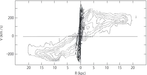
Following the first discovery of galactic rotation by Slipher (1914) using an optical (spectroscopic) observation, there have been similar findings in disk (spi- ral) galaxies with optical/radio observations. Figure 1.10, called as the position- velosity diagram, shows clear symmetry of velocity distribution of an edge-on galaxy NGC 3079 (Irwin & Seaquist 1991; Sofue et al. 2001). This is clear evidence of the galactic rotation, and therefore one can easily expect that the rotation can be also observed in the Milky Way Galaxy, which is thought to be a barred-spiral galaxy as described in previous section.
For the rotation of the Milky Way Galaxy, observational difficulties had pre- vented us to detect the rotation directly in contrast to the external disk galaxies, although suggestions of the rotation had been observed (e.g., Adams & Kohlschut- ter 1914; Adams & Joy 1919; Str¨omberg 1922).
20 15 10 5 0 5 10 15 20
−200 0 200
V (km/s)
R (kpc)
Figure 1.10: The position-velocity diagram aligned with the major axis of NGC 3079, the edge-on galaxy (Sofue et al. 2013). Horizontal axis shows the distance (in kpc) from the center of NGC 3079, and vertical one represents the line-of-sight velocity (in km s−1) at each distance. Dashed and solid contours show HI (Irwin & Seaquist 1991) and CO(J=1-0) (Sofue et al. 2001) line emissions, respectively.
Adams & Kohlschuatter (1914) revealed that most of the high-velocity stars,
which exhibit high velocities with respect to the Sun, showed negative velocities. It means that most of these stars are approaching toward the Sun. Str¨omberg (1922) studied three-dimensional velocity vectors of ∼1,300 stars including the high-velocity stars using radial velocities, proper motions, and (spectroscopic) par- allaxes. He revealed that the high-velocity stars are systematically moving toward opposite direction of the Sun’s motion.
To explain the above observations, Lindblad (1927) made a hypothesis in which galactic components are divided into sub-systems, and each sub-system ro- tates with a different angular speed around the rotation axis perpendicular to the Galactic plane and is originated at the Galactic center. Using the hypothesis, observed line-of-sight (Vr) and tangential (Vt) velocities can be described with a simple geometry (e.g., fig. 1.11) as
Vr =( Θ R −
Θ0
R0 )
R0sinl (1.1)
Vt=( Θ R −
Θ0
R0 )
R0cosl −
Θ
RD. (1.2)
Here Θ the rotation velocity at the galacto-centric distance R, l galactic longitude, D distance from the Sun, and R0 and Θ0 are the Galactic constants.
Oort (1927) derived Vr and Vt especially for solar-neighborhood objects (e.g., D ≪ R0 and D ≪ R) as below:
Vr∼ DA sin2l (1.3)
and
Vt ∼ D(A cos2l + B). (1.4)
Here, A and B are the Oort constants defined as
A ≡ [
−R2 dRd ΘR ]
R0
= 1 2
[ Θ R −
dΘ dR ]
R0
=[ Θ 4R(1 −
R K
∂K
∂R) ]
R0
and B ≡
[
−2R1 dRd (RΘ) ]
R0
= −12[ ΘR +dΘdR ]
R0
= A −( ΘR )
R0
,
where K is the gravitational force. In the case of the Keplerian rotation (e.g., K
∝ R−2), the Oort constants are
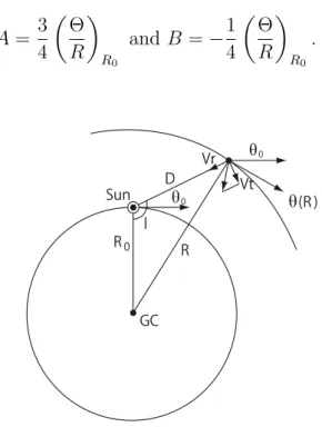
A = 3 4
( Θ R
)
R0
and B = −14( ΘR )
R0
.
Sun
GC R0 R
θ(R ) Vr
D Vt
l
θ0
θ0
Figure 1.11: Geometry of the Sun in the Galactic plane (Sofue 2013). Observed line-of-sight (Vr) and tangential (Vt) velocities can be described using rotation velocity (Θ(R)), galactic longitude (l), and the Galactic constants (Θ0 and R0) (see text).
From equations (1.3) and (1.4), we can easily expect that the line-of-sight and tangential velocities show sinusoidal curves as a function of galactic longitude with a period of 180◦. Oort (1927) confirmedfor the first timethe Galactic rotation using line-of-sight velocity observations, showing the periodic variation (see table 1 in Oort 1927).
Following the Oort’s discovery, a plenty of observations have also confirmed the Galactic rotation (e.g., fig. 1.12). Fig. 1.12 shows the proper motion in Galactic longitude (µlcosb) as a function of Galactic longitude, which display the sinusoidal curve predicted by Oort (1927) (e.g., eq. 1.4). Note that the proper motions were determined by dividing the tangential velocities by the distances from the Sun (e.g., µ = Vt/D =√(µlcosb)2+ (µb)2).
Figure 1.12: The proper motion in Galactic longitude (µlcosb) multiplied by κ, constant value ∼ 4.74 in an unit of km s−1 kpc−1 (Feast & Whitelock 1997). Note that peculiar motions of the Sun (e.g., the standard solar motion) were corrected and the figure was plotted against Galactic longitude (l).
Also, as described in the previous section, radio astronomy has allowed us to observe the entire Galactic disk. Using radio observations, we have seen symmetry of velocity distribution in the Galactic disk just like in the external disk galaxies (e.g., fig. 1.13). Figure 1.13 clearly shows that the Galactic disk is dominated by the Galactic rotation.
100 0 ‒100
‒200 0 200
Galactic longitude (degree)
100 0 ‒100
Galactic longitude (degree) VLSR (km s‒1)
‒200 0 200
VLSR (km s‒1)
Figure 1.13: The position (Galactic longitude l)−velocity (Vlsr) diagram along the Galactic plane (Sofue 2013). (Top) Obtained by HI (21cm) line observation (Nakanishi & Sofue 2003). (Bottom) Obtained by CO(J=1-0) observation (Dame et al. 1987).
1.1.3 Non-circular motions in the disk
The Galactic disk is rotationally supported as described in the previous section (e.g., fig. 1.13), and the circular rotation is known to be an order of ∼ 200 km s−1. Burton (1973) argued that the velocity distribution of the Galactic disk is symmetry relative to the Sun-Galactic center line (but with opposite sign), if the disk is supported by only circular rotation. However, figure 1.14 shows an asym- metric velocity distribution of the Galactic disk obtained from HI observations, which suggests that an additional component, i.e. non-circular motion, also exists in the Galactic disk.
Inner Galaxy
Outer Galaxy
Figure 1.14: Cutoff velocity distribution of the Galactic disk obtained from HI observations (Burton 1973). Horizontal axes show Galactic longitude, and vertical ones represent line-of-sight velocity.
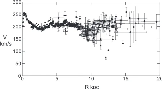
As for asymmetric structures in disk galaxies, spiral arm and bar structures are prominent components. For instance, Sofue et al. (2009) represented Galactic ro- tation velocities as a function of galacto-centric distance (as the Galactic rotation curve) obtained from optical and radio observations. Large errors in outer Galaxy
(R > R0) are due to errors of distance measurements as will be explained in the later section 1.1.4. In fig. 1.15, there are two dip features at R = ∼ 3 kpc and ∼ 9 kpc. The 3-kpc dip may be related to the Galactic bar structure, and the 9-kpc dip may be related to the Galactic spiral structure. Sofue et al. (2009) explained that the 9-kpc dip can be explained, if a ring-like structure with a mass density ratio of
∼ 0.34 relative to the underlying disk density is put at a galacto-centric distance of 11 kpc. In addition, they conclude that the massive ring may be related to the nearby Perseus arm.
Figure 1.15: Rotation velocities as a function of galacto-centric distance (R) (as the Galactic rotation curve) obtained from optical and ra- dio observations (Sofue et al. 2009). The Galactic constants of (R0, Θ0) = (8.0 kpc, 200.0 km s−1) were assumed. For inner Galacxy (R < R0) the tangent velocity method was used, while for outer Galacxy (R > R0) mainly the photometric distance and HIthickness method (Honma & Sofue 1997) were used.
For the dynamics of spiral arms, there have been numerous studies from both theoretical and observational sides. Lin & Shu (1964) proposed the density wave theory (hypothesis) to overcome the winding problem in which spiral structure is destroyed due to the differential rotation (e.g., dΩdR ̸= 0) within several galactic rotations (or several hundreds Myr). In the density-wave hypothesis, asymmetric
(as spiral) potential is assigned in the disk, and it shows rigid rotation (e.g., dΩdRp
= 0) with a pattern speed Ωp, compared to the differential rotation of gas and star with an angular rotation speed Ω(R). This can explain the fact that observed disk galaxies exhibit grand-design spiral arms as quasi-stationary structures in the local universe. The density wave hypothesis can allow us not only to overcome the winding problem, but also to examine a response of gas or stellar motion perturbed by the spiral potential.
Figure 1.16 shows a schematic view of the gas response based on the linear
Figure 1.16: Schematic view of a gas motion perturbed by the spiral potential based on the linear density-wave hypothesis (Burton 1973). Note that Galactic rotation is clockwise.
density-wave hypothesis. One of the important aspects in fig. 1.16 is that non- circular motions (shown as arrows in fig. 1.16) vary periodically between adjacent spiral arms. Following Lin & Shu (1964), Fujimoto (1968) and Roberts (1969) ex-
tended the linear density-wave analysis into the non-linear analysis, in which they found a stationary solution numerically for gas motion perturbed by the density wave. Figures 1.17(a)-(e) show one of the solutions within the co-rotation (CR) ra- dius (e.g., Ω > Ωp), which indicate that shocks occur in front of the spiral potential minimum. The shock is called as the Galactic shock, which enables us to explain systematic non-circular motions with an amplitude of ∼ 20 km s−1 in disk galaxies. Note that in outer co-rotation radius (Ω < Ωp) the shock position is shifted into outer side of the potential minimum, and directions of the non-circular motions are opposite with respect to the case within the CR radius (e.g., Mel’nik et al. 1999). A combination of the density-wave hypothesis and the Galactic shock has been used to explain observational results obtained in the Galaxy (e.g., Roberts 1972; Burton 1973; Mel’nik 1999; Russeil 2007; Sofue et al. 2009).
Roberts (1972) examined non-circular motions in the line-of-sight directions for sources in the Perseus arm with a galactic longitude between 100◦ and 200◦, which was based on optical (photometry and spectroscopy) and radio observations. He concluded that systematic non-circular motions with an amplitude of ∼ 20 km s−1 were found in the Perseus arm for the observed range of galactic longitude, and those could be explained by a combination of the density-wave hypothesis and the Galactic shock.
Russeil (2007) showed differences between the rotation curve model of Brand
& Blitz (1993) and her results determined from photometric and spectroscopic observations for Galactic star-forming regions (see fig. 1.18). Interestingly, quasi- linear variation of the differences (as the non-circular motions) along the galacto- centric distance is appeared in fig. 1.18, which indicates that Galactic co-rotation radius (where Ω = Ωp) is located around the position where the non-circular motion completely disappears. Based on the assumption, Russeil (2007) determined a CR radius of 12.7 kpc based on a linear fitting as shown in fig. 1.18.
Contrary to the density-wave hypothesis, there is an another explanation for the Galactic spiral structure and dynamics, which is recurrent and transient spiral mainly proposed by N-body simulations with/without gas disk (e.g., Miller et al. 1970; Hohl 1971; Hockey & Brownrigg 1974; James & Sellwood 1978; Sellwood & Carlberg 1984; Baba et al. 2010; Wada et al. 2011; Fujii et al. 2011; Grand et
al. 2012; Baba et al. 2013). The main difference between the two explanations is whether the spiral structure exhibits the differential rotation in the same manner as gas and star. In the recurrent and transient spiral, gas flows into local potential minima with irregular motions, and converges to form dense gas cloud near the minimum of stellar spiral potential. Due to the differential rotation, the spiral arm is destroyed (by bifurcation and/or merger with other arms) within a time scale of ∼ 100 Myr (e.g., Wada et al. 2011). As a result, the dense gas cloud is decomposed into inter-arm region with non-circular motions.
In the same way, Baba et al. (2009) argued that observed non-circular motions with an amplitude of ∼ 20 km s−1 can be naturally explained by N-body and hydrodynamical simulation, supporting the recurrent and transient spiral. Baba et al. (2013) also showed that characteristic stellar motions around the spiral arm are shown in evolutionary phases of the spiral arm, which are growing and damping phases (fig. 1.19). Interestingly, direction of the non-circular motions at inner side of the spiral arm in the damping phase is consistent with those predicted by the Galactic shock within the CR (see figures 1.17 (c) & (d) and 1.19 (b) ). However, for the outer side of the spiral arm prediction of the density- wave theory within the CR is different from that of the recurrent and transient spiral in the damping phase. To verify the two explanations for the Galactic spiral structure and dynamics, direct comparison between highly accurate three- dimensional observations and the simulations are required.
Ever since the 1960s, the two scenarios, the Galactic shock based on the density- wave hypothesis and the recurrent and transient spiral, have been proposed and suggested by observations and simulations. However, previous observations were mainly based on the line-of-sight (1D) velocities, which were not enough to compare those with simulation results accurately. In this thesis, we have measured three- dimensional positions and motions toward Galactic star-forming regions based on VLBI astrometry, which enable us to conduct direct and accurate comparison be- tween the observations and the previous researches described above. As a summary of this section, we itemize important points to verify the two scenarios with the 3D positions and motions observations as below:
1. Non-circular motion is systematic (in the density-wave theory) or random (e.g., random gas motions reported in Wada et al. 2011).
2. Direction of the non-circular motions is related to a position of the CR radius (in the density-wave theory).
3. Direction of the non-circular motions is related to phases of spiral evolution (e.g., stellar non-circular motions reported in Baba et al. 2013).
3D positions and motions observations in gas and stellar disks are required to choose the best model, and a large number of those observations with wide cover- age in a spiral arm are also essential.
(a)
(b)
(c)
(d)
(e)
Figure 1.17: Non-linear density-wave analysis for gas motion (Roberts 1969). Stationary solutions were presented at a galacto-centric distance of 10 kpc with a gas dispersion speed of 10 km s−1in specified density- wave parameters, which are a pattern speed (Ωp) of 12.5 km s−1 kpc−1, a pitch angle (i) of ∼ 8◦, and a spiral amplitude (F ) of 5% relative to an axisymmetric gravitational field. (a) Coordinates system in which ξ is parallel to the spiral arm and η is perpendicular to the spiral arm. i is the pitch angle of the spiral arm, and Galactic rotation is counter-clockwise. (b) Relative gas density (σ’ = σ0σ+σ0 1) variation along circular orbit at R = 10 kpc. Subscripts 0 and 1 represent axisymmetric and asymmetric components, respectively. Gas flow is left to right. (c) Velocity variation in the direction of η (e.g., W⊥ = w⊥0 + w⊥1). (d) Velocity variation in the direction of ξ (e.g., W∥ = w∥0 + w∥1). (e) Spiral potential variation.
Figure 1.18: Non-circular motions in the direction of Galactic rotation as a function of galacto-centric distance (Russeil 2007). Circle shows sources in the Perseus arm, and square represents those in the Outer arm.
Growing phase
Damping phase
(a)
(b)
Figure 1.19: Non-circular motions in growing and damping phases of the recurrent and transient spiral revealed by N-body simula- tion (Baba et al. 2013). ξ and η were coordinates assigned in parallel and perpendicular to the spiral arm, respectively. Galactic rotation is aligned with the direction of ϕ. (a) Non-circular motions in the growing phase. (b) Same as (a), but in the damping phase.
1.1.4 Kinematic distance
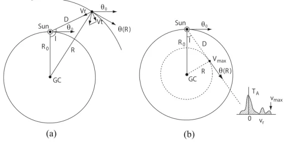
In this section we introduce the most common method to measure a distance in the Milky Way Galaxy, which is the kinematic distance (Dkin). If we cannot measure a distance from the Sun (D) directly, we have to make an assumption to measure a distance. For instance, Merrifield (1992) and Honma & Sofue (1997) assumed that HI-disk thickness of the Galactic disk is the same at any points along a ring with a constant radius to measure a distance (D) using observed apparent thickness. On the other hand, a distance from the Galactic center (R) can be determined based on the assumption of circular motions using the line-of-sight or tangential velocities as shown in equations 1.1 and 1.2. If R is determined with the assumption, immediately the kinematic distance (Dkin) can be described using the law of cosines (e.g., fig. 1.20a) as below:
Dkin =
R0cosl ±
√R2− R0sin2l (inner Galaxy : R ≤ R0) R0cosl +√R2− R0sin2l (outer Galaxy : R > R0).
(1.5)
Clearly, there are two solutions in the case of the inner Galaxy in eq. 1.6. This distance ambiguity is sometimes called as the near-far problem, and therefore one has to use another information such as an absorption feature to discriminate the solutions (e.g., Georgelin & Georgelin 1976). In the outer Galaxy, there is only one solution for the kinematic distance. Another important point is the tangent point where the observed line-of-sight velocity is maximized along the line-of-sight toward the inner Galaxy (see fig. 1.20b). At the tangent point, a distance from the G.C. (R) is written as
R = R0sinl, (1.6)
and therefore the distance to the source (D) is immediately determined as D = R0cosl (see eq. 1.5 or fig. 1.20b). The tangent velocity can be a good tool for determining accurate distances to the Galactic objects located in the tangent points, provided that the Galactic rotation is well-determined by circular rotation. Note that the tangent velocity cannot be observed in the outer Galaxy.
As for the error of the kinematic distance, it depends on amount of non-circular motion of the source as well as location of the source (e.g., Galactic longitude of the
Sun
GC
TA
0 v
r
vmax R
R0
Vmax l
θ0
θ(R ) D Sun
GC R0 R
θ(R ) Vr
D Vt
l
θ0
θ0
(a) (b)
Figure 1.20: Geometry of the Sun in the Galactic plane (Sofue 2013). (a) Kinematic distance (D = Dkin) is determined using line-of-sight velocity (Vr) or tangential velocity (Vt), rotation velocity (Θ(R)), and the Galactic constants (Θ0 and R0) at any point. (b) Ob- servation especially for the tangent point where R = R0 sinl (see text).
source). Sofue (2011) derived an equation for the error of the kinematic distance as below:
δDkin ∼
∂Dkin
∂Vr
δVr = R
3
R0
1
√sin2l(R2− R20sin2l) δVr
Θ(R). (1.7)
Note that Sofue (2011) assumed that the rotation curve (Θ(R)) is a slowly-varying function of Dkin and R so that the rotation curve is recognized as a constant for deriving eq. 1.7. Therefore, eq. 1.7 may not be valid around the G.C. (e.g., R <
∼ 0.5 kpc).
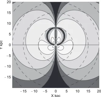
Figure 1.21 represents distribution of errors of the kinematic distance in the Galactic plane derived from eq. 1.7 with an assumed radial velocity error of δVr
= 1 km s−1. Based on eq 1.7 and fig. 1.21, the kinematic distance diverges at Galactic longitude = 0◦ and 180◦. Although the kinematic distance also diverges at the tangent point (where R = R0sinl) based on eq. 1.7, practically the kine- matic distance at the tangent point can be determined well as explained in fig. 1.20b.
Figure 1.21: Accuracy diagram of the kinematic distance in the Galactic plane for δVr = 1 km s−1 (Sofue 2011). Error contours are δDkin= 0.01, 0.02, 0.04, 0.08, 0.16, 0.32, 0.64, ... kpc from white to black. Therefore, around Galactic longitudes of 0◦ and 180◦ direct distance mea- surements such as parallax measurements are essential to determine distances (D) precisely. In this thesis, we present results of VLBI astrometry observations for three star-forming regions, of which one is located at a Galactic longitude of ∼ 171◦. In fact, we will show a significant difference between the kinematic and par- allactic distances for the source in chapter 2. To understand the Galactic spiral structure where peculiar motion (as non-circular motion) could be relatively large, direct distance measurement such as astrometry is crucial.
1.2 VLBI Astrometry
Here we give a brief summary of the principle and position accuracy of VLBI (Very Long Baseline Interferometry) astrometry mainly based on Reid & Honma (2014) and Kameno (2008).
1.2.1 The principle of VLBI
Important observables obtained by VLBI are shown in fig. 1.22 (Kameno 2008). Note that here we consider two-antenna interferometer shown in fig. 1.22 for simplicity, but the concept described here can be also applied to larger array consisting of three or more antennas. Firstly, an emission from the radio source is received at two discrete antennas (e.g., V1(t) and V2(t) in fig. 1.22) with a time lag, τg (i.e., V1(t − τg) = V2(t)). The subscripts 1 and 2 denote antenna 1 and 2, respectively. The lag is called as “geometric delay”, and it is described using the baseline vector ⃗D, source direction vector ⃗s, and the speed of light c as
τg = ⃗s · ⃗D
c . (1.8)
Note that the source direction vector is a unit vector.
Secondly, each signal is recorded at each antenna site with a time tag generated by a clock tied to a frequency standard (e.g., usually a hydrogen maser atomic oscillator). Thirdly, a correction delay, τi, is inserted into antenna 1 (e.g., τ1(t−τi)) to correct the geometric delay relative to the expected source direction which is referred to as the phase-tracking center. In the correlation process, product of the both signals (V1 · V2) with the delay correction is calculated to determine a cross-correlation function C(τ ), which is a function of delay τ as
C(τ ) = lim
T→∞
1 T
∫ t = T2 t = −T2
V1(t − τi)V2∗(t − τ)dt, (1.9) where T is the integration time.
Fourthly, the cross-correlation function is converted into the cross-power spec-
trum ˆC(ν) through the Fourier transform over the lag τ as shown in fig. 1.22. Clearly, the cross-power spectrum is a complex quantity, which is identical to the visibility Vν(u, v) consisting of amplitude and phase information. Here u and v are called as the spatial frequency, which are defined as u = Dλx and v = Dλy. Here Dx
or Dy is the baseline vector in the east-west or north-south direction, respectively, and λ is the observing wavelength.
Figure 1.22: Important observables obtained by VLBI (Kameno 2008). Image was adapted from Kameno (2008) at http://milkyway.sci.kagoshima-u.ac.jp/˜kameno/SS2008/.
Finally, the visibility with the (u, v)-domain can be converted into the intensity distribution Iν(l, m) on the sky with the (l, m)-domain through the inverse Fourier
transform. This relation is known as the Van Cittert-Zernike Theorem. l and m denote angular offsets relative to the phase-tracking center in the east-west and north-south directions on the sky, respectively (see fig. 1.22).
1.2.2 Position Accuracy of Absolute Astrometry
As for the position accuracy (∆s) of VLBI astrometry, it can be roughly estimated by using eq. 1.8 as
∆s ≈ c∆τDg, (1.10)
where ∆τg is an uncertainty of the geometric delay measurement. Clearly, one can easily expect that longer baseline provides better position accuracy, and therefore VLBI technique has been used to conduct an accurate astrometry with baseline lengths larger than 2,000 km (e.g., VERA; VLBA). Moreover, eq. 1.10 shows that reducing the delay uncertainty allows us to obtain a better position accuracy. The delay uncertainty can be decomposed into
∆τg = ∆τtropo+ ∆τiono+ ∆τstat+ ∆τinst+ ∆τstruc+ ∆τtherm. (1.11) Here ∆τtropoand ∆τionoare errors of tropospheric and ionospheric delays, which are related to atmospheric condition. ∆τstat is the station delay error (e.g., occurred due to station position error). ∆τinstis the instrumental delay error (e.g., occurred due to signal propagation in antenna and cables). ∆τstruc is caused by the source structure, and ∆τtherm is the thermal delay error (e.g., random error depending on SNR).
It has been known that ∆τtropo is the dominant term (typically ∼2 cm in delay length converted by c∆τtropo) in VLBI astrometry with observing frequencies larger than 10 GHz (e.g., Reid & Honma 2014). Note that below 10 GHz frequencies one also has to concern about ∆τiono, since the term is proportional to λ2. If one assumes c∆τg = 2 cm and D = 8,000 km in eq. 1.10, then the resultant position accuracy is ∼0.5 mas. The assumed baseline length has been achieved in current VLBI array (e.g., VLBA). In fact, the resultant position accuracy is basically consistent with position accuracies of the ICRF (International Celestial
Reference Frame) radio sources (mainly QSOs) determined by broad-band VLBI observations.
Therefore, ∼0.5 mas is a typical position accuracy of absolute VLBI astrometry. However, it is not enough to conduct kpc-scales astrometry, and for this reason relative astrometry should be required.
1.2.3 Position Accuracy of Relative Astrometry
Relative astrometry referred to “phase-referencing” is the key to reduce the atmospheric phase fluctuation, and the method can achieve better accuracy in VLBI astrometry. In the relative astrometry, visibility phase of a reference (e.g., QSO) is subtracted from that of a target. The phase difference tells us an angular position offsets of the target source relative to the reference source. If one chooses a distant QSO as a reference source (e.g., QSO with negligible parallax and proper motion), then one can measure an absolute parallax and proper motion of the target source just like the absolute astrometry in the relative astrometry.
For a position accuracy of the relative astrometry, we can evaluate this using the delay difference,
∆(s1− s2) ≈
c∆(τg,1− τg,2)
D (1.12)
where
∆(τg,1− τg,2) =∆(τtropo,1− τtropo,2) + ∆(τiono,1− τiono,2) + ∆(τstat,1− τstat,2)
∆(τinst,1− τinst,2) + ∆(τstruc,1− τstruc,2) + ∆(τtherm,1− τtherm,2(1.13)). Here subscripts 1 and 2 define target and reference sources instead of antennas 1 and 2 used previously. τstruc is referred to the “baseline-based quantity”, while the other terms except for the τtherm are referred to the “station-based quantity”. τstruc is 0 if the source has point-like structure, and therefore point-like QSOs can be good reference sources. Even though a source has diffuse structure like jet, the term can be corrected in data analysis with the self-calibration method (e.g., Reid
& Honma 2014). The station-based quantity depends on each antenna, meaning that the terms can be cancelled out effectively using the relative astrometry with
an adjacent reference source. Note that for VERA array an additional correction for τinst has been conducted, since independent two receivers are installed in each VERA antenna for the 2-beam observation (e.g., τinst,1 − τinst,2 ̸= 0 in the VERA array). Detail of the 2-beam calibration is summarized in Honma et al. (2008a).
As described previously, the dominant error term is ∆τtropo for the absolute astrometry with observing frequencies larger than 10 GHz. In the same way, the dominant error term in the relative astrometry is c∆(τtropo,1− τtropo,2), and it can be described as
∆(τtropo,1− τtropo,2) = cτ0(secZ1 − secZ2) ≈ cτ0 secZ tanZ ∆Z, (1.14) where Z is a zenith angle with ∆Z = (Z1 − Z2), Z is an averaged zenith angle, and τ0 is a tropospheric zenith delay residual (e.g., typically ∼2 cm in delay length converted by cτ0 as described previously). As an order estimation, we may roughly regard ∆Z as a separation angle (θsep) between the source and reference sources, and thus eq. 1.12 could be modified using eq. 1.14 as
c∆(τg,1− τg,2)
D ≈
cτ0
D θsep at Z = 40
◦. (1.15)
Clearly, the reduction factor, θsep, is multiplied in eq. 1.15 for the relative astrom- etry compared to eq. 1.10 for the absolute astrometry. This is the main difference between the two methods. Again, if one assumes c∆τg = 2 cm and D = 8,000 km, but with θsep = 1 deg in eq. 1.15, a position accuracy in the relative astrometry is
∼ 10 micro-arcsecond (µas) compared to ∼ 0.5 mas (∼ 500 µas) in the absolute astrometry!
Strictly speaking, it is difficult to estimate a position accuracy of VLBI astrome- try with a precise analytical expression, and thus simulations have been conducted for the estimation (e.g., Pradel, Charlot, & Lestrade 2006; Honma, Tamura, & Reid 2008). Pradel, Charlot, & Lestrade (2006) showed that the tropospheric de- lay residual can be the dominant error source in VLBI astrometry. According to Honma, Tamura, & Reid (2008b), position accuracies of the relative astrometry in east-west and north-south directions are related to source’s parameters as declina- tion (δ), zenith delay error, the separation angle, and position angle of the target
source relative to the reference source (see figures 5-7 in Honma, Tamura, & Reid 2008b). We itemize important points to obtain a better position accuracy in the VERA astrometry based on Honma, Tamura, & Reid (2008b),
1. High declination (e.g., δ > 15◦).
2. Small separation angle (e.g., less than 1◦).
As a summary of this section, the relative astrometry has a potential to conduct kpc-scales astrometry for understanding Galactic spiral structure and it’s three-dimensional motion. Toward the goal, we will report three results of VERA astrometry related to the Perseus arm in this thesis.
1.2.4 Sensitivity
VLBI (relative) astrometry allows us to conduct Galactic scale astrometry with a position accuracy of ∼10 µas level as described in previous section. However, in VLBI, observed source size (Θ0) should be comparable to or smaller than an angular resolution of VLBI, Dλ, otherwise source flux is reduced significantly with source size larger than the angular resolution of VLBI (e.g., Sasao & Fletcher 2005). This condition for VLBI is described as
Θ0 ≤ λ
D, (1.16)
where λ is the wavelength and D is the baseline length in VLBI observation. Using Eq. (1.16), we can write the intensity Iν and flux density Fν of the source as below:
Iν = 2kTB λ2 ≤
2kTB
Θ20D2, and Fν = 2kTB
λ2 πΘ20
4 ≤
πkTB
2D2 , (1.17) where k = 1.381 × 10⁻²³J・K−1is the Boltzmann constant and TBis the brightness temperature of the source. If we set the minimum detectable flux density (Sνmin) by VLBI, we can write the lower limit (TBmin) to the brightness temperature for
the detectable source using eq. 1.17 as
TBmin ≃
2D2
πk Fνmin. (1.18)
If we set D = 2,300 km and Sνmin = 0.16 Jy referred from the VERA Status Report1 in Eq. (1.18), then TBmin ≃ 4×10⁸ K. This means that VLBI astrometry can observe only compact and non-thermal sources such as AGNs, masers, and pulsars but thermal sources such as stars and molecular clouds.
In this thesis, we especially focus on the masers to conduct Galactic scale astrometry because a large number of masers are distributed in the Galactic star- forming regions, and also they are bright and compact enough for VLBI astrometry as explained in next section.
1.2.5 Target: 22 GHz H
2O maser
Maser (Microwave Amplification by Stimulated Emission of Radiation) is analo- gous to laser (Light Amplification by Stimulated Emission of Radiation) occurred at optical band, but maser is occurred at radio band. In thermal equilibrium, number density distribution of particles obeys the Boltzmann distribution:
n2/g2
n1/g1 = exp(−
hν
kT) < 1. (1.19)
Here n1 and n2 are the number densities in the energy states 1 and 2, and g1 and g2 are the statistical weights in the each energy state. Note that the energy state 2 is higher than the energy state 1. h and ν are the Planck constant and frequency, while k and T are the Boltzmann constant and temperature of material composed of the particles. In contrast to the Boltzmann distribution, maser occurs when the population is inverted (e.g., ng1
1 <
n2
g2). In such a special condition (as the inverted condition), the absorption coefficient (αν) can be negative as shown in
1http://veraserver.mtk.nao.ac.jp/restricted/CFP2012/status12.pdf
below equation (Rybicki & Lightman 1979):
αν = hν
4πn1B12(1 − n2/g2
n1/g1
)ϕ(ν). (1.20)
Here B12 is the Einstein B-coefficient related with probability of energy transition by absorption, and ϕ(ν) is the line profile function that describes absorption effec- tiveness in each frequency.
Considering the radiative transfer equation with the negative absorption coef- ficient, we can expect an occurrence of significant amplification as shown below:
Iν(τν) = Sν + e−τν(Iν(s0) − Sν), (1.21) where Sν ≡
jν
αν
< 0 and τν =
∫ s s0
αν(s′)ds′ < 0.
Here Sν and τν are the source function and optical depth, while Iν(s0) and jν are the incident radiation and emission coefficient. The equation shows that the inci- dent radiation is amplified exponentially with the negative absorption coefficient. If we assume τν = −100 in the inverted population, then the incident radiation is amplified by a factor of 1043, leading to significantly large brightness temperature. Therefore, maser can be a good probe for the VLBI astrometry as explained in previous section.
As for history of the astronomical masers, 18 cm OH maser, the first astro- nomical maser, was observed and discovered by Weaver et al. (1965, Nature) in Galactic star-forming regions. After the discovery, H2O masers at 22 GHz were also observed by Cheung et al. (1969, Nature) in Galactic star-forming regions. Other interstellar molecules have also displayed maser emissions in star-forming regions and/or around late-type stars (e.g., SiO, CH, HCN, CH3OH, H2CO and NH3). H2O masers in star-forming regions are thought to be excited by outflows emitted from embedded young stellar objects (YSOs) as suggested by Strelnit- skij & Sunayev (1973), who showed the association between H2O maser and high velocity flows. We list properties of H2O maser in table 1.1, and also represent known energy transitions for H2O masers including the 22 GHz emission in fig. 1.23 (Gray, 2012). Table 1.1 shows that H2O maser is formed in a dense and high
Table 1.1: H2O Maser Line in Star-Foring Regions (Stahler & Palla 2005)∗ Molecule Transition Type Frequency Eupp/kB n T
(GHz) (K) (cm−3) (K)
H2O JK−1K=616→ 523 rotational 22.2 640 107−109 300-1000
∗ E
uppis the energy of the upper state above ground. n and T are density and temperature over which emission occurs.
temperature region as a molecular core embedded in a star-forming region. The size of H2O maser is known to be a few AUs (astronomical units) as shown in fig. 1.24 (Genzel et al. 1981). Almost all masers in fig. 1.24 show angular sizes of ≤ 0.1−0.3 milli-arcsecond (mas), corresponding to linear diameters of ≤ 0.8−2.3 × 1013 cm (≤ 0.5−1.5 AU) at the distance of W51M, which is 5.41 kpc (Sato et al. 2010b).
Finally, we itemize important H2O maser properties as below:
1. The emission is significantly bright (TB ∼ 1012 K from fig. 1.24) in contrast to thermal emissions.
2. Maser has compact and point-like structures.
3. The emission shows linear polarization (e.g., Bologna et al. 1975).
4. Line width of the emission is narrow since velocity coherence is necessary for the emission (e.g., Gray 2012).
Based on the above properties, H2O maser can be a good probe to conduct VLBI astrometry, and therefore we have observed H2O masers associated with Galactic star-forming regions in this thesis.
Figure 1.23: A subset of the energy lebels of H2O showing the known maser transitions (Gray, 2012).
Figure 1.24: Distribution of maser spot sizes in W51M (Genzel et al. 1981). (Top) Flux density vs the spot size. Spots lower than 1 milli- arcsecond (mas) are unresolved (vertical dotted line), and there- fore only upper limits are shown for the spots (arrows). Solid lines represent constant brightness temperatures (K). (Bottom) Number count vs spot size. Spot sizes were determined by de- convolution in the direction of right ascension (R.A.). Note that spots lower than 1 mas only show upper limits.