A Highly Efficient Consolidated Platform
for Stream Computing and Hadoop
Hiroya Matsuura
Tokyo Institute of Technology 2-12-2 Oookayama, Meguro-ku,
Tokyo, Japan, 152-8550
[email protected]
Masaru Ganse
Tokyo Institute of Technology 2-12-2 Oookayama, Meguro-ku,
Tokyo, Japan, 152-8550
[email protected]
Toyotaro Suzumura
Tokyo Insitute of Technology / IBM Research Tokyo 1623-14 Shimotsuruma, Yamato-shi,
Kanagawa-ken, Japan, 242-8502
[email protected]
ABSTRACT
Data Stream Processing or stream computing is the new computing paradigm for processing a massive amount of streaming data in real-time without storing them in secondary storage. In this paper we propose an integrated execution platform for Data Stream Processing and Hadoop with dynamic load balancing mechanism to realize an efficient operation of computer systems and reduction of latency of Data Stream Processing. Our implementation is built on top of System S, a distributed data stream processing system developed by IBM Research. Our experimental results show that our load balancing mechanism could increase CPU usage from 47.77% to 72.14% when compared to the one with no load balancing. Moreover, the result shows that latency for stream processing jobs are kept low even in a bursty situation by dynamically allocating more compute resources to stream processing jobs.
Categories and Subject Descriptors
D.3.3 [Resource management, scheduling, and load- balancing]: Language Contracts and Features – abstract data types, polymorphism, control structures. This is just an example, please use the correct category and subject descriptors for your submission. The ACM Computing Classification Scheme: http://www.acm.org/class/1998/
Keywords
DSMS, Data Stream Processing, MapReduce, Hadoop, Dynamic Load Balancing.
1. Introduction
Data Stream Processing [1][2][3][4][5][6][7] is the notion of processing incoming data from various data sources such as sensor, web click data, IP log, etc. on memory to realize real-time computation. This computing paradigm is getting important since business organizations need to react any event relevant to their revenue. On the other hand, batch processing (which has been around for a long time) is also an essential computing paradigm since data stream computing can only access data that resides in memory. Lots of applications need to access entire data to perform macro analysis.
Meanwhile, data stream processing has become a hot research area since early 2000s with projects such as Borealis [1] and TelegraphCQ [2]. As of today, lots of commercial softwares are appearing such as IBM System S [4][5][6][7]. However, traditional batch computing still has a critical role in the era of data explosion. Such a representative system is Hadoop [8], an open source software originally developed by Yahoo. Hadoop is a
distributed data processing platform which allows users to easily create parallel and distributed applications in what they call MapReduce [9] programming model.
Both the above mentioned computing paradigms are highly important and there are strong demands in business areas for them. Therefore systems based on the two computing paradigms are simultaneously executed using same computing resources rather than running them in different resource environments.
This demand strongly comes from the need of optimizing and reducing power consumption by fully utilizing computing resources and making the CPU usage close to 100% as much as possible, which leads to maximum efficient use of computing resources.
Meanwhile, data stream processing considers that the resource time or latency to obtain final results are bound by SLA (Service Level Agreement) given by each application. Ultimate examples include algorithm trading in financial institutions which requires resource times in the order of microseconds. This latency requirement varies in different business domains, so there are some business areas that only expect the latency in the order of seconds. Moreover the concept of traditional batch computing such as Hadoop only emphasizes high throughput, and does not consider the latency strictly although some batch processing computes on a dead-line basis.
In this research we propose an integrated execution platform that efficiently executes both data stream processing and traditional batch processing such as Hadoop while satisfying the requirement of SLA given by the data stream processing applications and increasing the maximum use of given limited computing resources. The assumption in this research is that additional computing power can not be added based on the real business case. This limitation is realistic due to various reasons such as space, budget, and electricity limitations. Our contributions in this paper are as follows:
(1) We built an integrated execution platform that effectively switches both data stream processing and batch processing based on incoming traffic to maximize the use of finite computing resources. Our proposed system improves effective use of CPU by 23.47 % when compared to no effective scheduling policy while keeping the SLA given by data stream processing application requirements.
(2) To realize the efficient dynamic load balancing algorithm, we adopt a time series prediction algorithm with low computational complexity, and we show that this prediction algorithm hits around 98% accuracy using real data.
2012 IEEE 26th International Parallel and Distributed Processing Symposium Workshops 2012 IEEE 26th International Parallel and Distributed Processing Symposium Workshops & PhD Forum
(3) To build an integrated execution platform, we use Hadoop as a representative batch processing system and extend the system so as to dynamically adjust the number of physical nodes that Hadoop daemon runs. We also prepared the interface that allows other external software components to control such dynamical adjustment of running nodes.
This paper is organized as follows. We explain the Integrated Execution Platform (IEP) in Section 2. Section 3 presents construction and implementation of IEP. We describe the time series prediction algorithm that estimates future changes of work loads under Section 4. Evaluation of our approach is provided in Section 5.3 Contributions of this paper in the context of related work is described in Section 6. Conclusion of this paper is presented in Section 7.
2. Integrated Execution Platform for Data
Stream Processing and Batch Processing
In this section we describe the motivation on why we need a consolidated platform of two computing paradigms, data stream processing and batch processing, and then motivating examples.
2.1 Motivation
Although data stream processing is a key factor for enabling real-time computation for vast amount of incoming data from various sources, batch processing (store-and-process model) is still necessary computing paradigm in the situation that data analysis is only meaningful by processing all the data.
For example, in telecommunication industry, real-time fraud detection is performed by data stream processing, whereas the whole social network analysis for all the CDR(Call Detail Record) is realized by traditional batch processing.
In real business environment, many business parties only have some amount of limited computing resources and it is difficult to invest in additional computing facilities because of various reasons such as financial cost, electricity, space limitation and so forth. Therefore, even though business users consider new computational applications are required such as data stream processing applications, the issues mentioned above would remain as high obstacles.
Given such real business scenarios and needs, we propose an integrated platform for two important computing paradigms, data stream processing and batch processing. The strong assumption in our proposed research is that the amount of computational capacity is strictly limited and new capacity can not be added due to the above reasons.
The reasons for why such an integrated execution platform is meaningful are as follows. First, the amount of incoming data for data stream processing is often stable and is unpredictable. E.g. In the case of Twitter stream monitoring, there could be a burst situation in case that some sudden incident happens. Some data stream applications can have periodic traffic patterns. E.g. Again in the case of Twitter streams, although traffic is low at daytime, it becomes very high at night.
The basic assumption of data stream processing is that latency is critical as compared to batch processing. But batch processing is looser and the latency is not really critical even though some applications have deadlines to finish the computation. Especially batch processing is typically executed at night or on holidays after all the data to be processed were accumulated.
We argue that such different characteristics of data stream processing and batch processing should be leveraged and we can design and implement an integrated execution platform by using those different characteristics. Computational efficiency would be highly improved by the proposed system since either computational paradigm will be executed depending on the traffic pattern and the SLAs (Service Level Agreement) provided by two paradigms. Moreover from the perspective of electricity consump- tion, improved computational efficiency will be important factor considering the fact that the electricity consumption is not different at busy time when compared to idle time.
2.2 Effective Application Scenarios
There exist many effective application scenarios in various domains. The example scenarios are as follows:
(1) Internet Shopping Site
For data stream processing, web server log monitoring is important to detect distributed DoS (Denial-of-Service) attacks. Other applications include click stream to understand customers' behavior in real-time, word pattern matching for Twitter stream data.
On the other hand, some example applications for batch processing include generation of inverted index for web search, and compute collaborative filtering for the purpose of marketing. (2) Financial Trading Institution
For data stream processing, an automatic algorithm trading is becoming common in many financial trading institutions and realizing very low latency for such an application is greatly critical to win over other institutions. On the other hand, more long-running trend analysis is an important example of batch processing.
(3) Telecommunications Industry
Current smart phones are equipped with many sensor devices such as communication device, GPS, electrical money, etc. Many telecommunication companies are keen on those data to detect subscriber's behavior to learn new business opportunities or sell those data to other various industries since the sensor data includes many important information on subscriber's behavior.
2.3 Goal : Maximizing Resource Utilization
The important point in this research is to pursuit how resource utilization is maximized. That means that we do not necessarily make the latency as low as possible in the data stream processing applications, and it is important to keep the latency close to the threshold without avoiding the latency divergence. This leads to high resource utilization. This is our target goal of our research.
3. System S and Hadoop
In this section, we provide the overview of two representative systems, System S as a data stream processing platform and Hadoop as a batch processing platform.
3.1 System S: Data Stream Processing Platform
System S [4][5][6][7] is large-scale, distributed data stream processing middleware under development at IBM Research. It processes structured and unstructured data streams and can be scaled to a large numbers of compute nodes. The System S runtime can execute a large number of long-running jobs (queries) in the form of data-flow graphs described in its special stream-
application language called SPADE (Stream Processing Application Declarative Engine) [5]. SPADE is a stream-centric and operator-based language for stream processing applications for System S, and also supports all of the basic stream-relational operators with rich windowing semantics. Here are the main built- in operators mentioned in this paper:
Functor: adds attributes, removes attributes, filters tuples, maps output attributes to a function of input attributes
Aggregate: window-based aggregates, with groupings Join: window-based binary stream join
Sort: window-based approximate sorting Barrier: synchronizes multiple streams
Split: splits the incoming tuples for different operators
Source: ingests data from outside sources such as network sockets Sink: publishes data to outside destinations such as network
sockets, databases, or file systems
SPADE also allows users to create customized operations with analytic code or legacy code written in C/C++ or Java. Such an operator is a UDOP (User- Defined Operator), and it has a critical role in providing flexibility for System S. Developers can use built-in operators and UDOPs to build data-flow graphs. After a developer writes a SPADE program, the SPADE compiler creates executables, shell scripts, other configurations, and then assembles the executable files. The compiler optimizes the code with statically available information such as the current status of the CPU utilization or other profiled information. System S also has a runtime optimization system, SODA [7]. For additional details on these techniques, please refer to [4][5][6][7]. SPADE uses code generation to fuse operators with PEs. The PE code generator produces code that (1) fetches tuples from the PE input buffers and relays them to the operators within, (2) receives tuples from operators within and inserts them into the PE output buffers, and (3) for all of the intra-PE connections between the operators, it fuses the outputs of operators with the downstream inputs using function calls. In other words, when going from a SPADE program to the actual deployable distributed program, the logical streams may be implemented as simple function calls (for fused operators) for pointer exchanges (across PEs in the same computational node) to network communications (for PEs sitting on different computational nodes). This code generation approach is extremely powerful because simple recompilation can go from a fully fused application to a fully distributed version, adapting to different ratios of processing to I/O provided by different comput- ational architectures (such as blade centers versus Blue Gene).
3.2 MapReduce and Apache Hadoop
MapReduce [9] is a programming paradigm proposed by Google. With this concept, we can deal with peta-byte scale data on thousands of computers. The concept of MapReduce programming model is based on map and reduce notion in the functional languages. With this programming model, we can enjoy parallelism by implementing two methods, map and reduce. MapReduce engine automatically distributes the data, processes them by Map function and integrates them by Reduce function. We need not to consider the processing daemons, fault tolerance and communications.
Hadoop [8] is one of the implementation of MapReduce programming model implemented by Yahoo. In our paper, this computing paradigm is referred as “batch processing” since the
entire data is stored in disks rather than processing them on memory.
4. Integrated Execution Platform
In this section we describe the overall design and implementation of the proposed integrated execution platform.
4.1 System Overview
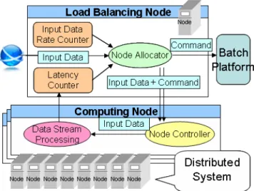
An Integrated Execution Platform (we refer IEP hereafter) is comprised of three software components, a data stream processing platform and a batch processing platform, and then dynamic load balancing component. Figure 1 illustrates the overall architecture of the Integrated Execution Platform that runs on top of a shared cluster of multiple compute nodes. One representative node in a cluster that runs dynamic load balancing component is responsible for allocating nodes to either two platforms based on our proposed scheduling strategy. A dynamic load balancing component observes the input data rate and latency, and determines the node assignment strategy for each task. It uses the predicted input data rate by time series prediction algorithm. The detail strategy and algorithm is described in Section 5.
Batch processing platform with dynamic node assignment system is the second component. It must run manifold batch processing applications on distributed systems and switch calculation node assignment. Node switching speed and cost are related with task granularity. Less task granularity results in less node switching cost.
Data Stream Management System (DSMS) [1][2][3][4][5][6][7] with dynamic node assignment is the third. It must run multiple applications in distributed environment. Many DSMS are supplied as middleware systems to facilitate this demand.
We can construct IEP by combining the components to satisfy above requirements.
4.2 Implementation on System S
Dynamic Load Balancing unit and time series prediction algorithm are implemented on System S because of its flexibility. Fig.1 shows the dynamic load balancing unit and Data Stream Processing unit. Many modules of this system are written in built- in operators of SPADE. The three modules required for our integrated execution platform, a word matching program (one of
Figure 1 Architecture of Integrated Execution Platform
applications), node assignment module, time series prediction program are all written in C++ as SPADE user defined operators. We have implemented a text matching program as a UDOP that takes arbitrary keywords to be monitored as input.
4.3 Extending Hadoop
In order to suspend or resume the job controlled by Hadoop, we extended Hadoop to support such a suspend/resume mechanism and implemented the external interface that allows external software components to invoke the extended mechanism of Hadoop. Hadoop is designed to have a fail-over or fault-tolerance feature in the case of any failures at compute nodes, but it takes more than a couple of minutes to detect such a failure. However dynamic load balancing of the Integrated Execution Platform described in this paper need to detect such a failure in the order of seconds to change the node assignment. Therefore we cannot use the existing fail-over feature of Hadoop. Furthermore the current Hadoop implementation does not have a mechanism to dynamically assign new compute nodes at runtime. Those are the reasons for why we extended Hadoop.
To extend Hadoop to facilitate the above mentioned suspend/resume mechanism, we modified the central daemon called “JobTracker” that is responsible for distributing multiple tasks to multiple compute nodes. Each map and reduce processing in Hadoop is called a “task” and a bag of tasks for each application is called a “job”. A job is submitted to a JobTracker after storing all the required data on the distributed file system called HDFS (Hadoop Distributed File System) [8]. Then the JobTracker accepts the submitted job and maintains it by dividing a job into a set of tasks internally. Meanwhile, there is a daemon called “TaskTracker” at each compute node that sends a heart beat message to the JobTracker. The heart beat message is also used for fault-tolerance but it also contains CPU usage and the status of each task, and then those information is used for the task scheduling in the JobTracker daemon. Once a JobTracker receives a heart beat message from each TaskTracker, the JobTracker responses to the TaskTracker with new task when the JobTracker decides that the TaskTracker is ready for handling new task.
We also extended the JobTracker daemon to have a status repository for TaskTrackers that maintains which TaskTracker is currently suspended or ready. By looking at the information, the JobTracker can understand whether it can assign new tasks or not. Furthermore we modified the JobTracker daemon to allow external programs or components such as Data Stream Processing Systems (e.g. System S) to control the above mentioned TaskTracker status repository. The status repository is refreshed by receiving a command from a TCP socket port. The command includes which TaskTracker should be suspended or resumed. By making such a control facility in the JobTracker daemon, we can fulfill the above functional requirement that needs to modify the
node assignment in near real-time.
In our current extension of Hadoop, suspend / resume per “node” is supported but suspend / resume per “process” has not been supported yet. Therefore if there are running tasks (multiple processes), we have to wait until all the tasks are finished. To avoid this situation, process-based suspend / resume function and the functionality for forcing task termination and re-execution is needed.
4.4 Dynamic Load Balancing
We use two information for node allocation strategy. One information is the predicted input data induced by our time-series prediction algorithm described in the next section, and the other information is the latency obtained by computation at all the compute nodes. Based on one of the above information, the node allocation component decides whether it allocates each node to either data stream processing or batch processing.
As for the scheduling strategy based on the data input rate, our time-series prediction algorithm predicts input data rate, and then the appropriate node number is determined by dividing the predicted input data rate by the input data rate that can be properly handled by one single compute node. Our scheduling strategy allows one to add only single node at once by avoiding the additional cost of switching compute nodes and also considering the over capacity planning possibly caused by the singular value computed by our prediction algorithm. The node assignment is conducted every time the input data rate is refreshed.
Latency for all the computing nodes are measured constantly and changing the node assignment is also done by those measured latency data. However, changing the node assignment based on latency is only performed when the measured latency is over the threshold. In the case that such a situation has occurred multiple times, the node assignment strategy decides to add one additional compute node regardless of input data rate. The system constantly counts the number of such a situation, and we call the count
“violation count”. The violation count is reset when the node assignment is changed.
In our current implementation, we assign the violation count to 40 and the node assignment is changed when the violation count is set to 40. When the violation count is too small and the latency threshold is too low, the number of adding nodes for data stream processing becomes too big and there will be a situation where batching processing is never ended.
Apart from this, we implemented the latency for each compute node. At a head node which dynamic load balancing and Hadoop’s JobTracker is executed, the processing tends to be overloaded and the latency tends to be high when compared to other compute nodes. If our system detects that the latency of the head node is close to the threshold, the system controls a head node to stop processing the incoming data.
With the above three mechanisms and the time-series prediction algorithm described in Section 4, we implemented dynamically load balancing mechanism in our integrated execution platform.
5. Time Series Prediction Algorithm
We employ time series model for our prediction algorithm in order to improve our current dynamic load balancing system. We choose the SDAR (Sequentially Discounting Auto Regression) model, which is a transformation of AR model and used in the
change point detector, ChangeFinder [11], for time series prediction algorithm.
For the change point detection algorithm for time-series data streams, we employed the SDAR (Sequentially Discounting Auto Regressive model estimation) algorithm proposed by Yamanashi et al. [??]. Many efforts [??] [??] have proposed a change point detection algorithm, but most of them assumes that data streams are stationary, does not deal with non-stationary data streams. The AR (Auto-Regressive) model is one of the most typical models to represent a statistical behavior of time series data in statistics. However, most existing algorithms of estimating parameters for the AR model is designed under the assumption that the data source is stationary. Many data streams in the area of stream computing is characterized as non-stationary data streams. In the case of micro blogging examples such as Twitter, the data source become non-stationary when sudden important event is occurred. The SDAR algorithm deals with non-stationary data sources by introducing a discounting parameter to the AR model estimation algorithm so that so that the effect of past examples can gradually be discounted as time goes on.
5.1 Dimensionality of SDAR Model
An important factor to consider when deciding the model is how we determine dimension. To request the best dimension dynamically, it is necessary to discover a locally regular part in non-regular time series and decide the best dimension to the time series of each locally regular part. But the calculation is very complex, so it is very difficult to use it for a dynamic (real-time) load balancing. In short, an algorithm that is appropriate for a dynamic load balancing does not exist now. It would be possible to decide the dimension statically, but a decrease in the predictive performance might be caused because it deals with the time series data that has a change different from usually that is not already known. In addition, SDAR model values the computational complexity decrease more than the pursuit of accuracy, so we decide single dimension for forecast. It is thought that the decrease of accuracy can be supplemented by making the acquisition rate of input data detailed.
5.2 Forecast with SDAR Model
There is a problem in time series model that uses the SDAR model. The algorithm using the SDAR model corresponds to non- regular time series by using the effect of oblivious characteristics. In other words it cannot correspond to non-regular time series until oblivious is done. Therefore, more flexible algorithm to correspond for "Rapid change in the time series" is needed. Because the SDAR algorithm is an algorithm used by “Changing Point Detection Engine Change Finder” (Changing Point is
“rapidly changing point of time series behavior”), correspondence to non-regular time series and forecasting can be done at the same time by using the calculation of ChangeFinder without newly increasing the computational complexity. In this algorithm, when the time series is not rapidly changed, the actual measurement value always takes the value between the predictive value and the threshold except the mere case of an outlier. Because it is imposs- ible to forecast a mere outlier, this can do nothing but be given up. Selection of the predictive value when detecting a changing point remains as a problem to be solved. While currently we forecast with wide threshold, in future it is necessary to make an algorithm that decides the threshold by the size of the changing point.
5.3 Implementation
This algorithm is implemented by using System S and evaluated by using real data. We use SPADE in easy operation, and use a UDOP by using C++ in complex operation. An application implemented by System S can be built into other one just as a module, or be possible to refer from other programs by the Socket communication etc. An application implemented by System S can be built in to another program just as a module or be possibly referred from other programs by socket communication etc. Therefore we can reuse this algorithm in other applications. We use Twitter stream data between 2010/4/1~2010/4/5 as input data by using Streaming API of Twitter. By using Twitter Streaming API, vast amount of tweet data can be obtained in real time even though the whole data can not be retrieved. This experimental data was used for an integrated execution platform. For the Twitter data obtained every one minute, the hitting ratio of our time-series prediction algorithm was 98.0403% when comparing the predicted value and real value. The maximum value of the error margin was 114.8334, the median was 14.7822, and the average was 22.79787. The unit is number of responses, and real data of responses change between 100 to 800.
We use a time series prediction algorithm with relatively low computational complexity. We consider that our algorithm could be enhanced by considering the periodicity of the incoming sensor data. However, our basic assumption for this prediction is that those algorithms should be light computational complexity when applying the algorithm to load balancing.
6. Performance Evaluation
This section describes the validity of our proposed system by assuming the system that conducts real-time keyword monitoring as data stream processing and conducts inverted index construction as batch processing.
6.1 Experimental Scenario and Implementation
Assume that we construct a consolidated system in a shared cluster that conducts both data stream processing and batch processing. As data stream processing, the system receives Twitter streams and finds important Tweets in real time to detect important events such as earthquake and the announcement of new products. On the other hand, as batch processing, the system constructs inverted index of all the received Twitter messages to provide a search interface.
We implemented regular expression-based keyword matching as an UDOP(User-Defined Operator) operator with System S and used the source code published by Yahoo Hadoop Tutorial [10] to compute Inverted Index on Hadoop.
6.2 Experimental Environment
We use 8 compute nodes and 2 administrative nodes connected by 1 Gbps Ethernet. One of the administrative nodes send data to compute nodes, and the other of the nodes stores the information with regards to measured performance information such as latency. One of 8 compute nodes is also responsible for providing the IEP system and Hadoop’s management daemon including JobTracker and NameNode (for Hadoop Distributed File System) daemons. The home directories of these nodes are shared with an NFS server. In order to avoid the inaccurate time measurement by the I/O bottleneck caused by NFS, input data is allocated on a RAM Disk of administrative nodes. The input data is sent over TCP
with a Ruby script. The script controls the data emission rate in order to simulate data rate that contains low, high, and burst data rate as shown in Figure 2. The low data rate is around 200 tuples per second that can be processed by one single node. The high data rate is around 3500 tuples that might cause the latency divergence with 4 nodes. We also articulate the burst rate two times during the experimental period. This three patterns of data rate, low, high and burst will be used in Section 6.6
The experimental environment is as follows. Each compute node has dual Opteron 1.6GHz CPU with 4GB DRAM. The two administrative nodes have dual Opteron 1.6GHz CPU with 8GB DRAM. Software environments are CentOS 5.4 kernel 2.6 for AMD64, InfoSphere Streams 1.2 (System S) as data stream computing platform, Apache Hadoop 0.20.2 as batch processing platform, gcc 4.1.2, IBM J9 VM build 2.4 J2RE 1.6.0 IBM J9 and Java SE build 1.6.0. (IBM Java is for System S and Sun Java is for Hadoop.)
6.3 Experimental Settings and Patterns
Our system runs real-time text matching program on System S and makes inverted index with Hadoop from 224 Twitter log files that account for one hour and 166 MB in total. We measure the CPU usage, latency, node allocation information, and then the throughput of Hadoop jobs. Also we change the input data rate of Twitter streams from low data rate to high data rate, or burst data rate in order to check the validity of the time-series prediction algorithm and adaptive node allocation mechanism.
6.4 Preliminary Experiments for Obtaining
Adequate Load
In order to maximize the resource utilization and make the CPU usage as close to 100% as possible while avoiding the divergence of the latency (response time), it is better to run as many as possible. In our experimental scenario, we firstly need to understand the adequate number of jobs that satisfies such a requirement. A job corresponds to the number of keywords to be matched in our scenario. We tested 3 patterns by changing the number of keywords as follows, 100 for the T1 pattern, 1000 for the T2 pattern, and 2000 for the T3 pattern as shown in Table 1. We tested 3 patterns, T1, T2 and T3 with the node allocation strategy A4 shown in Table 2 (Dynamic Load Balancing with Time-Series Prediction). Table 1 below shows the number of keywords per one tuple, the CPU usage, the average of the latency, and the threshold excess number for the 3 patterns.
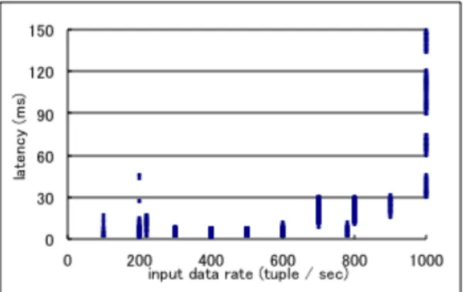
In this experiment, the threshold excess occurs when the measured latency violates 100 msec. This threshold was determined by conducting a series of experiments with varying
input data rate and measuring the obtained latency as shown in the following figure. The result is obtained by conducting 2000 keyword matching per tuple. Based on the obtained result shown in the following graph, we found out that the latency becomes very high and seemingly diverged when input data rate is 1000 tuples per second and more. In order to maximize the resource utilization, it would be better to choose the value which is very close to 1000 while avoiding the latency divergence. Thus, we decided to set the threshold to 100 msec in this experiment. This threshold value is not that changed if we change the number of keyword match to different value such as 1000.
26 tuples (0.13%) out of 21400 tuples exceeded the latency threshold with the T3 pattern. On the other hand, the CPU usage of T3 is relatively higher than others. It shows that the T1 and T2 patterns have too low load. In conclusion of this preliminary experiment, the Pattern T3, which has 2000 keyword matching, is an adequate processing load for our experiments since the CPU usage is relatively high and the latency average is kept low. Table 1: Performance Result with Different Keyword Matching Numbers
Pattern # of
keywords per one tuple
CPU usage average
Latency Average
Threshold Excess Number
Pattern T1 100 62.64 % 8.321 ms 0 / 21400 Pattern T2 1000 55.15 % 10.24 ms 0 / 21400 Pattern T3 2000 72.14 % 16.38 ms 26 / 21400
6.5 Comparison with Node Allocation Strategies
We test different node allocation strategies A1, A2, A3 and A4 each of which is described in Table 2, with Input Pattern T3 to check the effect of dynamic load balancing algorithm. Table 3 shows that the A2 and A3 allocation strategy cannot keep latency low.
The A2 allocation does not conduct any input data rate prediction. Thus when data streams comes at very high data rate, certain node is overloaded and its latency is diverged. Thus the threshold excess number becomes quite large since new node is added after the latency divergence is occurred.
The A3 allocation employs only the input data rate prediction algorithm and the node assignment is conducted in a round robin fashion. However this node assignment does not consider the status of each node whether it is busy or not. Thus when certain elapsed time
Input TupleNumber
elapsed time elapsed time
Input TupleNumber
Figure 2. # of Input Data Rate over Time
node is in a situation that it cannot handle more tasks, that node becomes overloaded.
The A4 allocation strategy extends the A3 allocation strategy by introducing two-level threshold for latency. The two-level threshold indicates that the first threshold means 100 msec in this example, and the second-level threshold might be 80 msec in this example. This strategy checks the status of all the nodes by obtaining the latency at each node. If the latency is close to the second-level threshold, the dynamic node allocation component decides not to allocate data to the node until the node becomes healthy. This solves the problem of the round-robin based scheduling that the A3 strategy takes. When dynamic load balancing module detects that the latency is too close to the threshold, it skips the node and then switch it to other nodes. The result in Table 3 shows the effectiveness of this strategy in that the threshold excess number is kept low. Also, the A4 allocation strategy outperforms other strategies in all the elements including the CPU utilization, the average latency, and threshold excess number. In conclusion of this experiments, it is found out that the A4 allocation strategy is the best strategy.
Table 2: Node Allocation Patterns Node Allocation Description Allocation A1
(Naïve)
4 nodes for System S,
4 nodes for Hadoop
Allocation A2 Dynamic load balancing w/o input data rate prediction
Allocation A3 Dynamic load balancing with input data rate prediction
Allocation A4 (Our approach)
Dynamic load balancing with input data rate prediction and latency
Table 3: Comparing Node Allocation Strategies Allocation CPU
usage
Latency average
Threshold excess number
Allocation A2 75.51 % 51.51 ms 7013 / 21400 Allocation A3 67.50 % 27.66 ms 1235 / 21400 Allocation A4 72.14 % 16.38 ms 26 / 21400
6.6 Comparing Our Proposed Allocation Strategy
with Naïve Node Allocation Strategy
In this section, we demonstrate that our best node allocation strategy (A4) outperforms naïve approach (A1).
6.6.1 CPU Utilization, Node Allocation and Latency
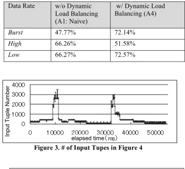
We compared the allocation strategy between A1 (naïve) with A4 (optimal). Allocation A1 does not use the function of IEP at all. Thus, it never causes the node switching and once the latency divergence occurs, there is no way to stop it. The input data rate illustrated in Figure 3 has a variety of data rates ranging from low to high, or sometimes in a burst situation. Figure 4 illustrates the time-series result with regards to the number of the running processes of System S as data stream processing with the IEP system. This result demonstrates that dynamic node allocation works properly by following the input data rate.
Table 4 shows the average of CPU usage rate of these experiments. It shows that Allocation A4 increases the CPU usage rate from 47.77% to 72.14% compared to the one with no load balancing at burst data rate. Moreover the result also shows the validity of the system at low data rate from 66.27 % to 72.57 %. However, load balancing algorithm does not show the advantage when the input data rate is high. This degradation comes from the fact that our current node allocation implementation allocates excessive node to System S. However this performance degradation needs to be further investigated.
The concluding result illustrated in Table 5 includes the comparison of the CPU Usage, Latency average, and threshold excess number at a burst situation. It demonstrates that our IEP system can increase the CPU usage while reducing the number of threshold excess. Another important point is that our system achieves the target goal described in Section 2.3 in that the average latency becomes relatively high while not violating the latency threshold (e.g. 100 msec in our scenario).
Table 4: Comparison of CPU Usage between Dynamic Load Balancing
Data Rate w/o Dynamic Load Balancing (A1: Naive)
w/ Dynamic Load Balancing (A4)
Burst 47.77% 72.14%
High 66.26% 51.58%
Low 66.27% 72.57%
Table 5: Comparing A1 and A4 Allocation CPU
usage
Latency average
Threshold excess number
Allocation A1 47.77 % 10.71 ms 121 / 21400 Allocation A4 72.14 % 16.38 ms 26 / 21400
elapsed time
Input TupleNumber
elapsed time elapsed time
Input TupleNumber
Figure 3. # of Input Tupes in Figure 4
elapsed time
Process Number
elapsed time elapsed time
Process Number
Figure 4. # of System S Processes with IEP
6.6.2 Throughput
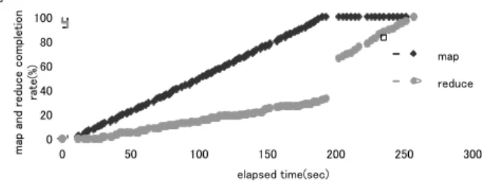
We also measured the effect on the throughput on batch processing with Hadoop. The throughput comparison can be done with the completion ratio of map and reduce tasks provided by the Hadoop daemon. Figure 6 illustrates the result that the Naïve allocation pattern (A1) which allocates 4 nodes to Hadoop. This experiment takes around 250 seconds to finish all the map/reduce tasks with 4 nodes, so the input data rate followed by Figure 5 that assumes 50 seconds, is continuously feeded 5 times. Figure 7 demonstrates the result of our IEP system (A4). As shown in both figures, the naïve approach finishes all the map/reduce tasks for around 250 seconds, whereas our approach finishes them for around 210 seconds. Both figures include the completion ration of map and reduce tasks. It has been observed that there is a jump of the completion ratio of reduce tasks but it depends on the Hadoop implementation, and is not the caused by our system. Since the IEP system provides dynamic node allocation depending on the input data rate, this result demonstrates that more nodes are allocated to Hadoop jobs when the data rate for System S is low, and then which leads to high throughput.
Figure 6. Hadoop Completion Time by Naïve Approach
Figure 7. Hadoop Completion Time with Dynamic Load Balancing
7. Related Work
David et. al proposes dynamic load balancing between several Web applications [12]. The granularity of these applications is variable, and some of these have dependencies on some computing nodes or need much computing resources. They construct and evaluate a framework which decides the most effective job allocation with less process migration. It is related to our work in a view point of dynamic load balancing, but it does not take care of the SLA (Service Level Agreement), which is the processing latency critically required for data stream processing.
Karve, et. al [13] describes a method of dynamic load balancing between transaction processing and batch processing. They assume many kinds of batch jobs. They differ in the granularity or CPU and memory loads. SLA of the processing latency is considered in this paper, and transaction processing is similar to Data Stream Processing because of the atomic process. However,
transaction processing is essentially finite while data stream processing includes infinite processes and continuous processing of incoming data from various sources. In addition, they only show theoretical results and do not provide any implementation and evaluation details of their system.
Zahalia, et al [17] proposed a job scheduling algorithm called delay scheduling to solve a conflict between fairness in scheduling and data locality when a data processing system such as Hadoop is shared by many users and hundreds of Hadoop jobs with various performance requirement are submitted. When the job that should be scheduled next according to fairness cannot launch a local task, it waits for a small amount of time, letting other jobs launch tasks instead. They implemented what is called the Hadoop Fair Scheduler that is a replacement of the default Hadoop’s FIFO based scheduler with delay scheduling. Their work is related to our work in a sense that they extended the default Hadoop system. However, our work is different in that our proposed system and scheduling policy puts higher priority to data stream applications in order to keep its SLA requirement rather than providing fairness to all the submitted jobs.
8. Concluding Remarks and Future Work
In this paper, we advocate an effective time series prediction algorithm for dynamic load balancing. We constructed and evaluated an Integrated Execution Platform for Data Stream Processing and Hadoop with the proposed algorithm. Our experimental result demonstrates that CPU usage is increased from 47.77% to 72.14% while keeping a low latency.
For future work, some improvement is needed for the load balancing algorithm and the time series prediction algorithm. A load balancing algorithm accounting the process switch time, dynamic index determination for SDAR and prediction algorithm using periodicity are needed.
Task switch system of Hadoop also needs improvements. At first, task switching should not be done by node but by CPU core. Second, the system needs to increase the HeartBeat Interval when the node has no task request in order to reduce the cost of HeartBeat. At last, task killing function is needed to reduce the wait time of switching.
We hope to evaluate this system with different input data patterns and other applications.
9. REFERENCES
[1] Daniel J Abadi, Yanif Ahmad, Magdalena Balazinska, Ugur Cetintemel, Mitch Cherniack, Jeong-Hyon Hwang, Wolfgang Lindner, Anurag S Maskey, Alexander Rasin, Esther Ryvkina, Nesime Tatbul, Ying Xing and Stan Zdonik, The Design of the Borealis Stream Processing Engine, CIDR 2005
[2] Chandrasekaran, Sirish and Cooper, Owen and Deshpande, Amol and Franklin, Michael J. and Hellerstein, Joseph M. and Hong, Wei and Krishnamurthy, Sailesh and Madden, Samuel R. and Reiss, Fred and Shah, Mehul A., TelegraphCQ: Continuous dataflow processing for an uncertain world, SIGMOD 2003
[3] Yousuke Watanabe and Hiroyuki Kitagawa, a Sustain-able Query Processing Method in. Distributed Stream Environment, the Database Society of Japan 2007
[4] Bugra Gedik, Henrique Andrade and Kun-Lung Wu, A Code Generation Approach to Optimizing High-
8
aai a%
a i
a
Performance Distributed Data Stream Processing, ACM 2008
[5] Bugra Gedik, Henrique Andrade, Kun-Lung Wu, Philip S. Yu and Myung Cheol Doo, SPADE : the System S declarative Stream Procesing Engine, SIGMOD 2008 [6] Lisa Amini, Henrique Andrade , Ranjita Bhagwan , Frank
Eskesen , Richard King , Yoonho Park and Chitra Venkatramani, SPC : a distributed, scalable platform for data mining, DMSSP 2006
[7] Joel Wolf, Nikhil Bansal, Kirsten Hildrum, Sujay Parekh, Deepak Rajan, Rohit Wagle, Kun-Lung Wu and Lisa Fleischer, SODA : An optimizing scheduler for large-scale stream-based distributed computer systems, Middleware 2008
[8] Yahoo, Apache Hadoop, http://hadoop.apache.org/
[9] Jeffrey Dean and Sanjay Ghemawat, Mapreduce: simplified data processing on large clusters, OSDI 2008.
[10] Yahoo Hadoop Tutorial, http://developer.yahoo.com/ hadoop/tutorial/module4.html
[11] Kenji Yamanishi and Jun-ichi Takeuchi, A unifying framework for detecting outliers and change points from non-stationary time series data, SIGKDD 2002
[12] Karve, A. and Kimbrel, T. and Pacifici, G. and Spreitzer, M. and Steinder, M. and Sviridenko, M. and Tantawi, A., Dynamic placement for clustered web applications, WWW 2006
[13] Carrera, David and Steinder, Malgorzata and Whalley, Ian and Torres, Jordi and Ayguade, Eduard, Enabling resource sharing between transactional and batch workloads using dynamic application placement, Middleware 2008
[14] Michael Isard, Mihai Budiu, Yuan Yu, Andrew Birrell, Dennis Fetterly: Dryad: distributed data-parallel programs from sequential building blocks. EuroSys 2007: 59-72 [15] Yuan Yu, Michael Isard, Dennis Fetterly, Mihai Budiu,
Úlfar Erlingsson, Pradeep Kumar Gunda, Jon Currey: DryadLINQ: A System for General-Purpose Distributed Data-Parallel Computing Using a High-Level Language. OSDI 2008: 1-14
[16] Matei Zaharia, Andy Konwinski, Anthony D. Joseph, Randy H. Katz, Ion Stoica: Improving MapReduce Performance in Heterogeneous Environments. OSDI 2008: 29-42
[17] Matei Zaharia, Dhruba Borthakur, Joydeep Sen Sarma, Khaled Elmeleegy, Scott Shenker, Ion Stoica: Delay scheduling: a simple technique for achieving locality and fairness in cluster scheduling. EuroSys 2010: 265-278 [18] Yong Zhao, Mihael Hategan, Ben Clifford, Ian T. Foster,
Gregor von Laszewski, Veronika Nefedova, Ioan Raicu, Tiberiu Stef-Praun, Michael Wilde: Swift: Fast, Reliable, Loosely Coupled Parallel Computation. IEEE SCW 2007: 199- 206
[19] Omer Ozan Sonmez, Nezih Yigitbasi, Alexandru Iosup, Dick H. J. Epema: Trace-based evaluation of job runtime and queue wait time predictions in grids. HPDC 2009: 111- 120
[20] Joao Pedro Costa, Pedro Martins, Jose Cecilio, and Pedro Furtado. 2010. StreamNetFlux: birth of transparent integrated CEP-DBs. In Proceedings of the Fourth ACM International Conference on Distributed Event-Based Systems (DEBS '10). ACM, New York, NY, USA, 101-102. [21] L. Neumeyer, B. Robbins, A. Nair, and A. Kesari. S4:
Distributed stream computing platform. In International Workshop on Knowledge Discovery Using Cloud and
Distributed Computing Platforms (KDCloud, 2010) Proceedings. IEEE, December 2010.