本文 Thesis 総合研究大学院大学学術情報リポジトリ A1906本文

(1)

Accelerated Star-Forming Activity before the

Peak Epoch as Revealed by Galaxies

Emitting Strong Lines of Doubly Ionized

Oxygen

SUZUKI TOMOKO

Doctor of Philosophy

Department of Astronomical Science

School of Physical Sciences

SOKENDAI (The Graduate University for

Advanced Studies)

定

(2)

(3)

Doctoral thesis

Accelerated Star-Forming Activity

before the Peak Epoch

as Revealed by Galaxies Emitting

Strong Lines of Doubly Ionized Oxygen

Department of Astronomical Science

School of Physical Sciences

The Graduate University for Advanced Studies

(SOKENDAI)

20140902

Tomoko Suzuki

Supervisor: Tadayuki Kodama

June 21, 2017

(4)

2

Abstract

The star-forming activity of galaxies in the Universe comes to its peak about ten billion years ago from the present-day Universe (redshift z ∼ 2). This epoch is called the “cosmic high noon”. In order to understand how the star-forming activity of galaxies is peaked towards the cosmic noon, we go further back in time to z ∼ 3–3.6 which is 1–2 Gyr prior to z ∼ 2. We aim to reveal what physical processes are involved in such a rapid increase of star formation rates (SFRs). So far, the ultraviolet (UV)-selected galaxies, such as Lyman Break Galaxies (LBGs), have been commonly used to probe the pre-peak epoch at z > 3. However, the UV-selected galaxies tend to be biased to bluer, less dusty star- forming galaxies due to strong dust extinction in the rest-frame UV regime. On the other hand, the rest-frame optical emission lines are less affected by dust extinction, and thus the optical emission line selected galaxies are more representing the star-forming galaxies including dusty ones. We focus on the [Oiii]λ5007 emission line instead of Hα to trace star-forming galaxies at z = 3–3.6 because Hα is no longer accessible at z > 2.6 from the ground. Recent studies have reported that high redshift normal star-forming galaxies tend to show strong [Oiii] emission as compared to the local counterparts. It is expected that we can use the [Oiii] emission line as a good tracer of star-forming galaxies at z > 3.

Imaging observation with a narrow-band (NB) filter, which can capture the redshifted strong emission lines from galaxies, is a powerful method to construct a sample of star- forming galaxies in a particular redshift slice. It provides us with a clean sample of star-forming galaxies down to a certain flux and equivalent-width (EW) limits. In this Thesis, we use the samples of NB-selected [Oiii] emission line galaxies at z > 3 obtained by the two systematic NB imaging surveys, namely Mahalo-Subaru and HiZELS.

In the first place, we want to confirm that the [Oiii] emitters actually trace star-forming galaxies at high redshifts with little bias. For this purpose, we compare [Oiii] emitters with Hα emitters at the same epoch (z = 2.23) selected NB filters at H and K-band, respectively. We find no significant difference on the global physical quantities between the two samples. This indicates that the [Oiii] emitters are not biased towards a particular population with respect to the Hα emitters at z = 2.23. We have thus confirmed that the [Oiii] emission line can be a useful tracer of star-forming galaxies at high redshifts.

With the [Oiii] emitters at z > 3 in the general fields, we investigate the star-forming

(5)

3 activity of galaxies before the peak epoch. Stellar masses and SFRs of the [Oiii] emitters show a positive correlation, which is known as the “main sequence” of star-forming galaxies. By comparing the M∗–SFR relation of the [Oiii] emitters with that of the NB-selected galaxies at z ∼ 2, we find that there is little evolution in the normalization of the main sequence between the two epochs, but that there is an offset along the constant main sequence towards the lower stellar masses with respect to the z ∼ 2 star-forming galaxies. Based on the assumption that the galaxies evolve along the constant sequence, we can estimate the stellar mass growth of star-forming galaxies from z = 3.2 to 2.2. As a result, a significant mass growth of galaxies during just 1 Gyr interval is suggested. Moreover, by dividing the samples at z = 3.2 and 2.2 into three stellar mass bins, we find that, from z = 3.2 to 2.2, the fraction of massive galaxies with relatively high sSFRs and high dust extinctions increases in the highest stellar mass bin. This suggests that the dusty star formation phase becomes more common among massive galaxies since z = 3.2 towards the peak epoch.

We also carried out the NIR spectroscopic observations of the [Oiii] emitters at z ∼ 3.24 with Keck/MOSFIRE. Comparing the excitation/ionization states and gaseous metallicities of the [Oiii] emitters at z ∼ 3.24 with those of other samples at the same epoch, we find that the [Oiii] emitters have similar ISM conditions to those of the UV continuum- selected galaxies, which are different from those of LAEs. We also compare the gaseous metallicities of the [Oiii] emitters with those of the star-forming galaxies at z ∼ 2 from the literature. Their gaseous metallicities are almost the same at a fixed stellar mass, and the mass–metallicity relation does not show a strong evolution between the two epochs.

In this Thesis, based on our unique NB-selected [Oiii] emitters, we investigate the physical properties of star-forming galaxies at z > 3. Our results infer that SFRs and gaseous metallicities are increased as their stellar masses grow along the constant scaling relations since z > 3. We also find that the fraction of massive galaxies in a dusty star formation phase is increased since z ∼ 3.2 to z ∼ 2.2, indicating a transition of the mode of star formation of some massive galaxies from a secular evolution phase to a dusty star formation phase. It is suggested that the star-forming activity of galaxies is accelerated since z > 3 towards the peak epoch. In order to reveal the physical mechanisms behind such a rapid galaxy growth, it is required to investigate their internal structures, kinematics, and molecular gas components with high resolution observations.

(6)

4

Acknowledgements

I am deeply grateful to my supervisor, Prof. Tadayuki Kodama for his continuous supports, encouragements, and comments/advices throughout the three years of my Ph.D. course. Without his guidance and invaluable helps, the completion of this thesis would not have been possible. I am also grateful to team members of Mahalo-Subaru and Ganba-Subaru project, Dr. Masao Hayashi, Dr. Yusei Koyama, Dr. Ken-ichi Tadaki, Dr. Ichi Tanaka, Dr. Yosuke Minowa, Rhythm Shimakawa and Moegi Yamamoto. They told me the basics of the optical/NIR observations, data reduction and analyses, and they always give me advices, comments, and helps.

I would like to thank collaborators from HiZELS team. I have received lots of helps and supports from Dr. David Sobral. Prof. Ian Smail, Prof. Phillip Best, and A. Khostovan gave me constructive comments and suggestions to complete my second paper.

I would like to thank Prof. Lisa Kewley for hosting me at the Mt. Stromlo Observatory for three months from October to December in 2015. I also want to thank her team members and the Faulkner court residents in Mt. Stromlo who helped me a lot during my stay. I had a great experience at Mt. Stromlo, and this experience leads me to think about going abroad as a researcher in the future.

I am grateful to Prof. Yoshiki Matsuoka, who recommended me for starting my Ph.D. course in NAOJ. Without his supports, I could not have made a decision to go into a new environment. I would like to thank Prof. Tsutomu Takeuchi, who supervised me when I was in the master course in Nagoya University, for his understanding.

I would like to acknowledge the financial support from SOKENDAI. It gave me oppor- tunities to stay Australia for three months, and to attend the international conferences many times.

I am really grateful to my friends in NAOJ, who have spent a lot of time together. Their encouragement always helps me. At last, I would like to show my heartfelt gratitude to my family for their continuous materially and mentally supports since I left my hometown.

(7)

List of figures

1.1 Cosmic star formation history . . . 10

1.2 Star-forming main sequence up to z ∼ 4 . . . 12

1.3 Mass–size relation and the redshift evolution of size . . . 14

1.4 Energy–level diagram for [Oiii] . . . 16

1.5 Stellar mass versus [Oiii]/Hβ ratio . . . 18

1.6 R₂₃-index versus [Oiii]/[Oii] ratio diagram . . . 19

2.1 NB filters on MOIRCS used in the observations at the SXDF . . . 29

2.2 Color–magnitude diagram for NB2095 . . . 30

2.3 Current status of Mahalo-Subaru project . . . 31

2.4 NB filters used in HiZELS . . . 32

3.1 Comparison of the redshift coverage between the NB_H (for [Oiii]λ5007) and NBK (for Hα) . . . 34

3.2 Comparison of SFRs derived from UV luminosities and Hα luminosities . . 42

3.3 Stellar mass–SFR relation of the Hα emitters and [Oiii] emitters at z = 2.23 43 3.4 Comparison of physical quantities between Hα emitters and [Oiii] emitters 44 3.5 Comparison of physical quantities between the three subsamples . . . 45

4.1 Color–color diagrams for NB2095 and NB2315 emitters . . . 51

4.2 Stellar mass versus SFR diagram with the selection limits . . . 52

4.3 Rest-frame U V J diagram . . . 53

4.4 Comparison of SFRs derived from the two different indicators . . . 55

4.5 Stellar mass–SFR relation of the Mahalo-Subaru [Oiii] emitters at z = 3.2–3.6 58 4.6 Stellar mass–SFR relation of the HiZELS [Oiii] emitters at z = 3.24 . . . . 63

4.7 Stellar mass–sSFR relation of the HiZELS [Oiii] emitters at z = 3.24 . . . . 64

4.8 Stellar mass–A_FUV relation of the HiZELS [Oiii] emitters at z = 3.24 . . . . 65 5

(12)

6

4.9 Number distribution of sSFR_UV and A_FUV . . . 66

4.10 Mass–size relation of the [Oiii] emitters at z = 3.2, 3.6 . . . 67

5.1 Redshift distribution of the [Oiii] emitters . . . 72

5.2 NIR spectra of the [Oiii] emitters . . . 73

5.2 continued . . . 74

5.2 continued . . . 75

5.3 Stacked spectra of the [Oiii] emitters . . . 76

5.4 Stellar mass–SFR diagram of the spectroscopically identified [Oiii] emitters 79 5.5 Comparison of SFRs derived from UV and Hβ . . . 81

5.6 Mass–excitation diagram . . . 82

5.7 R23-index versus [Oiii]/[Oii] for galaxies at z > 3 . . . 83

5.8 Metallicity versus line ratios (Maiolino et al., 2008) . . . 85

5.9 Metallicity versus line ratios (Curti et al., 2016) . . . 87

5.10 Mass–metallicity relation: empirical calibration . . . 90

5.11 Mass–metallicity relation: using the photoionization model . . . 91

5.12 FMR of the [Oiii] emitters . . . 92

6.1 Predicted stellar mass growth from z = 3.2 to z = 2.2 . . . 94

6.2 R₂₃-index versus [Oii]/[Oii] ratio : comparison with z ∼ 2 star-forming galaxies . . . 99

6.3 Mass–metallicity relation: comparison with z ∼ 2 star-forming galaxies . . . 99

6.4 Comparison with star-forming galaxies at z ∼ 2 on the FMR . . . 100

(13)

List of tables

3.1 Summary of NB filters in the H and K band used in HiZELS . . . 35

3.2 Summary of samples and subsamples used in this study. . . . 38

3.3 p-values from the KS-test: comparison between Hα emitters and [Oiii] emitters . . . 44

3.4 p-values from the KS-test: comparison of the three subsamples . . . 46

5.1 Summary of redshifts and emission line fluxes of the [Oiii] emitters . . . 77

5.2 Summary of the estimated physical quantities of the [Oiii] emitters . . . 80

5.3 Summary of metallicities and ionization parameters of the [Oiii] emitters estimated from the two metallicity calibration methods . . . 86

5.4 Summary of metallicities and ionization parameters of the [Oiii] emitters based on the photoionization models . . . 88

7

(14)

(15)

1 Introduction

1.1 Star formation history in the Universe

A galaxy is an astronomical object, which consists of a large collection of stars, interstellar gas, dust, and dark matter. From the cosmological context, galaxies are the fundamental units or “building blocks” that construct the large scale structures of the Universe. When we see the individual galaxies in the local Universe, however, galaxies themselves have different physical properties one another. They have different morphologies, colors, sizes, luminosities, stellar masses, star-forming activities, and so on. Investigating how the global properties of galaxies are changing with time and also how their great diversities are developing, will eventually lead us to understand how the galaxies are formed and evolved and how the galactic Universe is build-up with cosmic time down to the present- day.

The star-forming activity in the Universe are shown to have changed with cosmic time as in Figure 1.1 from Madau & Dickinson (2014). Going back in time from the present-day, the star formation rate (SFR) density increases monotonically up to 10 billion years ago or so. It reached to the peak activity at around 10–11 billion years ago corresponding to the redshift range of z ∼ 2–2.5. At higher redshifts, z ≳ 2.5, the SFR density turns over and starts decreasing towards the dawn of the Universe (e.g. Hopkins & Beacom, 2006; Madau & Dickinson, 2014). At z ∼ 1–3, the activities of active galactic nuclei (AGNs) are also known to be very high (Fan et al., 2004), indicating that the growth of the black- holes is also peaked in this redshift range. Such peak epoch of galaxy/AGN formation and evolution at z ∼ 1–3 is called the “cosmic noon”. Due to the very high star-forming activity of galaxies at the peak epoch, their physical properties are expected to be largely different from those of star-forming galaxies in the local Universe.

For investigations of high redshift galaxies, observations at the near-infrared (NIR) 9

(16)

10

Figure 1.1: The redshift evolution of star formation rate density from Madau & Dickinson (2014). SFR densities are estimated from the rest-frame far-ultraviolet and infrared measurements. The star-forming activity in the Universe is ∼ 10 times higher at z ∼ 1–3 (∼ 8–10 Gyr in lookback time) than z = 0.

wavelengths is very important as they can trace the light from stellar components of galaxies and can catch the important emission lines in the rest-frame optical (Section 1.4). There have been great progresses of the NIR instruments of the ground-based telescopes and the Hubble Space Telescope (HST ), and studies of high redshift galaxies have advanced substantially in recent years by the NIR photometric and spectroscopic observations. Our knowledge of physical states of those galaxies has been expanded significantly by many studies (e.g. Erb et al. 2006a; van Dokkum et al. 2008; F¨orster Schreiber et al. 2009; Kriek et al. 2009a; Wuyts et al. 2011; Genzel et al. 2014; Steidel et al. 2016).

1.2 Stellar mass–SFR relation of star-forming galaxies : the

“main sequence” of star-forming galaxies

One of the characteristic properties of star-forming galaxies at both low and high redshifts is a tight correlation between their stellar masses and SFRs (e.g. Brinchmann et al., 2004; Daddi et al., 2007; Elbaz et al., 2007; Noeske et al., 2007; Kashino et al., 2013). The positive correlation between the two quantities of star-forming galaxies is called the “main sequence” of star-forming galaxies (Figure 1.2 from Tomczak et al. (2016)).

(17)

11 A typical scatter of the observed sequence is ∼ 0.3 dex. Such a small scatter around the main sequence suggests that most of star-forming galaxies are forming stars via secular processes rather than violent processes, such as major mergers. Cosmological simulations propose a cold gas accretion from the outside of galaxies (e.g. Kereˇs et al., 2005; Kereˇs et al. , 2009; Dekel et al., 2009). Such a molecular gas inflow from outside would lead to a normal, secular star formation within galaxies. A scatter around the main sequence would reflect a difference of the gas accretion history among the individual galaxies, although there might be some observational uncertainties. On the other hand, galaxies in a starburst phase, which are usually very bright in the far-infrared (FIR), are distributed well above the main sequence (Elbaz et al., 2007; Daddi et al., 2007; Rodighiero et al., 2011).

While the scatter around the main sequence does not strongly evolve with redshift, the zero point of the relation strongly evolves with redshift to z ∼ 2 (e.g. Whitaker et al. 2012; Koyama et al. 2013; Tasca et al. 2015; Speagle et al. 2014; Tomczak et al. 2016). SFR increases monotonically with redshift at a given stellar mass (Figure 1.2), and SFRs of z ∼ 2 star-forming galaxies becomes ∼ 20 times higher than those of z ∼ 0 counterparts at a fixed stellar mass. From the observations of molecular gas components with CO emission lines, it has been revealed that higher SFRs of high redshift galaxies are primarily driven by their higher molecular gas fraction (e.g. Tacconi et al., 2010, 2013; Schinnerer et al., 2016). The star-forming activities of high redshift galaxies are thus expected to be higher according to the Schmidt-Kennicutt relation (Kennicutt, 1998a). The depletion time scales (inverse of the star formation efficiencies) are likely to change more slowly with redshift.

A redshift evolution of the star-forming main sequence has now been investigated even up to z ∼ 4 at least for massive galaxies (log(M∗/M⊙) > 10.0, e.g. Tasca et al. 2015; Speagle et al. 2014; Tomczak et al. 2016). At higher redshifts, it becomes more difficult to obtain a representative sample of star-forming galaxies down to a lower stellar mass regime. How SFRs at a fixed stellar mass (equivalent to specific star formation rates) evolve at z > 3 is still unclear mainly due to the incompleteness of samples of star-forming galaxies and the selection bias that it causes.

(18)

12

Figure 1.2: Stellar mass versus SFR diagrams for each redshift bin from z = 0.5 to z = 4.0 from Tomczak et al. (2016). In each redshift bin, a correlation between stellar masses and SFRs (the star-forming main sequence) is observed. Moreover, the bottom right panel shows a redshift evolution of the star-forming main sequence. Samples of star-forming galaxies are selected from the catalogs obtained by the ZFOURGE survey (Straatman et al., 2016). SFRs are estimated from a combination of the UV and IR luminosities.

1.3 Galaxy size and its dependence on stellar mass

The structural properties of galaxies, such as sizes and morphology, and the redshift evolution of such physical quantities are expected to reflect the mass assembly history of galaxies.

Galaxy sizes correlate with their stellar masses in the sense that massive galaxies have larger sizes than less massive galaxies at a particular redshift (left panel of Figure 1.3). It has been found that different galaxy populations, namely late-type (star-forming) galaxies and early-type (passive) galaxies, follow different mass–size relations. The sizes of early-type galaxies more strongly depend on their stellar masses as compared to those

(19)

13 of late-type galaxies (e.g. Shen et al., 2003; van der Wel et al., 2014; Allen et al., 2016a). The mass–size relation also changes with redshift as shown in Figure 1.3 from van der Wel et al. (2014). At a given stellar mass, galaxies are more compact at higher redshifts for both galaxy populations. Moreover, the average size evolution since z = 3 of early- type galaxies is more rapid than that of late-type galaxies. Such different size growth histories between the two populations suggests that some different physical mechanisms are involved in the mass assembly processes of early-type and late-type galaxies. The slow evolution of late-type galaxies may suggest a secular evolution of their sizes via internal star formation.

The redshift evolution of the sizes of star-forming galaxies has been investigated up to z ∼ 7 or even higher redshifts using the LBGs or mass-selected samples (e.g. Mosleh et al., 2012; Shibuya et al., 2015; Allen et al., 2016b). These results all suggest that the sizes decreases with redshifts, however, the slopes of the size evolution are slightly different among the different studies probably due to the different methods of size measurements and different sample selections. We here note again that, in particular at z > 3, it is critical to obtain a representative sample of star-forming galaxies in a narrow redshift range.

At higher redshifts, it is more difficult to measure the accurate sizes of galaxies because their sizes become smaller with redshifts and the wavelength range that can neatly trace the underlying stellar components in mass becomes redder and redder with redshift. Therefore we need to obtain higher angular resolution images of high redshift galaxies at the NIR wavebands (or even longer wavelengths if possible). The Wide Field Camera 3 (WFC3) on the HST is a powerful instrument for this purpose. The WFC3/H-band can capture the rest-frame optical light from high redshift galaxies at least up to z ∼ 3 or so.

On the mass–size relation especially for high redshift galaxies, massive and compact early-type galaxies are often found. Such compact quiescent galaxies are one of the most characteristic objects at high redshift Universe, and they are called “red nuggets” (e.g. Daddi et al. 2005; Damjanov et al. 2009; van Dokkum et al. 2010). Recently, their likely progenitors, namely, compact and massive star-forming galaxies, are also commonly observed at high redshifts (e.g. Barro et al. 2013). The compact star-forming galaxies are though to be formed by gas-rich processes such as mergers or disk instabilities that invoke starbursts in the central compact regions. They would then become compact, quiescent

(20)

14

Figure 1.3: Two figures related to the galaxy size evolution from van der Wel et al. (2014). (Left) : Mass–size relation of the late-type (blue dots) and early-type (red dots) galaxies in each redshift bin. The solid lines represent the model fits to the early-type and late-type galaxies of each redshift bin, and the dashed lines represent the model fits to the galaxies at 0 < z < 0.5. The relations between stellar masses and sizes are totally different between the two galaxy populations in any redshift bins.

(Right) : The redshift evolution of the size at the fixed stellar mass of 5 × 10¹⁰M⊙. Blue and red dots show late-type and early-type galaxies, respectively. The size evolution of the late-type galaxies since z = 3 is relatively slow as compared to that of the early-type galaxies.

galaxies when their star formation is quenched (Barro et al., 2013). The cosmic noon and the epoch before the cosmic noon are critical for us to study and reveal the evolutionary path from the compact star-forming galaxies to the compact quiescent galaxies.

1.4 Interstellar medium conditions of star-forming galaxies

1.4.1 Emission lines from the ionized gas

In a star-forming region within a galaxy, hot, young, and massive stars (OB-type stars) are embedded. By strong ionizing fluxes from the OB stars, the hydrogen atoms and metals are ionized and a Hii region is formed around massive stars. Various emission lines are observed in the spectra emitted from Hii regions. There are emission lines from various atoms in different ionization states, and their relative strengths depend on the physical

(21)

15 conditions of the surrounding region, such as metallicities, electron densities, hardness of ionizing photons, and so on (e.g. Kewley & Dopita, 2002; Kewley et al., 2013; Steidel et al., 2016).

The strength of emission lines from ionized gas is basically correlated with SFR, and therefore the emission lines (not all of the emission lines) from Hii regions are used as indicators of star-forming galaxies (e.g. Bunker et al. 1995; Malkan, Teplitz & McLean 1996; Sobral et al. 2013; Hagen et al. 2015). Among the various emission lines across a wide wavelength range, the emission lines in the rest-frame optical have been commonly used to trace star-forming galaxies and estimate their physical quantities. For example, the Hα emission line at 6563 ˚A is one of the best indicators of star-forming galaxies because it is strong and less affected to dust extinction than the UV light, and the relation between SFRs and Hα luminosities has been well calibrated in the local Universe (e.g. Hopkins et al. 2003). Moreover, the ratio of Hα and Hβ (4861 ˚A) or Hβ and Hγ (4340 ˚A) is frequently used to determine the amount of dust extinction (Osterbrock & Ferland, 2006).

Oxygen is a relatively common metal in the Universe. The forbidden lines of doubly ionized oxygen ([Oiii]) and singly ionized oxygen ([Oii]) are observed in the spectra of Hii regions. In the rest-frame optical spectra, there are strong emission lines of oxygen, namely, [Oiii]λλ5007,4959 and [Oii]λ3726,3729. These emission lines are collisional excitation lines, and therefore, the strengths of [Oiii] and [Oii] largely depends on the conditions of ISM in contrast to the Balmer lines, such as Hα and Hβ.

For example, when the ionization parameters, the ratio of the number density of ionizing photos to that of hydrogen atoms (see Section 1.4.2 for the definition), are high, the ionization of O⁺ to O⁺⁺ is facilitated. As a result, the [Oiii] emission becomes stronger with respect to the [Oii] emission. Lower gaseous metallicities make gaseous temperature high due to the lack of gas coolants. High gaseous temperatures enhance the collisional excitation lines with respect to a recombination line of hydrogen. Additionally, when the ionizing spectra become harder, the enhancement of the collisional excitation is seen because the kinematic energy of ionized spectra becomes larger (Kewley & Dopita, 2002; Strom et al., 2016).

(22)

16

Figure 1.4: Schematic view of the energy–level diagram for lowest terms of [Oiii]. The emission lines in the optical wavelength are represented as the solid lines. Those in the UV wavelength are represented as the dashed lines. In our study, we focus on the [Oiii]λ5007 emission line.

1.4.2 Different physical conditions of high redshift star-forming galaxies

The ISM conditions of galaxies are described by gaseous metallicities, ionization parameters, electron densities, ionizing spectra, and so on (Kewley et al., 2013; Masters et al., 2014; Nakajima & Ouchi, 2014; Onodera et al., 2016). An (effective mean) ionization parameter q is defined as follows:

q ≡ ^Q^H⁰

4πR²_sn^, ^(1.1)

where Q_H⁰ is the flux of the ionizing photons produced by the existing stars above the Lyman limit, Rs is the Str¨omgren radius, and n is the local number density of hydrogen atoms (Kewley & Dopita, 2002). Simply stated, the ionization parameter is the ratio of a density of ionizing photons to that of hydrogen atoms at the surface of a Hii region.

For example, gaseous metallicities is determined by the contributions from star formation and gas inflow/outflow processes. Ionization parameters are determined by the compactness of star-forming regions and/or the strength of the ionizing source. Spectrum shapes (hardness) of ionizing photons depend on the stellar populations in a star-forming

(23)

17 region. The ISM conditions of galaxies are thus closely related to their star-forming activity, and it is expected that at higher redshifts, where galaxies are forming stars more actively, galaxies are expected to have different ISM conditions from local star-forming galaxies.

Recently, some large NIR spectroscopic observations have been carried out, such as KBSS-MOSFIRE (Steidel et al., 2014) and MOSDEF (Kriek et al., 2015). From NIR spectra of high redshift star-forming galaxies, the extreme ISM conditions of star-forming galaxies are suggested (e.g. Masters et al. 2014; Steidel et al. 2014; Shapley et al. 2015; Holden et al. 2016). One is an offset on the Baldwin-Phillips-Terlevich (BPT) diagram (Baldwin, Phillips & Terlevich, 1981). High redshift galaxies show a high [Oiii]/Hβ ratio at a fixed [Nii]/Hα ratio with respect to the sequence of local star-forming galaxies (e.g. Masters et al., 2014; Steidel et al., 2014; Shapley et al., 2015; Kashino et al., 2016). Another is the higher [Oiii]/Hβ ratios of high redshift galaxies than the local galaxies at a fixed stellar mass as shown in Figure 1.5 (e.g. Shimakawa et al., 2015; Holden et al., 2016; Strom et al., 2016).

Figure 1.6 shows the R₂₃-index versus [Oiii]/[Oii] ratio diagram. R₂₃-index represents the ratio of ([OIII]λλ5007, 4959 + [OII]λ3727)/Hβ. Although the R23-index and [Oiii]/[Oii] ratio depend on both metallicity and ionization parameter, R₂₃-index is more sensitive to the metallicity, while the [Oiii]/[Oii] ratio is more sensitive to the ionization parameter (Kewley & Dopita, 2002). Using the two line ratios, Nakajima & Ouchi (2014) discussed the metallicity and ionization parameter simultaneously for high redshift LBGs and LAEs (Figure 1.6). On the R₂₃-index versus [Oiii]/[Oii] ratio diagram, high redshift star-forming galaxies are distributed on the region of higher R₂₃-index and higher [Oiii]/[Oii] ratio (e.g. Nakajima & Ouchi 2014; Shapley et al. 2015; Onodera et al. 2016; Strom et al. 2016), where metal-poor galaxies at z = 0 are distributed. High redshift galaxies tend to show higher ionization parameters and lower gaseous metallicities sys- tematically. Higher R₂₃-indices of high redshift star-forming galaxies are also explained by the harder ionizing radiation fields (Steidel et al., 2016; Strom et al., 2016).

We note that there might be a kind of selection effect to the results that the high redshift star-forming galaxies have extreme ISM conditions. Juneau et al. (2014) showed that the local galaxies that are selected with a certain detection limit of emission line at high redshifts tend to show higher [Oiii]/Hβ ratios on the BPT or Mass–Excitation

(24)

18

Figure 1.5: Relation between stellar mass and [Oiii]/Hβ ratio (Mass–Excitation diagram, Juneau et al. 2011) of z > 3 Lyman Break Galaxies (LBGs) from Holden et al. (2016). Filled circles show their LBG sample, and the filled triangles and open circles represent the LBG samples at z > 3 from the literature. The local galaxies from SDSS are shown in the grayscale. In the top panel, the contours show the two branches of the star-forming galaxies and AGNs.

diagram as observed for the star-forming galaxies at z ∼ 1.5. If fainter emission line galaxies at high redshifts below the limits were included, the ISM conditions of star- forming galaxies would not strongly evolve with redshift (e.g. Juneau et al., 2014; Dickey et al., 2016).

1.4.3 Mass–metallicity relation across cosmic time

As mentioned above, a gaseous metallicity¹ is an important physical quantity of galaxies. There are some calibration methods to measure the gaseous metallicity of galaxies.

One is called a “direct electron-temperature (Te) method” (e.g. Izotov et al. 2006; An- drew & Martini 2013; Kojima et al. 2016; Sanders et al. 2016b). The ratios of the strong line and auroral line of the same ions, for example, [Oiii]λλ5007,4959 and [Oiii]λ4363 (Figure 1.4), are sensitive to the electron temperature of the ionized gas. Since metals in gas phase are major coolants of Hii regions, electron temperatures correlate with gaseous metallicities (abundance of a particular ion), and therefore, we can measure gaseous metal-

1Throughout this Thesis, a “gaseous metallicity” usually means a gaseous oxygen abundance, 12+log(O/H).

(25)

19

Figure 1.6: The relation between R23-index and [Oiii]/[Oii] ratio from Nakajima & Ouchi (2014). The LBGs and LAEs at z = 2–3 are represented with the blue symbols and the red symbols, respectively. The gray scale represents the local SDSS galaxies.

licities by obtaining electron temperatures and electron densities. However, since the auroral lines are very weak, it is difficult to detect the auroral lines for individual galaxies especially for metal-rich galaxies and at high redshifts.

To date, various metallicity calibration methods using relatively strong emission lines, which are easier to observe, are proposed by many studies. Some studies empirically calibrate relations between the line ratios and metallicities, which are estimated from the direct Te method (e.g. Pettini & Pagel 2004; Maiolino et al. 2008; Jones et al. 2015; Curti et al. 2016). These relations are calibrated with the star-forming galaxies at z = 0. Some studies calibrate relations between the line ratios and metallicities based on the photoionization models of Hii regions (e.g. Kewley & Dopita, 2002; Kobulnicky & Kewley, 2004; Dopita et al., 2016). Kewley & Ellison (2008) showed that gaseous metallicities which are estimated with different calibrations tend to show systematic offsets one another. Therefore, we have to keep it mind when we compare the gaseous metallicities estimated with different methods.

The correlation between stellar masses and gaseous metallicities of star-forming galaxies is called the mass–metallicity relation. Mass–metallicity relations have been investigated from z = 0 to z > 3 (e.g. Tremonti et al. 2004; Erb et al. 2006a; Maiolino et al.

(26)

20

2008; Zahid et al. 2014; Steidel et al. 2014). Gaseous metallicities of star-forming galaxies at a fixed stellar mass decrease with redshift, which is more prominent for less massive galaxies (Zahid et al., 2014). However, due to the discrepancy between metallicity calibration methods and the low signal-to-noise ratios of spectra of high redshift galaxies, the redshift evolution of the mass–metallicity relation is still under debate especially at higher redshifts (z > 2).

The scatter of the mass–metallicity relation is large in contrast to that of the stellar mass–SFR relation. Mannucci et al. (2010) showed that there is a correlation between the metallicities and SFRs. Star-forming galaxies with lower SFRs tend to have lower metallicities at a given mass, and the local SDSS galaxies are distributed on a surface in the three-dimensional space of stellar mass, SFR, and metallicity. This is called the fundamental metallicity relation (FMR). In Mannucci et al. (2010), they introduced µα, which is defied as µ_α = log(M∗) − α × log(SFR). The α value is chosen to be 0.32 so that the scatter around the projected FMR on the 12+log(O/H) versus µα plane can be minimized. Not only the local galaxies, but also the star-forming galaxies up to z ∼ 2.5 are claimed to follow the same FMR, while there are some other studies which show weak correlations between gaseous metallicities and SFRs at z ∼ 2 (e.g. Wuyts et al., 2014; Cullen et al., 2014; Strom et al., 2016).

1.5 Going back in time before the peak epoch with the [Oiii]

emission line

In order to understand how and why the star-forming activity increases towards the peak epoch at z ∼ 1–3, it is necessary to go further back in time before the peak epoch, i.e. z > 3. The epoch of z = 3–3.6 corresponds to just 1–2 Gyr before the highest peak.

To date, samples of galaxies at z > 3 are mainly constructed by tracing the UV light from hot, young, and massive stars in star-forming regions. Since the UV light is strongly affected by the dust extinction, the UV-selected galaxies tend to be biased towards younger and bluer star-forming galaxies (Cowie et al., 2011). In terms of the insensitivity to the dust extinction, the rest-frame optical emission lines are useful as mentioned in Section 1.4.1. Emission lines at shorter wavelengths than Hα are accessible at z > 3 from the ground.

(27)

21 In this Thesis, we will focus on the [Oiii]λ5007 emission line instead of Hα to trace the star-forming galaxies at z ∼ 3–3.6. As mentioned in Section 1.4.2, it is has been revealed that the high redshift star-forming galaxies tend to show higher [Oiii]/Hβ ratios compared to the local counterparts (Steidel et al., 2014; Shapley et al., 2015; Holden et al., 2016). It is easier to observe [Oiii] emission lines from galaxies even at z > 3 than Hβ or [Oii], for example. We expect that [Oiii]λ5007 emission line can be a useful tracer of star-forming galaxies at z > 3.

On the other hand, there are possible biases emerging by using [Oiii] as an indicator of star-forming galaxies. One is related to the contribution of AGNs. The [Oiii] emission line originates from the gas ionized not only by hot, young massive stars in the star-forming regions but also by central AGNs (Zakamska et al., 2004). At least in the local Universe, strong [Oiii] emission is often regarded as an evidence for the presence of AGN. Galaxies traced by their strong [Oiii] emission are likely to be more contributed by AGNs compared to the galaxies traced by other emission lines.

Because of the slightly shorter wavelength of the [Oiii] line (5007˚A) with respect to the Hα line (6563˚A), the samples of [Oiii]-selected galaxies may be inherently biased against dusty systems in comparison to the Hα-selected samples, although the dust extinction at the wavelength of the [Oiii] emission line is only ∼ 1.3 times larger than that at the wavelength of the Hα emission line based on the extinction curve of Calzetti et al. (2000). Moreover, the strength of [Oiii] emission line is sensitive to the physical conditions of the ISM as mentioned in Section 1.4.1. Galaxies traced by [Oiii] emission might be biased towards galaxies with lower stellar masses given the well-known mass–metallicity relation of star-forming galaxies.

Therefore, before we carry out a systematic survey of star-forming galaxies at z ∼ 3–3.6 with [Oiii] emission lines, it is necessary for us to confirm the usefulness of the [Oiii] emission line as an indicator of star-forming galaxies at high redshifts.

1.6 This Thesis

In this Thesis, we focus on the galaxy formation before the peak epoch, and construct the samples of star-forming galaxies at z > 3 by capturing their [Oiii] emission lines by narrow-band (NB) filters. We here use the NB imaging data obtained by the two NB

(28)

22

surveys, namely Mahalo-Subaru and HiZELS. In Chapter 2, we introduce the selection method of star-forming galaxies from the NB imaging data.

In Chapter 3, in the first place, we investigate the usefulness of the [Oiii] emission line as a tracer of star-forming galaxies at high redshifts. We compare the physical quantities of the [Oiii]-selected galaxies at z = 2.23 with those of the Hα-selected galaxies at the same redshift in the COSMOS field obtained by HiZELS.

In Chapter 4, we investigate the star-forming activity of the [Oiii] emitters at z > 3. We use the two samples of [Oiii] emitters in the general fields at z = 3.18, 3.63 and z = 3.24 obtained by Mahalo-Subaru and HiZELS, respectively. We estimate SFRs from the UV luminosities and investigate the relation between the stellar mass and SFR of the [Oiii] emitters at z > 3. Then, we compare the stellar mass–SFR relation at z > 3 with that of the NB-selected galaxies at z ∼ 2. For the [Oiii] emitters obtained by Mahalo-Subaru, we measure the sizes of galaxies using their H-band images taken with the HST/WFC3. We investigate the relations between the stellar mass and size of the star-forming galaxies at z > 3. For the [Oiii] emitters obtained in HiZELS, taking an advantage of the large number of available sources, we divide the samples at z = 3.24 and z = 2.23 into three stellar mass bins. We compare the specific SFR and dust extinction of the star-forming galaxies with comparable stellar masses between the two epochs.

In order to investigate more detailed physical conditions, we carry out a NIR spectroscopic observation for the [Oiii] emitters at z = 3.24 with Keck/MOSFIRE. In Chapter 5, we show the observational results of the NIR spectroscopy and discuss the ISM conditions of the [Oiii] emitters by comparing them with other galaxy populations at the same epoch. We measure gaseous metallicities of the [Oiii] emitters using three calibration methods, and investigate the relation between their stellar masses and metallicities, and the correlation between the metallicities and SFRs.

In Chapter 6, we discuss the galaxy growth from z > 3 towards the peak epoch at z ∼ 2 based on our results obtained in Chapter 4. Moreover, we discuss the redshift evolution of the ISM conditions of star-forming galaxies. We compare our [Oiii] emitters at z ∼ 3.24 with the sample of star-forming galaxies at z ∼ 2.2 in the literature on the R₂₃-index versus [Oiii]/[Oii] ratio diagram and on the mass–metallicity diagram.

In Chapter 7, we summarize our study, and in Chapter 8, we address future observational plans using the [Oiii] emitters at z ∼ 3–3.6.

(29)

23 Throughout this Thesis we assume the cosmological parameters of Ω_m= 0.3, Ω_Λ = 0.7, and H₀ = 70 kms⁻¹Mpc⁻¹, unless otherwise noted. All the magnitudes are given in AB system (Oke & Gunn, 1983).

(30)

(31)

2 Selection methods of star-forming

galaxies based on NB imaging

2.1 Imaging observation with NB filters and its advantages

As mentioned in Section 1.4.1, the ionized regions by hot, young, and massive stars emit various emission lines, such as Hα, [Oiii], Hβ, [Oii], Paα, and so on. We can catch the redshifted emission lines by imaging observations with a NB filter. This is one of the most powerful methods to construct a sample of star-forming galaxies at a particular redshift slice (e.g. Bunker et al. 1995; Malkan, Teplitz & McLean 1996; Moorwood et al. 2000; Geach et al. 2008). By taking the images not only with a NB filter, but also with a broad- band (BB) filter corresponding to the wavelength of the NB filter, we can pick up the NB excess sources, which are brighter in NB than BB. We can also estimate fluxes of an emission line for the NB emitters from the NB and BB data as explained in Section 2.2.

NB excess sources consist of different emission line galaxies at different redshifts. Once we identify redshifts of NB emitters by using their colors or photometric redshifts (see Section 2.2 for more details), we can obtain a sample of emission line galaxies at a particular redshift range. A redshift range of galaxies picked up by a NB imaging is much narrower than that of galaxies obtained by BB color selections, such as the BzK selection (e.g. Daddi et al. 2005) or the Lyman break selection (e.g. Steidel & Hamilton 1997). Moreover, since the NB selection is based on the emission line fluxes and EWs, we can obtain a nearly SFR-limited sample of star-forming galaxies within a narrow redshift range. This is also one of the advantages of the NB imaging observation.

We also note that the high efficiency of follow-up observations for the NB-selected galaxies. As mentioned above, since the redshifts and emission line fluxes are already

25

(32)

26

known from the NB imaging observations, the feasibility of observations, such as line diagnostic spectroscopy and integral field unit (IFU) spectroscopy, becomes very high.

The star-forming galaxies used in this Thesis is selected based on the NB technique. In the following, we briefly introduce an example to show how the emission line galaxies are selected from the obtained NB data, and how we can estimate the line fluxes of the emitters.

2.2 Selection methods of NB emitters and flux measure-

ment

The observational data introduced in this Section as an example are obtained by the NB imaging observations with the Multi Object InfraRed Camera and Spectrograph (MOIRCS; Suzuki et al. 2008) on the Subaru telescope. The target field is the Subaru/XMM- Newton Deep survey Field (SXDF; Furusawa et al. 2008). The two NB filters, namely NB2095 (λc = 2.093 µm, FWHM = 0.026 µm) and NB2315 (λc = 2.317 µm, FWHM = 0.026 µm), are used (Tadaki et al., 2013). Figure 2.1 shows the transmission curves of the two NB filters. We introduce the case of NB2095 below, and the details of the observations and the data reduction are described in Tadaki et al. (2013).

First of all, we extract sources from the NB images taken with MOIRCS and the BB (H and K bands) images taken with the Wide Field Camera (WFCAM; Casali et al. 2007) on the United Kingdom Infrared Telescope (UKIRT), using the public software SExtractor (Bertin & Arnouts, 1996). The pixel scales and PSF sizes of the BB images are matched to those of the NB images. We perform aperture photometries on the NB and BB images with a 1^′′.6 diameter aperture. Source extraction and photometries are carried out with the double image mode of SExtractor. Those aperture photometry data are used to select line emitters based on the color–magnitude diagram as shown in Figure 2.2.

The sources which are much brighter in NB as compared to BB are selected as the line emitters. Since the effective wavelengths of the NB filter and the K-band are slightly different (Figure 2.1), we estimate the BB fluxes at the exact effective wavelengths of the NB2095 filter by interpolating fluxes between H and K bands as follows (Tadaki et al., 2013):

(33)

27

HK(λ = 2.09 µm) = 0.8 K + 0.2 H − 0.015. (2.1) We select NB excess sources using HK −NB2095 color versus NB 2095 magnitude diagram (Figure 2.2). Here we set the three selection criteria. The first criterion is that the NB magnitude is brighter than the 5σ limiting magnitude (m_NB,5σ = 23.6mag; the vertical dashed line in Figure 2.2).

The second criterion is based on the selection using a parameter Σ, which determines the significance of an NB excess relative to a 1σ photometric error (Bunker et al., 1995). The relation between Σ and the color of mBB− mNB is obtained from

m_BB− m_NB= −2.5 log₁₀



1 −^Σ

√

σ_BB² + σ_NB² fNB



, (2.2)

where f_NBis a NB flux density, σ_BB² and σ²_NBare the sky noises in the BB and NB images measured within an aperture, respectively (Tadaki et al., 2013). We set the criterion of Σ = 3 to sample secure emitters, and it is represented as the solid curve in Figure 2.2. This selection criterion corresponds to the limit of the emission line flux. For this observation with NB2095, the line flux limit at the 3σ significance level is F_line = 1.5 × 10⁻¹⁷erg s⁻¹cm⁻².

The third one is HK − NB > 0.4 mag, which determines the NB magnitude excess with respect to the HK magnitude (the horizontal solid line in Figure 2.2). This selection criterion corresponds to the limit of the EW of EW_rest> 30 ˚A for the [Oiii] emitters at z=3.18.

The NB and BB flux densities are defined as

f_NB= fc+ F_line/∆_NB, (2.3)

f_BB= fc+ F_line/∆_BB, (2.4)

where fc is a continuum flux density, F_line is a line flux intensity, and ∆_NB and ∆_BB are FWHMs of the NB and BB filters (Tadaki et al., 2013). The continuum flux density, the line flux intensity, and the EW in the rest-frame are given by the following equations, respectively;

(34)

28

fc = ^f^BB^{− f}^NB^(∆^NB^/∆^BB⁾ 1 − ∆NB/∆BB

, (2.5)

F_line= ∆_NB ^f^NB^{− f}^BB

1 − ∆_NB/∆_BB^, ^(2.6)

EW_rest= ^F^line

f_c ^{(1 + z)}

−₁

. (2.7)

The NB excess sources selected by the color–magnitude diagram consist of different emission line galaxies at different redshifts. In the case of NB2095, Paα emitters at z = 0.12, Hα emitters at z = 2.19, [Oiii] emitters at z = 3.18, and [Oii] emitters at z=4.61 are possibly included in the emitter sample. When separating their redshifts, the multi- wavelength photometry is required. The color–color diagrams or photometric redshifts are often used to identify the redshifts of the NB emitters (e.g. Hayashi et al. 2012; Sobral et al. 2013). When we try to separate the redshifts of galaxies with the color–color diagram, for example, the conspicuous spectral features such as the Balmer and/or 4000˚A breaks or the Lyman break can be used. Since the break feature is redshifted to a different wavelength in the observed frame according to the redshifts of galaxies, by choosing an appropriate combination of passbands that can neatly straddle the spectral break feature, we are able to disentangle the various possible solutions for different line emitters at different redshifts. We do not require a high accuracy for these selection methods because the possible emitters have largely different redshift ranges with each other.

2.3 Mahalo-Subaru

“Mahalo-Subaru” (MApping HAlpha and Lines of Oxygen with Subaru; Kodama et al. 2013) is a systematic NB imaging survey with the Subaru Prime Focus Camera (Suprime- Cam; Miyazaki et al. 2002) and MOIRCS on the Subaru Telescope. This project aims to reveal the emergence of the environmental dependence of galaxy properties in the history of the Universe by targeting high density regions, such as galaxy clusters/proto-clusters, as well as the lower-density blank fields, and constructing a coherent sample of NB-selected star-forming galaxies across various environments and cosmic time (Figure 2.3).

So far, this project focuses on star-forming galaxies mainly at z ∼ 1–2.5. For example, in Hayashi et al. (2012) and Koyama et al. (2013), they targeted Hα emitters residing

(35)

29

Figure 2.1: Transmission curves of the K-band filter on UKIRT/WFCAM (dotted line), and the two NB filters on MOIRCS, namely NB2095 and NB2315, used in the NB imaging observation at the SXDF (solid lines). With the NB filters, we capture the emission lines from the distant galaxies. K-band data are used to estimate the stellar continuum (Section 2.2).

in proto-cluter environments at z ∼ 2.5 and 2.2, respectively. Their results suggest the presence of the active star-forming galaxies in rich environments as contrasted to galaxy clusters at lower redshifts. Tadaki et al. (2013, 2014) carried out z ∼ 2 Hα emitter survey with MOIRCS in the SXDF. They constructed a sample of star-forming galaxies at z = 2.2 and 2.4 using the two NB filters, namely NB2095 and NB2315. The HST images are available for all the Hα emitters. They found the clumpy structures of the Hα emitters at z ∼ 2, and that the redder star-forming clumps tend to be near the center of galaxies, indicating the bulge formation accompanied by dusty star formation in the central region of normal star-forming galaxies.

Now, we are expanding our survey to more distant Universe, i.e. z > 3, in order to investigate the galaxy formation and its environmental dependence before the peak epoch. So far, as a field sample, we have constructed a sample of [Oiii] emitters at z = 3.18 and 3.62 in the SXDF. These [Oiii] emitters are obtained from the same observational data shown in Tadaki et al. (2013, 2014). We will explain the details of this sample in Chapter 4. Also, we have already carried out the [Oiii] imaging observation in a proto-cluster environment at z = 3.13, namely MRC0316-257 (Venemans et al., 2007), with MOIRCS

(36)

30

Figure 2.2: Color–magnitude diagram for NB2095. Gray dots represent all the sources detected in the NB images, and blue filled circles are the sources selected as the NB emitters with our selection criteria. The solid curve correspond to ± 3σ photometric errors, and the horizontal red line corresponds to HK − NB = 0.4 [mag]. The vertical dashed line corresponds to the 5σ limiting magnitude of the NB2095 data.

and NB2071 filter. [Oiii] imaging observations in proto-cluster fields at z > 3 are one of the future prospects of this Thesis. We will touch on this again in Chapter 8.

2.4 HiZELS

HiZELS, the High-Z Emission Line Survey (Best et al., 2013; Sobral et al., 2013), is a panoramic NB imaging survey using NB filters in the J, H, and K bands of WFCAM on UKIRT, and the NB921 filter of the Suprime-Cam on the Subaru telescope (Figure 2.4). Their main survey fields are the general fields, such as the Cosmological Evolution Survey (COSMOS) field (Scoville et al., 2007) and the UKIDSS Ultra Deep Survey (UDS) field (Lawrence et al., 2007).

HiZELS covers a wide field-of-view, for example, ∼ 1.6 deg² in the COSMOS field. With the large number of emitters ([Oii], [Oiii], and Hα emitters) at various redshifts, the clustering properties of emitters, the redshift evolution of the emission line and luminosity function, stellar mass function, and SFR function has been investigated (e.g. Geach et al.

(37)

31

Figure 2.3: The current status of Mahalo-Subaru project (Credit: Tadayuki Kodama).

2008; Sobral et al. 2013, 2014; Khostovan et al. 2015, 2016).

The catalogs of the emitters obtained by their four NB filters are now publicly available (Sobral et al., 2013), and they have constructed samples of [Oiii] emitters at z = 0.84, 1.42, 2.23, and 3.24 (Khostovan et al., 2015). In this Thesis, we use the NB emitter catalogs from HiZELS as well as those of our own project, Mahalo-Subaru.

(38)

32

Figure 2.4: The transmission curves of the BB and NB filters used in HiZELS (Sobral et al., 2013). The NB filters in the z^′ (Subaru/Suprime-Cam), J, H, and K-bands (UKIRT/WFCAM) catch the redshifted Hα line at z = 0.40, 0.85, 1.47, and 2.23, and [Oiii]λ5007 line at z = 0.84, 1.42, 2.23, and 3.24, respectively, for example (Sobral et al., 2013; Khostovan et al., 2015).

(39)

3 [Oiii] emission line as a useful

tracer of star-forming galaxies

at high redshifts

The Hα emission line is one of the best tracers of star formation because it is less affected to dust extinction than the UV light and the relation between SFRs and Hα luminosities has been well calibrated in the local Universe (e.g. Hopkins et al. 2003). In this chapter we compare the galaxies traced by the [Oiii] emission line with those traced by the Hα emission line at z = 2.23 using the NB imaging data obtained by HiZELS. We investigate a usefulness of the [Oiii] emission line as a tracer of star-forming galaxies at high redshifts. At z ∼ 0 and ∼ 1.5, the selection biases between Hα and [Oiii] have been investigated using the Sloan Digital Sky Survey (SDSS) and Fiber Multi-Object Spectrograph(FMOS)- Cosmological Evolution Survey (COSMOS) galaxies (Silverman et al., 2015) by Juneau et al. (in preparation). Their sample is selected based on Hα and [Oiii] luminosities. Mehta et al. (2015) investigated the relation between Hα and [Oiii] luminosity for galaxies at z ∼ 1.5 in HST/WFC3 Infrared Spectroscopic Parallel (WISP) Survey (Atek et al., 2010), and derived the Hα–[Oiii] bivariate luminosity function at z ∼ 1.5. At z ≳ 2, on the other hand, a comparison between Hα-selected and [Oiii]-selected galaxies has not been done yet. In order to accurately interpret results from [Oiii] emitter survey at z > 3, it is required to understand what galaxy population is traced by the [Oiii] emission line selection at z ≳ 2.

∗This chapter is based on Suzuki et al. (2016).

33

(40)

34

Figure 3.1: A comparison between the NBH redshift coverage for the [Oiii]λ5007 emission line (dotted line) and the NBK redshift coverage for the Hα emission line (solid line). We can obtain two samples of the [Oiii] emitters and Hα emitters at z=2.23 with the two NB filters. The redshift coverage of of [Oiii]λ5007 is slightly wider than that of the Hα. The y axis is shown in an arbitrary scale.

3.1 Data and analysis

In this study, we use the two samples of emitters at z=2.23 obtained by HiZELS. An advantage in the design of the NB filters of HiZELS is the symmetry in respect to their wavelength centers, such that an [Oiii] emission line can be detected in NBH and Hα in NB_K with both detections occurring at z=2.23 (Figure 3.1 and Table 3.1).

The catalogues of Hα emitters and [Oiii] emitters at z=2.23 used in this study are taken from Sobral et al. (2013) and Khostovan et al. (2015), respectively. We use the catalogues in the COSMOS field. The selection criteria of these emitters are described in detail in the two papers. Here we briefly summarize the selection methods in the following subsections.

3.1.1 Selection of Hα and [Oiii] emitters at z=2.23

The NB excess sources are selected with the selection criteria of Σ > 3 and EW_rest= 25 ˚A for both NB_H and NB_K (Sobral et al., 2013; Khostovan et al., 2015). In the HiZELS, the redshift identification of the NB emitters for NBH and NBK is performed based on the photometric redshifts, broad-band colors (color–color selections) and the spectroscopic

(41)

35

Table 3.1: The central wavelength, FWHM, and redshift coverage (for [Oiii]λ5007 or Hα) of NB filters in the H and K-band used in HiZELS (Sobral et al., 2013).

Filter λ_c [µm] FWHM [˚A] Redshift coverage

NBH 1.617 211 2.23 ± 0.021 for [Oiii]λ5007 NBK 2.121 210 2.23 ± 0.016 for Hα

redshifts. Here we give the priorities in the following order (from higher to lower): (1) spectroscopic redshifts, (2) photometric redshifts, and (3) color–color selections (Sobral et al., 2013; Khostovan et al., 2015). If the sources are spectroscopically confirmed to be the targeted line emitters, they are firmly identified as the Hα or [Oiii] emitters. The numbers of such Hα and [Oiii] emitters which are confirmed with the spectroscopic redshifts are only three and one, respectively (Sobral et al., 2013; Khostovan et al., 2015). Secondly, if the sources have the photometric redshifts within 1.7 < z_phot < 2.8, they are robustly identified as the Hα or [Oiii] emitters at z ∼ 2.23. Here, the photometric redshifts are taken from the catalog of Ilbert et al. (2009).

Color–color diagrams are also applied for the redshift separation of the emitters. For the NBK emitters, the (z − K) versus (B − z) color–color diagram is used to sample additional faint Hα emitters at z ∼ 2, which lack reliable photometric redshifts. In addition to the BzK selection, the photometric redshift criteria of z_photo < 3.0 or the color–color diagram of (B − R) versus (U − B) are applied to remove higher-redshift sources (Sobral et al., 2013). For the NBH emitters, the BzK color–color diagram is used to remove the foreground sources at z < 1.5, and additionally, the (z − K) vs (i − z) diagram is applied to separate the potential z = 1.47 Hα emitters. In order to remove the higher redshift sources, the (V − z) versus (U − V ) diagram is used (Khostovan et al., 2015).

Note that Sobral et al. (2013) and Khostovan et al. (2015) applied slightly different color–color diagrams because the other strong emission lines that could contaminate the samples (and hence the redshifts of the foreground and background galaxies that need to be excluded) are different for the two NB filters. We confirm that there is no systematic difference in the distributions of the Hα and [Oiii] emitters at z ∼ 2.23 on any of the color–color diagrams mentioned above. We consider that the color–color selection for the

(42)

36

NBK and NBH emitters are consistent with each other. In this study, we follow the color– color selection criteria for each NB filter. This difference does not cause any systematic differences between the two emitter samples.

The number of the redshift-identified Hα and [Oiii] emitters at z = 2.23 is 513 and 172, respectively.

3.1.2 AGN contribution of the two emitter samples

We use the X-ray observations and Spitzer/IRAC colors to investigate the contribution of AGNs to our Hα emitter and [Oiii] emitter samples at z = 2.23.

The redshift-identified Hα and [Oiii] emitters are matched with the X-ray point source catalog from the Chandra COSMOS Legacy survey (Civano et al., 2016) in order to identify obvious AGNs. The fraction of the X-ray-detected sources is only 2.3% and 3.5% for the Hα emitters and [Oiii] emitters, respectively. We remove these X-ray-detected sources from the two emitter samples.

We also estimate the fractions of obscured AGN candidates in the Hα and [Oiii] emitters. The colors in Spitzer/IRAC four channels are commonly used to identify obscured AGNs (e.g. Lacy et al. 2007; Stern et al. 2005; Donley et al. 2008). We here use only the sources detected at more than the 2σ level in all four channels of IRAC, which limited our Hα and [Oiii] emitter samples to only 15% and 17% (76 and 29 sources), respectively. When we use the S_5.8/S_3.6–S_8.0/S_4.5 diagram with the selection criteria of Donley et al. (2012), the fraction of the emitters which can be classified as AGNs is ∼14% for both the Hα and [Oiii] emitter samples. This fraction must be an over estimation of the true fraction. Given the fact that the bright Hα emitters are more likely to be AGNs (Sobral et al., 2016), using only the emitters that are bright enough in all four IRAC channels might cause a higher AGN fraction than the true fraction.

We note that the fractions of the X-ray-detected sources or IRAC-color-selected AGNs are not different between the Hα emitters and [Oiii] emitters at z = 2.23, indicating that the [Oiii] emitters do not necessarily show the higher fraction of AGNs as compared to the Hα emitters.

(43)

37

3.1.3 Final samples of the two emitters

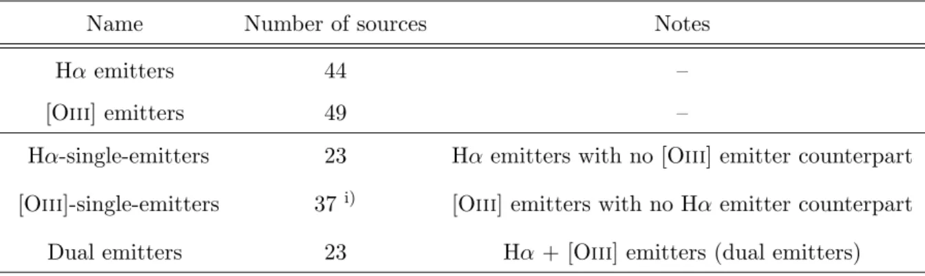
The HiZELS NB survey in the COSMOS field covers a very wide area of 1.6 deg², but the survey depth is different among the WFCAM pointings and among different NB filters (see Sobral et al. 2013). In this study, in order to ensure the same flux limit for both NB-selected samples, we use the sources in the deepest pointings only. The minimum exposure times are 107 ks and 62.5 ks for NBH and NBK, respectively. The survey area is then limited to the central ∼ 0.2 deg². The 3σ limiting fluxes for NBH and NBK are 3.60 × 10⁻¹⁷ erg s⁻¹cm⁻² and 2.96 × 10⁻¹⁷ erg s⁻¹cm⁻², respectively. In this study, we apply the same flux limit of 3.6 × 10⁻¹⁷ erg s⁻¹cm⁻² ([Oiii] flux for NBH and Hα+[Nii] flux for NB_K). As a result, 49 [Oiii] emitters and 44 Hα emitters remain in our final samples.

In Section 3.2.3, we focus on the galaxies detected with both [Oiii] and Hα emission lines (hereafter, dual emitters). When we search for the counterpart line, we lower the line detection threshold, as we can trust more the existence of a line at the expected wavelength in the other NB filter. We thus use the lower NBH (NBK) excess criteria, namely, EW ≳ 15 ˚A and/or Σ ≳ 2. We find 23 dual emitters in total. Among them, ten sources satisfy the original NB excess criteria of both NBH and NBK, indicating that they have the strong [Oiii] and Hα emission lines. Eleven (two) sources are the Hα ([Oiii]) emitters with the relatively weak [Oiii] (Hα) emission lines. The number of sources in each sample used here is summarized in Table 3.2.

We note that the transmission curves of NBH and NBK filters are not completely matched (Figure 3.1). The wavelength coverages of the two filters are transformed to the redshift space for each line in Figure 3.1 and Table 3.1. It turns out that ∼10% of the NBH

redshift coverage ([Oiii]λ5007) is completely out of the NB_K redshift coverage (Hα). In terms of FWHM ranges of the two NB filters, 24% of the NBH coverage is out of the NBK

coverage in redshift space. This mismatch of the redshift coverage is not critical when we compare the Hα emitters and [Oiii] emitters in Section 3.2.2. On the other hand, when we consider the sample of galaxies detected only by the [Oiii] emission line, the impact of this difference could be larger. The redshift mismatch might cause the loss of Hα flux from the galaxies which actually have the strong enough Hα emission line, and thus the observed [Oiii]/Hα ratio would become different from the intrinsic ratio. In such a case, the Hα flux would seem much lower with respect to [Oiii], and in the extreme case, the