Consortium Standards and Patent Pooling

(1)

Consortium Standards and

Patent Pooling

Reiko Aoki

Hitotsubashi University

(2)

Overview

• Lessons from Standard Consortiums

–

Free Riding

–

Bargaining Failure

• Patent Pools and Innovation

–

Upstream and downstream

–

Upstream = technology in the patent pools

(3)

Evidence from Standard

Consortiums

• Members leaving

–

Rambus left JEDEC and now suing members

• Patent owner does not join the pool,licenses

independently and charges “high” royalty

–

Forgent sues firms over JPEG patents

• DVD consortium split into 3 patent pools

• 3G platform

–

5 standards

(4)

Why is a Pool Not Stable?

• Welfare is greater when there is one single

patent pool

–

Competition authorities supportive

• Source of instability

–

Free riding by non-members

–

Bargaining failure due to heterogeneous

(5)

Example

• Demand for license depends on total

royalty payment (licensing fee)

• Higher royalty means fewer demand for

licenses

• Q = 60 – r

• Q is number of licenses demanded

• r is total royalty payment

–

If all patentees in one pool , then r is pool’s rate

(6)

There are three firms, A, B and C

• Single licensor

–

All three firms form a pool

• Independent licensing

–

There are three licensor

• Firm C is an outsider

–

Only firms A and B form a pool

(7)

Each licensor (pool or firm) sets

royalty to maximize own revenue

• If there are 3 licensors

–

Firm A charges r

_A

–

Total royalty payment is r

_A

+r

_B

+ r

_C

–

Firm A’s revenue (60 - r

_A

- r

_B

- r

_C

) x r

_A

• If there is one licensor (pool)

–

Pool charges r

–

Total royalty payment is r

(8)

Incentives

• Raising royalty reduces number of

licenses

• A’s revenue hurt by B and C’s royalty rate

–

Better to have fewer rivals

• A does not take into account reduction of

B and C’s revenue

(9)

Optimal Royalty and Revenue

Regime

No. of

Licensors

Each

Licensor

Royalty

Total

Royalty

Each

Licensor

Revenue

One Patent

Pool

1

30

30 30X30=

900 Firm C is

Outsider

2

20 20 x 2=

40 20X20=

400 Independent

Licensing

3

15 15 x 3=

45

(10)

Optimal Royalty and Revenue

Regime

No. of

Licensors

Each

Licensor

Royalty

Total

Royalty

Each

Licensor

Revenue

One Patent

Pool

1

30

30 30X30=

900 Firm C is

Outsider

2

20 20 x 2=

40 20X20=

400 Independent

Licensing

3

15 15 x 3=

45

(11)

Each Firm’s Revenue

Regime

Each

Licensor

Revenue

Each Firm Revenue

One Patent

Pool

900 900/3 =

300 > 225

Firm C is

Outsider

400 400/2 = 200 pool member

400 outsider > 300

Independent

(12)

Each Firm’s Revenue

Regime

Each

Licensor

Revenue

Each Firm Revenue

One Patent

Pool

900 900/3 =

300 > 225

Firm C is

Outsider

400 400/2 = 200 pool member

400 outsider

>

300 Independent

(13)

Free Riding

• C is better off being an outsider than being

a member of a pool

• Incentive to free ride

–

Good to have all other firms in a single pool

–

Better not to join

• Agree to a pool in principle and not join

• Leave the pool after formation

(14)

Possible Solutions

• 400 + 200 + 200 < 900

• Pool members are better off having firm C

join the pool

–

Pay 400 to firm C

(15)

Bargaining Failure

• Forgent and Rambus are not

manufacturers

• Research only firms (R-firms) and

vertically integrated (V-firms) have

different incentive

–

V-firms both conduct research and

manufacture

(16)

Different Profit and Incentives

• R-firm

–

Profit ( ) is only licensing revenue

• V-firm

–

Profit ( )

= Licensing revenue + manufacturing profit

–

Manufacturing profit decreasing in royalty rate

–

Wants royalty lower than R-firm

R



V

(17)

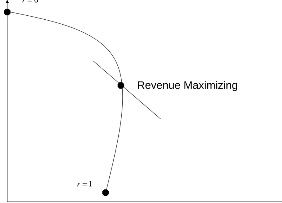
Patent Pool Licensing Frontier

• Plot of V-firm and R-firm profits with

different patent pool royalty rates (r)

• Pool revenue distributed according to

number of patents (in this example equal

number of patents)

(18)

V



R



Revenue Maximizing

0 

r

1 

r

(19)

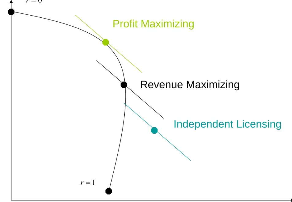
Possible Profit Allocations

• Revenue Maximizing Point = pool

revenue maximized

• Profit Maximizing Point

= total firm profits

maximized (r lower than Revenue Max)

• Independent Licensing Point

= Firms

(20)

V



R



Revenue Maximizing

Independent Licensing

Profit Maximizing

0 

r

1 

r

(21)

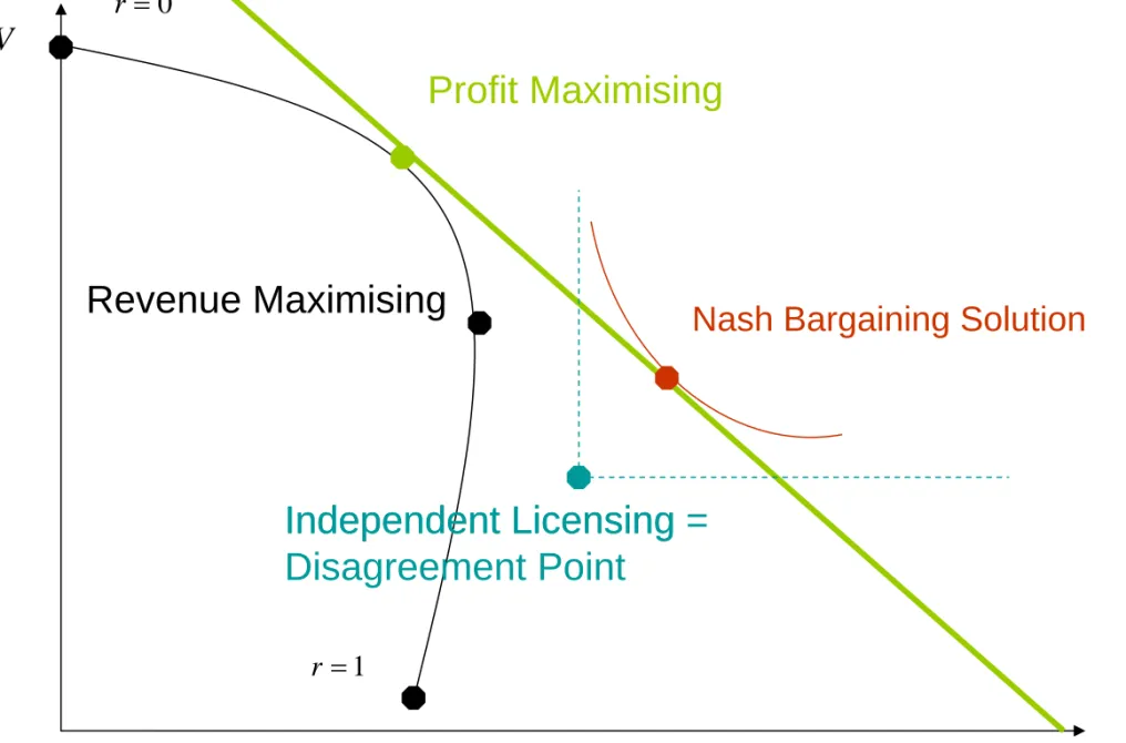
Bargaining Failure

• Independent Licensing is outside the

frontier

• Not achievable by current pool revenue

sharing rule

• Pool revenue sharing rule must

incorporate Independent Licensing into

account

(22)

Possible Solutions

• Total profit is larger with Revenue

Maximizing than Independent Licensing

• R-firm must be guaranteed at least

Independent Licensing profit

–

Bargaining than per patent distribution rule

• Total profit is larger even larger with Profit

Maximizing

(23)

Nash Bargaining Solution

• Profit maximizing line is bargaining frontier

–

Best possible profits by firms cooperating

–

Best achievable only by forming a pool

• Disagreement point (threat point) is

Independent Licensing

• Nash Bargaining Solution splits the

surplus from cooperating (difference

(24)

V



R



Independent Licensing

Profit Maximising

0 

r

1 

r

Figure 2: Nash Bargaining Solution

Nash Bargaining Solution

Revenue Maximising

(25)

Conclusion

• Patent pool is appealing in theory

• Problems in implementation (also

theoretically sound !)

–

Free riding

• Incentive to not join or leave the pool

• Wants everyone else to form a pool

–

Bargaining failure

(26)

Patent Pools and Innovation

◮ Problem:

◮ Downstream innovation or product development may

require licensing multiple upstream technologies with multiple owners⇒high transaction costs and ‘tragedy of the anticommons’.

◮ Example: Standard implementing patents, Genetic

diagnostic tests

◮ Possible solutions:

(27)

Patent Pools and Innovation

◮ Problem:

◮ Downstream innovation or product development may

require licensing multiple upstream technologies with multiple owners⇒high transaction costs and ‘tragedy of the anticommons’.

◮ Example: Standard implementing patents, Genetic

diagnostic tests

◮ Possible solutions:

◮ Patent Pools ◮ Cross-licensing ◮ Compulsory licensing ◮ Research exemptions

(28)

(29)

(30)

Focus

◮ Examine effects of PP onupstreamincentives to innovate

◮ PP of complementary intellectual property

◮ Standard implementing patent pools ◮ DNA microarrays

◮ Specifically, we examine how PPs effect

◮ Ex-post (after upstream innovation) licensing ◮ Ex-ante incentives to invest in upstream research.

◮ Compare different PP licensing revenue (royalty) distribution rules.

(31)

Focus

◮ Examine effects of PP onupstreamincentives to innovate ◮ PP of complementary intellectual property

(32)

Focus

(33)

Focus

◮ Compare different PP licensing revenue (royalty)

distribution rules.

(34)

Analysis - Factors to Consider

◮ Licensing by the PP must be optimalex-post(after

upstream innovation) given the ex-post outcome of innovation (market structure)

◮ Maximize joint profit

◮ Induce IP owners to rationally join

◮ R&D incentive determined byex-ante expected profit

◮ Ex-ante expected profitdepends onex-post profitandR&D technology(probability distribution over outcomes)

◮ Ex-post optimal royalty distribution rule may not provide

right incentives ex-ante

◮ Expected profit depends onnumber of firmsinvesting

(ex-ante market structure)

◮ Firms differ: Some firms arecompetitors(substitute

(35)

Analysis - Factors to Consider

◮ R&D incentive determined byex-ante expected profit

◮ Ex-ante expected profitdepends onex-post profitandR&D technology(probability distribution over outcomes)

(36)

Analysis - Factors to Consider

◮ R&D incentive determined byex-ante expected profit ◮ Ex-ante expected profitdepends onex-post profitandR&D

technology(probability distribution over outcomes)

◮ Firms differ: Some firms arecompetitors(substitute

(37)

Main Conclusions

◮ In general, PPsstimulate upstream R&D investment

◮ But PPs mayhurtthe incentive of an inventor withunique

ability (ex-ante monopoly, firms ex-ante asymmetric)

◮ PP dilutes rent

◮ And incentives to invest may be socially excessive

◮ PP that distributes licensing revenueunequallyamong its

members isless likelyto lead to welfareloss

◮ Unequal distribution helps form PP

◮ Even if inventors are symmetric ex-ante, ex-post

asymmetries may emerge

(38)

Main Conclusions

◮ PP dilutes rent

◮ Firm’s profit ranking over different PP rules differsex-ante or ex-postandby firm(monopolist or not)⇒likely to lead todisagreementover PP rules and formation

◮ Implication: Determination ofPP rules(revenue

(39)

Main Conclusions

◮ PP dilutes rent

◮ Firm’s profit ranking over different PP rules differsex-ante

(40)

Main Conclusions

◮ PP dilutes rent

◮ Firm’s profit ranking over different PP rules differsex-ante

or ex-postandby firm(monopolist or not)⇒likely to lead todisagreementover PP rules and formation

◮ Implication: Determination ofPP rules(revenue

(41)

Framework

◮ Newdownstream productneeds two complementary

upstream innovations: A and B.

◮ Large number of competitiveupstream research firms:

◮ Each has capacity for one research‘project’at costc ◮ Specialized in development of A or B

◮ Revenues only from licensing

◮ Eachfirmeither independently succeeds or fails

(probabilistic) .

◮ All successful projects (= patent) of a single component

result in perfect substitutes.

◮ PP

(42)

Framework

(probabilistic) .

◮ PP

◮ Licenses on behalf of successful inventors who choose to

join.

◮ Objective is to maximize joint royalty revenues of its

(43)

Framework

(probabilistic) .

◮ PP

(44)

Timing

◮ Innovation and licensing takes place in four stages:

I. Theantitrust ruleis set and announced: Is the PP allowed to jointly license substitute innovations or not?

II. The PP sets and announces aroyalty redistribution rule

consistent with the anti-trust rule.

III. Each research firmdecides to invest or not to investin an R&D project and those that invest invent a component with given probability.

(45)

Timing

II. The PP sets and announces aroyalty redistribution rule

consistent with the anti-trust rule.

(46)

Timing

II. The PP sets and announces aroyalty redistribution rule consistent with the anti-trust rule.

(47)

Timing

(48)

Timing

(49)

(50)

Assumptions

◮ Tragedy of Anticommons:

πM ≥2πDandW0≥WM ≥WD.

◮ π_M andW_M: Monopoly licensing profit and welfare. ◮ π_DandW_D: Duopoly licensing profit and welfare. ◮ W

0: Welfare when both components are licensed at zero

price

◮ P(k,N):Probabilitythatk substitute versions of a

component are invented whenN _{projects are undertaken}

for that component (probability ofk _{success from}N_trials):

N

X

k₌0

P₍k_,N_{) =}₁andlim_N→∞P(k,N) =0.

(51)

Assumptions

◮ Tragedy of Anticommons:

πM ≥2πDandW0≥WM ≥WD.

◮ π_M andW_M: Monopoly licensing profit and welfare. ◮ π_DandW_D: Duopoly licensing profit and welfare. ◮ W

0: Welfare when both components are licensed at zero

price

◮ P(k,N):Probabilitythatk substitute versions of a

component are invented whenN _{projects are undertaken}

for that component (probability ofk _{success from}N_trials):

N

(52)

Licensing Revenue and Antitrust Rules

◮ (π=total PP licensing revenues)

◮ Joint licensing of substitutes isnotallowed:

◮ Strict Antitrust Rule: PP randomly chooses at most one

member of each component to license; royalties are shared equally between the chosen.

◮ Joint licensing of substitutes by the PP is allowed:

◮ Equal:Withnmembers, each receivesπ/n.

◮ Unequal: If one component has a single inventor and the

other component hasn≥2 substitute inventors, the single

inventor receivesz_πand the others receive(1−z_)π/nwith

z ∈[0,1]. Otherwise, equal shares.

(53)

(54)

Ex-post Outcomes and PP Membership

◮ Possible ex-post outcomes: n_A andn_B(number of successful _{inventors of A and B) :}

Cases\Successful firms nA nB

Case MM 1 1

Case MC: 1 ( 2 or more) 2 or more (1)

Case CC: 2 or more 2 or more

◮ Who will join the PP ex-post?

◮ Competitive component inventors (cases MC & CC) join

any kind of PP.

◮ Competition among perfect substitutes drives royalties down

to zero⇒joining is a weakly dominant strategy for them.

◮ Case MM:Both inventors join any kind of PP. ◮ _{Avoid tragedy of anticommons .}

◮ Case MC: Monopoly inventor joins a strict PP. (Assumption)

Monopoly inventor doesnot joinan equal PP butdoes join

(55)

Ex-post Outcomes and PP Membership

Case MM 1 1

any kind of PP.

(56)

Ex-post Outcomes and PP Membership

Case MM 1 1

any kind of PP.

◮ Case MM:Both inventors join any kind of PP. ◮ _{Avoid tragedy of anticommons .}

◮ Case MC: Monopoly inventor joins a strict PP.(Assumption)

Monopoly inventor doesnot joinan equal PP butdoes join

(57)

Ex-post Outcomes and PP Membership

Case MM 1 1

any kind of PP.

(58)

Ex-post Profits

◮ Ex-post equilibrium payoffs of successful inventors

(Gains,Lossesrelative to no PP):

PP Type\Profit πMM πMCM π C

MC(n) πCC(nA,nB)

None πD πM 0 0

Equal πM/2 πD πD/n πM/(nA+nB)

Unequal πM/2 zπM (1−z)πM/n πM/(nA+nB)

Strict πM/2 πM/2 1_nπM/2 _n1

iπM/2;

(59)

Ex-post Welfare

◮ Ex-post equilibrium welfare:

(Gains,Losses)

PP Type\Welfare W_MM W_MC W_CC

None W_D W_M W₀

Equal W_M W_D W_M

Unequal W_M W_M W_M

Strict W_M W_M W_M

◮ Ex-ante only probability of outcomes (MM,MC, orCC)

(60)

(61)

R&D Technology

◮ Probability that a given research firm becomes a

successful inventor depends on the number of firms that invest.

(62)

Upstream Innovation

◮ Ex-ante expected profit depends on ex-post profit and

distribution of outcomes

◮ We consider two different upstream market structures.

◮ Market 1: There areN _≥2 firms that can invest in A and N ≥2 firmsthat can invest in B.

◮ Potential ex-ante competition for both components. ◮ Symmetric

◮ Market 2: There isonly one firmthat invests in A.N _≥2 firmscan invest in B.

◮ Ex-ante monopoly for innovation of component A.

Competitive for component B.

(63)

Upstream Innovation

◮ Ex-ante expected profit depends on ex-post profit and

distribution of outcomes

◮ We consider two different upstream market structures. ◮ Market 1: There areN _≥2 firms that can invest in A and

N ≥2 firmsthat can invest in B.

◮ Potential ex-ante competition for both components. ◮ Symmetric

◮ Market 2: There isonly one firmthat invests in A.N _≥2

firmscan invest in B.

◮ Ex-ante monopoly for innovation of component A.

(64)

Market 1 Upstream Innovation

◮ Market 1:Nprojects are undertaken for each component ◮ Ex-ante competitive, symmetric

◮ Ex-ante expected profit and welfare:

π(N_{) =} 1

NP(1,N)

2

πMM

+_N1P₍_1,N₎

N

X

k₌2

P₍k_,N₎h_πM_MC₊n_πC

MC(k)

i

+

N

X

m₌2

N

X

k₌2

m

NP(m,N)P(k,N)πCC(m,k)−c

W ₍N_{) =} P₍_1,N₎2W_MM₊₂P₍_1,N₎

N

X

k₌2

P₍k_,N₎W_MC

+ N X m 2 N X k 2

(65)

Market 1 Result: Ex-ante Expected Profit and Welfare

(Given

N

₎

◮ Ex-ante, theexpected profit gains always outweigh any

losses:

◮ πUC(N) =πSC(N)_≥πEC(N)_≥πNC(N)for allN _≥1.

◮ PP increases incentive to invest in upstream R&D.

◮ Welfare

◮ WhenNis large, case CC likely andW

0achieved. ◮ WhenNis small, case MM likely and PP beneficial.

◮ Expected welfare withno PPis highest whenNis large but lowest whenN _{is small:}

(i) WUC

(N_{) =}WSC

(N₎≥WEC

(N₎≥WNC

(N₎for smallN,

(ii) WNC

(N₎≥WUC

(N_{) =}WSC

(N₎≥WEC

(66)

Market 1 Result: Ex-ante Expected Profit and Welfare

(Given

N

₎

losses:

◮ PP increases incentive to invest in upstream R&D. ◮ Welfare

0achieved.

◮ WhenNis small, case MM likely and PP beneficial.

◮ Expected welfare withno PPis highest whenNis large

but lowest whenN _{is small:}

(i) WUC

(N_{) =}WSC

(N₎≥WEC

(N₎≥WNC

(N₎for smallN,

(ii) WNC

(N₎≥WUC

(N_{) =}WSC

(N₎≥WEC

(N₎for largeN. ◮ _{Unequal or strict PP always outperforms equal: Unequal or strict}

(67)

Market 1 Result: Ex-ante Expected Profit and Welfare

(Given

N

₎

losses:

◮ PP increases incentive to invest in upstream R&D. ◮ Welfare

0achieved.

◮ WhenNis small, case MM likely and PP beneficial.

◮ Expected welfare withno PPis highest whenNis large

but lowest whenN _{is small:}

(i) WUC

(N_{) =}WSC

(N₎≥WEC

(N₎≥WNC

(N₎for smallN,

(ii) WNC

(N₎≥WUC

(N_{) =}WSC

(N₎≥WEC

(68)

Simulation with Binomial Upstream R&D Technology

(Determination of

N

₎

◮ Linear demand for licenses:Q=100₋ρgives parameter

values:

Parameter πM πD W0 WM WD

Value 100₄ 100₉ 50 75₂ 250₉

◮ AssumeP(k,N)is binomial;σis success prob. of each

project.

◮ Other parameters:z,c (market 1),c_A andc_B(market 2).

◮ Given parameter values, use numerical search to find

equilibrium value ofN_{under each PP type.}

◮ Equilibrium condition: HighestNwhereπ(N)_≥0 and

(69)

Simulation with Binomial Upstream R&D Technology

(Determination of

N

₎

◮ Linear demand for licenses:Q=100₋ρgives parameter

values:

Parameter πM πD W0 WM WD

Value 100₄ 100₉ 50 75₂ 250₉

◮ AssumeP(k,N)is binomial;σis success prob. of each

project.

◮ Other parameters:z,c (market 1),c_A andc_B(market 2). ◮ Given parameter values, use numerical search to find

equilibrium value ofN_{under each PP type.}

(70)

Market 1 Ex-ante Profit & Welfare and Equilibrium

Investment by Simulation

◮ Simulation forc =2.5 andσ =0.7 (symmetry makes value

ofz _irrelevant):

◮ PP stimulates investment but may reduce welfare.

◮ Equilibrium investment may increase too much once R&D

(71)

Market 2 of Upstream Innovation

◮ Market 2: Firm A has theunique abilityto develop

component A ; Development of component B is as before

◮ Asymmetric firms, Firm A is a monopolist ◮ Case CC is no longer possible.

◮ Firm profits whenNprojects undertaken for component B:

πA(N) =P(1,N)πMM+ N

X

k₌2

P₍k_,N₎_πM_MC−c_A

πB(N) = 1

NP(1,N)πMM +

N

X n

NP(k,N)π

C

(72)

Market 2 of Upstream Innovation

◮ Market 2: Firm A has theunique abilityto develop

component A ; Development of component B is as before

◮ Asymmetric firms, Firm A is a monopolist ◮ Case CC is no longer possible.

◮ Firm profits whenNprojects undertaken for component B:

πA(N) =P(1,N)πMM+ N

X

k₌2

P₍k_,N₎_πM_MC−c_A

πB(N) =

1

NP(1,N)πMM +

N

X

k₌2 n

NP(k,N)π

C

(73)

Market 2 Results: Ex-ante Expected Profits and

Welfare (Given

N

₎

◮ Firm A prefers

◮ No PPwhenNis large ◮ Unequal PP whenNis small.

◮ Component B firm , for any givenN,

◮ Always better off under either an equal or unequal PP

compared to no PP.

◮ Such a firm is better off under an unequal PP compared to

an equal PP ifz ≤1−πD/πM.

◮ Welfare: Unequal or strict PP best for allN. Equal PP

(74)

Market 2 Results: Ex-ante Expected Profits and

Welfare (Given

N

₎

◮ Firm A prefers

◮ No PPwhenNis large ◮ Unequal PP whenNis small.

◮ Component B firm , for any givenN,

◮ Always better off under either an equal or unequal PP

compared to no PP.

◮ Such a firm is better off under an unequal PP compared to

an equal PP ifz ≤1−πD/πM.

◮ Welfare: Unequal or strict PP best for allN. Equal PP

(75)

Market 2 Upstream R&D Incentives

◮ PP’s effect depends on firm(ex-ante market structure)

◮ Increasethe incentives ofcompetitiveresearch firms to

invest, but

◮ Mayreducethe incentive ofmonopolist(unique ability).

◮ PP’s effect differ by firm andby ex-ante and ex-post.

◮ Ex-post, firm A prefers ahigh value ofzunder an unequal

PP, but this reduces the payoff of component B firms.

◮ Ex-ante, firm A may want to choose alower value ofzto

give incentive to B firms to invest.

(76)

Market 2 Upstream R&D Incentives

◮ PP’s effect depends on firm(ex-ante market structure)

◮ Increasethe incentives ofcompetitiveresearch firms to

invest, but

◮ Mayreducethe incentive ofmonopolist(unique ability).

◮ PP’s effect differ by firm andby ex-ante and ex-post.

◮ Ex-post, firm A prefers ahigh value ofzunder an unequal

PP, but this reduces the payoff of component B firms.

◮ Ex-ante, firm A may want to choose alower value ofzto

give incentive to B firms to invest.

◮ Or,ex-ante, firm A may prefernot to have a strict anti-trust

(77)

Market 2: Ex-ante Profit & Welfare and Equilibrium

Investment

◮ Single simulation of market 2, forc_A=8,c_B =1.3,σ =0.5

(78)

Interaction between Technology and Distribution Rule

by Simulation

◮ Effect of changingz in an unequal PP on equilibrium

expected profits of firm A and expected welfare:

◮ Level ofz affects equilibrium investment level of

component B firms.

(79)

Conclusion

◮ PP can generate both ex-post and ex-antegains and

lossesto welfare and profits of research firms.

◮ PP generallystimulate investmentin upstream R&D except

possibly by inventors who have unique abilities.

◮ Unequal PPredistribution is less likely to lead to welfare

losses but not always.

◮ Likely conflict between existing and potential inventors

regarding PP support.

◮ PP design and royalty distribution rule needs to reflect

(80)

Conclusion

◮ PP can generate both ex-post and ex-antegains and

lossesto welfare and profits of research firms.

◮ PP generallystimulate investmentin upstream R&D except

possibly by inventors who have unique abilities.

◮ Unequal PPredistribution is less likely to lead to welfare

losses but not always.

◮ Likely conflict between existing and potential inventors

regarding PP support.

◮ PP design and royalty distribution rule needs to reflect

(81)

References (1)

• R. Aoki and S. Nagaoka, “The Consortium

Standard and Patent Pools”, The Economic

Review, 55(4):346-356, 2004.

• R. Aoki and S. Nagaoka, “Coalition Formation

for a Consortium Standard Through a Standard

Body and a Patent Pool: Theory and Evidence

from MPEG2, DVD and 3G”, Institute of

Innovation Research Working Paper WP#05-01,

2005

.

(82)