A Study on the Photospheric Polar
Magnetic Patches of the Sun as
Revealed with Hinode
A dissertation submitted in partial fulfillment of
the requirements for the degree of
Doctor of Philosophy
by
Anjali John Kaithakkal
Department of Astronomical Science,
School of Physical Science,
The Graduate University for Advanced Studies
First of all, I would like to thank my advisors, Associate Professor Yoshinori Suematsu, Assistant Professor Masahito Kubo and Professor Tetsuya Watanabe for their invaluable guidance and support. My special thanks to Professor Saku Tsuneta for inspiring discussions and guidance. My sincere thanks to Dr. Daikou Shiota for helping me out with IDL programming and data analysis. I also like to thank Dr. Yusuke Iida for providing me his code to use for my study.
I would like to thank Dr. Ryohko Ishikawa who was always ready to help me out with science and everyday life in Japan. My thanks to Drs. Robert Cameron, D. Orozco Suarez, Yukio Katsukawa, Takashi Sakurai, Toshifumi Shimizu, Takashi Sekii and Kiyoshi Ichimoto for useful discussions. I thank (soon to be Dr.) Nobuharu Sako and other members of the solar physics group of National As- tronomical Observatory for making my stay in Japan comfortable.
Data for my study were taken from spectropolarimeter (SP) of Solar Optical Telescope (SOT) aboard Hinode satellite. Hinode is a Japanese mission developed and launched by ISAS/JAXA, collaborating with NAOJ as a domestic partner, NASA and STFC (UK) as international partners. Scientific operation of the Hin- ode mission is conducted by the Hinode science team organized at ISAS/JAXA. This team mainly consists of scientists from institutes in the partner countries. Support for the post-launch operation is provided by JAXA and NAOJ (Japan), STFC (UK), NASA, ESA, and NSC (Norway).
i
I would like to thank the Ministry of Education, Culture, Sports, Science, and Technology (MEXT) of Japan for financial support through its doctoral fellowship program for foreign students and the Graduate University for Advanced Studies (GUAS / SOKENDAI) for an associate researchers grant.
Last but not least, I am deeply grateful to my parents and siblings for their prayers, constant support and encouragement. I am very thankful that God had blessed me with such amazing people in my life.
ii
The distribution and evolution of the Sun′s polar magnetic field is of vital im- portance to understand the origin of the solar magnetism, its periodic variation and the heliospheric magnetic flux. Recent high resolution observations from the Hinode satellite have revealed that the polar region is dominated by unipolar mag- netic patches which possess magnetic fields with field strengths exceeding 1 kG. The basic properties, mechanism of formation and reversal of the polar magnetic fields are topics which are yet to be resolved. Our purpose is to quantitatively study the spatial fine structure of and interaction of photospheric plasma flows with the polar magnetic patches using observations obtained with the Solar Op- tical Telescope (SOT) aboard the Hinode satellite. The advantage with Hinode is that, it provides unprecedented observations with high polarimetric sensitivity and spatial resolution even at higher solar latitudes.
We carried out a statistical study of the relation between polar magnetic patches and polar faculae. Polar faculae are unique because they take part in the activity cycle and their count is considered as a good proxy for the polar magnetic field. They are bright, small-scale magnetic features observed at higher heliographic latitudes. Previous studies have shown that polar faculae cycle has a periodicity of 11- years and is out-of-phase with the sunspot cycle. To obtain the correlation between polar faculae and the polar magnetic patches, we used observa- tions of the north polar region taken in 2007 September for our study. The period of observation is close to the solar cycle minimum, and hence the polar faculae
iii
occurrence is maximum. We found that polar faculae are enclosed within majority of the magnetic patches with flux greater than 1018Mx. Magnetic patches without polar faculae dominate in the flux range below 1018 Mx. The faculae are consider- ably smaller than their parent patches, and single magnetic patches contain single or multiple faculae. The faculae in general have higher intrinsic magnetic field strengths than the surrounding regions. We found that faculae flux alone cannot account for the magnetic flux from the polar region.
We investigated the role of photospheric flow fields in the formation and evo- lution of the polar magnetic patches. To obtain this we used a time series of maps of vector magnetic fields obtained with SP. We observed unipolar appearance and disappearance in the data. Converging horizontal flows are observed outside of the magnetic patches during the entire life time of the patches. The converging flow is best observed at a height close to the solar photosphere. We also observed a weak converging flow around the retraced patch location 16 minutes before the patch appearance. We suggest that polar magnetic patches are formed by the accumu- lation of flux fragments by the horizontal converging flows. In addition to direct cancellation between opposite polarity patches we observed unipolar disappear- ance of polar patches. We speculate that these patches diffuse away into smaller fragments with flux below the detection limit of the instrument and eventually undergo cancellation with opposite polarity fragments.
To understand the various mechanisms involved in the reversal of the polar magnetic field and the dynamic activities caused by the interaction between flows and magnetic field, continuous observations with high spatio-temporal resolution are necessary.
iv
1 Introduction 3
1.1 The Polar Magnetic Field . . . 3
1.2 Purpose of the Thesis . . . 10
2 Association between Polar Faculae and Polar Magnetic Patches 13 2.1 Introduction . . . 13
2.2 Observations. . . 14
2.2.1 Identification of Polar Facular Pixels within Magnetic Patches 17 2.3 Results . . . 22
2.3.1 Majority Polarity Patches . . . 23
2.3.2 Minority Polarity Patches . . . 26
2.4 Discussion . . . 26
3 Photospheric Flow Field Related to the Evolution of Polar Mag- netic Patches 33 3.1 Introduction . . . 33
3.2 Observations. . . 35
3.2.1 Identification and Tracking of Magnetic Patches . . . 39 v
1
3.3 Results . . . 40 3.3.1 Lifetime and Magnetic Flux Distribution of the Samples . . 40 3.3.2 Appearance of Faculae within Magnetic Patches . . . 43 3.3.3 Flow Field at the Time of Appearance and Disappearance
of Magnetic Patches . . . 45 3.4 Summary and Discussion . . . 65
4 Concluding Remarks 75
4.1 Summary . . . 75 4.2 Future Work . . . 78
Chapter 1
Introduction
1.1 The Polar Magnetic Field
The diverse and dynamic phenomena occurring on the Sun is a consequence of interaction between solar plasma and the Sun′s magnetic field. The magnetic ac- tivity of the Sun is characterized by its cyclic variation with a period of 22 years. According to current understanding, the Sun′s magnetic field is produced and maintained by a solar dynamo (Babcock 1961; Leighton 1969; Charbonneau 2010). The Sun′s large-scale magnetic field is decomposed into toroidal and poloidal com- ponents. The dynamo mechanism involves recycling of these two components. The intense toroidal flux tubes, produced by the differential rotation acting upon the poloidal field emerge buoyantly through the solar convection zone and manifest on the surface as tilted bipolar sunspot pairs. The sunspots eventually decay and the remnant magnetic flux, dominant contribution to which comes from the trail- ing sunspots, is then transported to the polar region to regenerate the poloidal magnetic component (Babcock 1961; Leighton 1969).
3
The polar magnetic fields attain maximum strength during solar cycle mini- mum (corresponds to a period of minimum sunspot number) and become weak near the solar cycle maximum. One of the remarkable aspects of the polar mag- netic field is its reversal around the maxima of 11-year sunspot cycles. Reversal of the polar magnetic fields was first reported by Babcock (1959). The 22-year magnetic cycle and the reversal of the polar magnetic field near the maximum of the solar cycle can be seen in Fig.1.1. Standard surface flux transport models interpret that the reversal of the polar magnetic fields is an outcome of magnetic flux transported to the polar caps from the active latitudes, by supergranular dif- fusion and meridional circulation (Babcock 1961; Leighton 1964; Wang et al. 1989; Sheeley 2005).
Reversal of the polar magnetic fields do not take place simultaneously in the north and south polar regions (Babcock 1959; Makarov & Sivaraman 1986; Shiota et al. 2012; Svalgaard & Kamide 2013). Rightmire-Upton et al. (2012) pointed out that the asymmetric polar field reversal may arise from the asymmetry in the meridional flow velocities. Some other studies suggest that the asymmetry in the polar field reversal is associated with asymmetric solar activity cycle in the respective hemispheres (Svalgaard & Kamide 2013; Mordvinov & Yazev 2014). The polar field reversal is reported to depend also on variation of the tilt angle of bipolar sunspots with latitude (Zolotova & Ponyavin 2013). They showed that an increase in the tilt angle of the spots with latitude is essential to reproduce the observed polar field reversal. The reversal is not an instantaneous process and in some solar cycles the polar region was observed to undergo two- or three-fold temporary reversals before the reversal is completed (e.g. Makarov & Sivaraman 1989; Benevolenskaya 1996).
1.1. THE POLAR MAGNETIC FIELD 5
Figure 1.1: Magnetic butterfly diagram. The figure depict the radial component of the solar surface magnetic field. Reproduced from http://solarscience.msfc. nasa.gov/dynamo.shtml, which was prepared by D.Hathaway.
There are some distinct phenomena which mark the reversal of the polar mag- netic fields. The rapid migration (”rush to the poles”) of polar crown filaments (Hyder 1965, Makarov, Tlatov, & Sivaraman 2001), the disappearance of polar coronal holes (Waldmeier 1981, Harvey & Recely 2002) and cessation of high- latitude coronal mass ejections (CMEs)(Gopalswamy et al. 2003) indicate the onset of the polar field reversal. However, the mechanism that drives the polar field reversal is still an open issue and the prediction of the exact timing of the reversal is still difficult. Surface flux transport models suggest that the polar field reversal is realized by cancellation of the existing polar flux by the decayed active region flux of opposite polarity advected to the polar caps. Fisk & Schwadron (2001) argues that the reversal of polar magnetic fields is an outcome of the diffu- sive motions of the open magnetic field lines on the solar surface caused by their
reconnection with the randomly oriented closed loops. They also suggest that the reversal is a surface effect. Gopalswamy et al. (2003) proposed that the CMEs could be one of the possible mechanisms by which the open magnetic fields in the polar region decay during the reversal process.
The polar magnetic field and its reversal are of vital importance in understand- ing the origin of the solar magnetism and its periodic variation. Strength of the polar magnetic field in one solar cycle is employed to predict the strength of the successive solar cycle (Schatten et al. 1978; Choudhuri et al. 2007). The polar magnetic field is also considered as the origin of the fast polar solar wind. De- spite the great importance of solar polar areas to understand numerous solar and astrophysical phenomena like the solar activity cycle, coronal heating, solar wind acceleration, etc., the polar regions are not yet sufficiently studied. The accurate measurement of polar magnetic fields is greatly limited by the foreshortening of the solar surface magnetic structures near the limb as well as instrumental limitations in terms of sensitivity and accuracy .
The previous studies on the polar magnetic fields were mainly based on line of sight (LOS) magnetograms. The observed magnetic fields are interpreted as the LOS component of the radial field and is corrected for by dividing by the cosine of the heliocentric angle (e.g., Svalgaard et al. 1978, Wang et al. 1989). Varsik et al. (1999) reported, using LOS magnetograms, that the polar caps are occu- pied by large unipolar regions which enclose magnetic knots of opposite polarities and that within a given unipolar region knots of one polarity dominate the other during cycle minimum. Using chromospheric LOS magnetograms Raouafi et al. (2007) speculated the possible existence of two kinds of magnetic concentrations in the polar regions: small flux elements which are uniformly distributed in the
1.1. THE POLAR MAGNETIC FIELD 7
polar caps, with a probable local origin and large flux elements originating from the decayed active region flux. The issues with the LOS magnetograms are; 1) the LOS component of the radial field does not produce large signals and hence the resulting field measurements will be weak, and 2) it is mixed with dynamic horizontal components (Harvey et al. 2007), which when corrected for projection effects might enhance noise signals.
To follow the distribution and cyclic variation of polar magnetic flux, proxies were and are still being used. Polar faculae, observed in the higher solar latitudes, are one such proxy. They are bright and are associated with magnetic fields. Polar faculae exhibit a periodic variation which is out of phase with the solar cycle (Saito & Tanaka 1960, Makarov & Makarova 1996, Deng et al. 2011). The cyclic variation of sunspot number and polar faculae count are shown in Fig.1.2. The count of polar faculae is considered as good proxy for the polar magnetic flux.
Faculae observed at lower heliographic latitudes near the limb are referred to as′′active region (AR) faculae′′. They are seen particularly around sunspot active regions. Excess brightness of both AR and polar faculae in comparison with the quiet sun continuum intensity is explained based on the ”hot wall effect” (Spruit 1976, Keller et al., 2004). Faculae are generally described as magnetic features with vertically oriented evacuated flux tubes. As a result of evacuation, flux tubes appear transparent. When observed at an inclined angle the hot wall of the flux tubes is visible causing the flux tubes to appear bright (”hot wall effect”) in the continuum intensity images. Another important aspect that make the study of faculae, whether AR or polar, an interesting research topic is its contribution to the variations in total solar irradiance (e.g., Foukal et al. 2004).
The advantage with Hinode (Kosugi et al. 2007) is that it enabled unprece-
Figure 1.2: The smoothed monthly sunspot numbers (solid black line) and polar faculae (bold solid black line), in the northern hemisphere (a) and southern hemi- sphere (b), respectively. The vertical solid and dashed lines represent the minimum and maximum of each solar cycle, respectively (Deng et al. 2011). Polar faculae data were taken from National Astronomical Observatory of Japan (NAOJ) and sunspot data from Temmer et al. (2006).
1.1. THE POLAR MAGNETIC FIELD 9
dented observations of the polar regions with high spatial resolution and polarimet- ric (magnetic) sensitiveity and provides vector magnetic field information. Recent high-resolution observations with the spectropolarimeter (SP; Lites et al. 2013) of the Solar Optical Telescope (Ichimoto et al. 2008; Shimizu et al. 2008; Suematsu et al. 2008; Tsuneta et al. 2008b) aboard Hinode have shown that the polar region is dominated by unipolar magnetic patches of concentrated magnetic fields oriented vertical to the local surface with strengths exceeding 1kG (Tsuneta et al. 2008a; Ito et al. 2010). Tsuneta et al. (2008a) reported that the kilogauss patches exhibit spatial coincidence with polar faculae. Using observational data taken dur- ing the period of solar cycle minimum, Ito et al. (2010) found that the average area and the total magnetic flux of the polar patches are larger than those of the quiet Sun region in the lower latitudes. They also observed that the vertical flux distribution is balanced in the low-latitude quite Sun, whereas it is asymmetric in the polar region; The vertical flux distribution with the polarity same as that of the polar magnetic field dominates over the other polarity. They also found that total magnetic flux of the polar region is larger than that of the quiet Sun. Shiota et al. (2012) reported that the magnetic patches in the polar region are classified into two categories: the small-flux concentrations (<1018Mx), which are of mixed polarity with balanced fluxes, and the large-flux patches (≥1018 Mx) scattered over the polar region, which are unipolar. The authors also found that large-flux patches are modulated by the solar cycle.
1.2 Purpose of the Thesis
The Sun’s polar magnetic field plays an active role in manifesting many of the observed dynamic phenomena in the Sun. To throw light into these solar phenom- ena it is crucial to comprehend the evolution and properties of the polar magnetic fields in both global and local scale. Erstwhile studies focused mainly on the cyclic variation of polar magnetic flux rather than on their local scale distribution and evolution. As polar magnetic flux is concentrated in the form of patchy structures, it is the aggregate of this individual patches that contribute to the global scale behavior of the polar magnetic flux over the course of solar cycles. The main focus of this thesis is to understand the properties of individual polar magnetic patches and the role of photospheric plasma flows in the formation and evolution of such patches.
High resolution spectropolarimetric observations provided by Hinode has made the direct determination of magnetic flux of individual polar patches possible. However, the fine structure and properties of individual polar patches in terms of distribution of magnetic parameters and intensity are yet to be investigated. Further, the relation between polar magnetic patches and polar faculae, which are used as proxy while studying the cyclic variation of polar magnetic flux, is also unknown. Comprehension of this relationship is essential to understand the contribution of polar faculae to the polar flux. Though polar flux is believed to be originated from surplus magnetic flux of the decayed active regions, it still remains unexplored as to how: a) magnetic flux in the polar region is concentrated in the form of unipolar magnetic patches, and b) these magnetic patches decay and eventually reverse the polarity of the polar field.
1.2. PURPOSE OF THE THESIS 11
Chapter 2 describes statistical study of: a) the association between polar mag- netic patches and polar faculae, and b) the properties of the magnetic patches like magnetic field and its local zenith angle, intensity, etc using observations from Hinode SOT/SP of the north polar region. Chapter 3 mainly delineates the in- fluence of photospheric surface flows in the evolution of polar magnetic patches. SP observations of the north and south polar region, with 16 min cadence and 6 hr duration, are used for this study. Finally, summary of the thesis is outlined in Chapter 4.
Chapter 2
Association between Polar
Faculae and Polar Magnetic
Patches
2.1 Introduction
Polar faculae are bright, small-scale structures visible in white light and in chromospheric lines. They populate higher heliographic latitudes, above 60◦ (e.g.,Okunev & Kneer 2004; Blanco Rodr´ıguez et al. 2007) or 70◦(Mu˜noz-Jaramillo et al. 2012). Okunev & Kneer (2004) found that the contrast of polar faculae de- creases monotonically toward the extreme limb, whereas Blanco Rodr´ıguez et al. (2007) reported that the contrast remains constant or may even increase toward the limb.
The number of polar faculae is considered to be a good proxy for the polar magnetic flux. It follows an 11 yr cycle that is out-of-phase with the sunspot
13
cycle (Makarov & Makarova 1996; Sheeley 2008; Mu˜noz-Jaramillo et al. 2012). The faculae become visible after the reversal of the polar magnetic field around sunspot maximum, and their numbers reach a maximum at sunspot minimum. Homann et al. (1997) and Okunev & Kneer (2004) found that polar faculae have magnetic field strengths in the kilogauss range and that they are unipolar, with the same polarity as the observed global polar field. However, Blanco Rodr´ıguez et al. (2007) reported the existence of faculae having polarities opposite to that of the polar field.
Tsuneta et al. (2008a) reported that the kilogauss patches coincide in position with polar faculae, but the true nature of the relationship between polar faculae and the polar magnetic patches remains elusive. In this paper, we investigate how closely the faculae are associated with the magnetic patches by studying their polarity and intrinsic field strength, the inclination of the magnetic field vector with respect to the local normal (zenith angle), and their contribution to the magnetic flux of the observed polar region. We also attempt to determine parameters that control the brightness of polar faculae. These observations correspond to a phase of solar minimum and, hence, to a maximum of polar faculae. At the time of the observations, the polarity of the north polar cap was negative. We hereafter refer to magnetic patches with negative polarity as majority (dominant) polarity patches and those with positive polarity as minority polarity patches.
2.2 Observations
Information about the north polar region observations carried out by the Hinode SOT/SP in 2007 September is given in Table 2.1. Each map of the polar region
2.2. OBSERVATIONS 15
was acquired through several hours of slit-scan observations. The SP provides the full Stokes I, Q, U , and V profiles of the Fe i 630.15 and 630.25 nm spectral lines, including the nearby continuum with a spectral sampling of 2.155 pm. The integration time for each slit position is 9.6 s. The scanning step is 0′′.15 and the spatial sampling along the slit is 0′′.16. The raw SOT/SP data were calibrated using the spprep routine (Lites and Ichimoto 2013), available in the SSW package to account for dark current, flat fielding, instrumental cross talk and orbital drift along the wavelength axis. The noise level estimated from the continuum in the Stokes V spectrum is 1.1×10⁻³Ic, where Ic is the continuum intensity.
The magnetic field parameters are deduced by using a least-squares fit to the Stokes profiles using the MILOS code (Milne-Eddington Inversion of Polarized Spectra; Orozco Su´arez & del Toro Iniesta 2007). MILOS assumes a two-component atmosphere model (magnetic and nonmagnetic) in a pixel. The inversion code pro- vides: three components describing the vector magnetic field - the field strength B, the inclination between the line-of-sight (LOS) and the field vector, and the azimuth of the field vector in a plane perpendicularar to the LOS, the LOS ve- locity, two parameters describing the linear source function, the ratio of line to continuum absorption coefficients, the Doppler width, the damping parameter, and the stray-light factor α. The stray-light factor, α quantifies contribution to the measured intensity from both a non-magnetic area of the pixel and stray light contamination arising from instrument optics. From the stray-light factor the mag- netic fill fraction - fraction of a pixel occupied by magnetic field - is calculated as f = 1 − α(Orozco Su´arez et al. 2007), provided the stray-light contamination is negligible. All these parameters are in the observer’s frame.
The inversion is performed only for pixels whose linear or circular polarization
signal amplitudes exceed a given threshold above the noise level which depends on the exposure time. The noise level σ′ is determined in the continuum wavelength range of the Stokes V profiles and is given by
q P
i(Vi− V )
2/n), where Vi is the intensity of the Stokes V profile at continuum wavelength pixel i, V is the average Stokes V signal for the same wavelength range, and n is the number of wavelength data points. The pixels with Stokes Q, U or V peak larger than 5 times the noise level alone are fitted using the code. Those pixels with the absolute value of the Doppler velocity higher than 10 km s−1 or the filling factor less than 0.01 are removed since it was found that the Stokes profiles of such pixels are not fitted well.
The azimuth value provided by the inversion is ambiguous by 180◦. This am- biguity in the transverse magnetic fields was resolved by employing the method of Ito et al. (2010): The vector magnetic field for each pixel will have two solutions for the local zenith angle as a result of the ambiguity. We assume that the mag- netic field vector is nearly vertical to the local solar surface and the ambiguity was resolved by selecting the value with the most vertical field in the local frame.The direction is deemed to be vertical if the zenith angle is between 0◦ and 40◦ or between 140◦ and 180◦.
For this study we consider only the vertical magnetic field as the magnetic field vectors associated with polar patches are nearly vertical to the local surface (e.g., Tsuneta et al. 2008a).The vertical magnetic flux is defined as PjBjfjcos ijAj, where Bj, fj, ij, and Aj are the intrinsic field strength, magnetic filling factor, local zenith angle, and pixel area, respectively, for the jth CCD pixel. The pixel area was corrected for projection effect. Since the magnetic field in the polar region is distributed as isolated patches, neighboring pixels with the same polarity are
2.2. OBSERVATIONS 17
grouped into patches following the method described by Shiota et al. (2012), and each is given a signed identification number based on its polarity.
2.2.1 Identification of Polar Facular Pixels within Mag-
netic Patches
Magnetic patches at heliographic latitudes above 70◦ with at least 4 pixels, cor- responding to the spatial resolution of the telescope, were selected for our study. Patches with µ (cosine of the heliocentric angle) less than 0.126, corresponding to a heliocentric angle of 82◦.8, were ignored, since the granular structure is not recoverable beyond this angle.
We picked up magnetic patches and then identified facular pixels inside each patch in the normalized continuum intensity maps. The continuum intensity (Ic) map is obtained by integrating the Stokes I profile outside the absorption lines. The integration ranges were 6300.98–6301.08 and 6302.90–6302.99 ˚A. A smoothed map representing the center-to-limb variation (CLV) of the continuum intensity, hIci, is obtained as follows: A least-squares surface fit using a 5th-order polynomial in µ (following Pierce et al. 1977) is performed on the Ic map. The fitted map is then subtracted from the original, and the standard deviation σ0 of the difference is calculated. We then remove the bright and dark features from the original image using a ±3σ0 cutoff, and a fit with same functional form is performed to obtain a CLV function unaffected by the presence of faculae. The normalized intensity is defined as Ic/hIci, where Ic and hIci are the continuum intensity and the intensity averaged over the same µ-value, respectively. An example of continuum intensity map and the corresponding normalized intensity map are shown in Figures 2.1 and
2.2 respectively.
Figure 2.3 shows the scatter plot of normalized intensity as a function of µ. The spikes in the plot are attributed to polar faculae, while smaller fluctuations about 1.0 are ascribed to granulation. Within each magnetic patch, pixels having intensity greater than or equal to a given threshold are classified as belonging to polar faculae. The threshold to identify facular pixels varies with µ. The standard deviation σ of the normalized intensity (with respect to the smooth CLV function) is derived at each µ with a bin size of 0.01, and the σ’s are fitted with a 3rd-order polynomial in µ for each of the six observations. The threshold to detect faculae is set to 4 σ, which is well above the intensity fluctuations due to granulation, as shown in Figure 2.3 (thick solid line).
2.2. OBSERVATIONS 19
Figure 2.1: The continuum intensity map (2007 September 6). The x and y axes are in arcsec.
Figure 2.2: The normalized intensity map (corresponding to Figure 2.1) corrected for limb darkening (2007 September 6). The x and y axes are in arcsec.
Figure 2.3: Normalized continuum intensity vs. µ for all pixels (2007 September 4). The µ-values increase with distance from the limb. In this plot, the polar faculae appear as intensity spikes. Both granular and facular intensities decrease toward the limb. The thick solid line indicates the 4 σ fluctuation threshold used to pick out faculae. The value 1.0 is the quiet-Sun intensity averaged over same µ-value.
2.2.OBSERVATIONS21 Table 2.1: Hinode Data Set
Date Time Exp. time Field of Viewa TMFb PFF/TMFc MPFd
(UT) (S) Xmin Xmax Y min Y max ×1020 Mx (%) ×1019 Mx
(arcsec) (arcsec) (arcsec) (arcsec)
2007 Sep 04 18:13-23:42 9.6 -194.86 125.12 841.81 1005.65 9.06 16.74 3.01 2007 Sep 06 00:28-05:57 9.6 -197.28 122.72 842.43 1006.27 12.4 18.2 3.71 2007 Sep 08 01:07-06:36 9.6 -186.08 133.92 840.67 1004.51 13.15 15.2 2.67 2007 Sep 09 01:05-06:35 9.6 -186.72 133.28 842.35 1006.19 10.0 11.26 2.68 2007 Sep 10 01:15-06:39 9.6 -200.00 115.00 841.47 1005.31 12.3 16.5 2.10 2007 Sep 16 01:23-06:52 9.6 -183.52 136.42 832.25 996.09 10.56 15.0 3.75
aIn heliographic coordinates. X is directed toward solar west and Y toward solar north. The origin of the coordinate system is Sun center.
bTotal vertical magnetic flux contributed by all the majority polarity patches (with flux ≥1018 Mx), both with and without polar faculae.
cPFF denotes the total magnetic flux from polar faculae associated with majority polarity patches with flux ≥1018Mx detected in this study.
dTotal magnetic flux contributed by all the minority polarity patches (with flux ≥1018 Mx), both with and without polar faculae.
2.3 Results
We find that polar faculae, as defined above, are present in about 55% of the majority polarity magnetic patches with flux greater than 1018 Mx (Figure 2.4). Concentrations of large magnetic flux, which vary with the solar cycle (Shiota et al. 2012), harbor polar faculae. Numerous patches without faculae also exist in the polar region; at fluxes below 1018Mx, patches without faculae far exceed those with faculae.
Figure 2.4: Histogram of the magnetic flux of the majority polarity patches. The thick line represents patches that contain one or more faculae, and the thin line shows patches without faculae. The values shown on the x-axis correspond to flux per patch. The magnetic flux of a patch was obtained by integrating the flux of all pixels within the patch.
2.3. RESULTS 23
2.3.1 Majority Polarity Patches
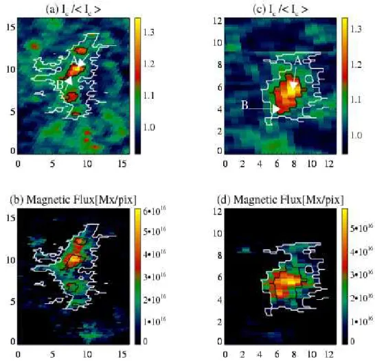
Here we focus on majority polarity magnetic patches with polar faculae. We find that the patches with faculae are not uniformly bright but instead contain smaller faculae. Figure 2.5 shows two examples of patches with polar faculae. In the first (panel (a)), four faculae are identified in one patch. They differ in size, intensity, and magnetic flux. In most cases, the facular islands enclose the local flux maximum within the magnetic patch (e.g., the two uppermost faculae in panel (b)). In the second patch (panel (c)), only one facula is identified. These examples reflect the general case that the number of polar faculae associated with each patch ranges from one to a few. The faculae have fine structure, with a core and an extended halo region (represented by arrows A and B, respectively, in Figure 2.5).
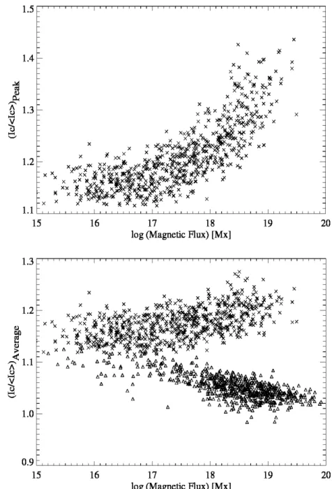
Each magnetic patch is taken to comprise two components: a polar facular region and a nonfacular region. As polar faculae are small structures compared with the nonfacular region within a patch, it is reasonable to use the peak value of Ic/hIci rather than its average value to characterize the faculae, to better cap- ture localized behavior. We refrain from plotting the peak values against flux for nonfacular regions, as it is possible that our threshold might misclassify some true facular pixels as nonfacular. Such errors, if any, could be minimized by taking the average of the normalized continuum intensity. The top panel of Figure 2.6 is a scatter plot of the peak intensity inside the polar faculae versus their mag- netic flux. For each patch, the peak intensity was obtained by considering all the facular pixels in the patch, and the magnetic flux was calculated by summing the flux of all the facular pixels within the patch. There is a clear positive correlation
between the peak intensity and the magnetic flux. For magnetic fluxes ≤1017 Mx, the peak intensity lies between 10% and 20% above the average, beyond which it increases from 20% to 44%. This trend can be explained with the results from Venkatakrishnan (1986), who discovered that convective instability is less efficient for flux tubes with lower magnetic flux (≤1017 Mx). This is a consequence of ef- ficient thermal coupling between smaller flux tubes and the ambient nonmagnetic atmosphere, which hinders convective collapse. Observational confirmation of this finding was given by Solanki et al. (1996) using quiet-Sun data near disk center. Hence, the faculae need to have minimal magnetic flux to be visible as distinct magnetic features.
In the bottom panel of Figure 2.6, we map the normalized intensity averaged over facular (crosses) and nonfacular (triangles) regions against their respective fluxes. The average intensity of the faculae increases with magnetic flux, as ex- pected. A comparison of the two panels makes clear that for faculae, peak intensity is better correlated than average intensity with the magnetic flux. The bottom panel also shows that the average intensity of nonfacular regions decreases with magnetic flux. This bimodal distribution is essentially the same for different µ- ranges. For a given flux value, there exist both bright facular and darker nonfacular regions. Hence, magnetic flux cannot be used to discriminate between facular and nonfacular regions within a magnetic patch. Note that the branching becomes evident at fluxes greater than 1017 Mx. The magnetic patch with large magnetic flux is larger in size and hence it is likely that the nonfacular region in such mag- netic patch will mostly be occupied by granules . We think this is the reason why the average intensity of the nonfacular region approaches unity with increasing magnetic flux.
2.3. RESULTS 25
In Figure 2.7, we plot the probability distribution functions (PDFs) of intrinsic field strength averaged over facular and nonfacular pixels within each magnetic patch. The average field strength of the polar faculae displays a broad peak at 700–1000 G. The nonfacular regions exhibit a peak around 400 G. Since the degree of the depression of the visible surface in a flux tube depends on the intrinsic magnetic field strength, this sharp difference is consistent with the picture set forth by Spruit (1976; see Section 4).
Figure 2.7 also shows, however, that some faculae have very small average intrinsic magnetic field strengths. The field strength may decrease toward the limb as a result of our viewing greater heights in the atmosphere, thus leading to weaker observed fields. In this case, the low values of magnetic field strength would correspond to those from smaller µ. Our examination did not identify any trend in this relationship. We also found that the average intensity of these faculae does not show any dependence on the intrinsic field strength averaged over the respective facular pixels. It is not clear whether these represent different evolutionary phases of faculae, and so to clarify the situation, it will be necessary to examine the temporal evolution of the magnetic patches.
The PDFs of the zenith angles of the magnetic field vectors averaged over facular and nonfacular pixels within each magnetic patch are shown in Figure 2.8. The vectors of both regions are nearly vertical to the local normal, but those of nonfacular regions appear to be slightly inclined. The PDF of the zenith angle has a peak at approximately 169◦ for facular regions and a maximum around 165◦ for nonfacular regions. This small but clear difference may reflect a tendency of faculae to be located in a less diverging portion of the fanning-out field lines (Tsuneta et al. 2008a) of magnetic patches.
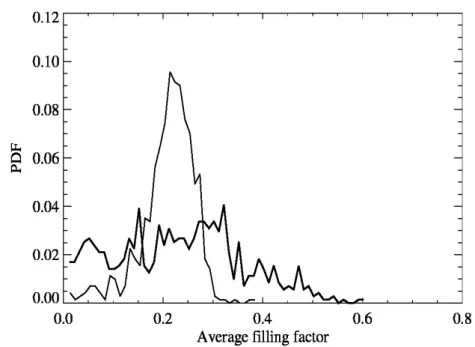
The PDF of the average filling factor for polar faculae shows a broad distri- bution ranging from 0.1 to 0.6 (Figure 2.9), while the nonfacular regions have a distinct peak at ∼0.2. Although some polar faculae have a very high filling fac- tor, there exists no significant difference between facular and nonfacular regions within magnetic patches as compared with the intrinsic field strength or the zenith angle of the magnetic field vector, as is evident from Figures 2.7 and 2.8. Figure 2.10 depicts the variation with µ of the average intensity of polar facular regions within each magnetic patch. The intensity decreases gradually toward the limb, consistent with Okunev & Kneer (2004).
2.3.2 Minority Polarity Patches
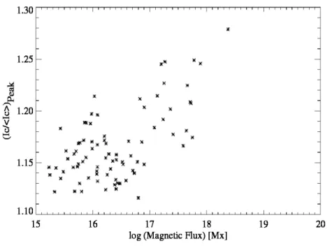
We find that polar faculae are associated with minority polarity patches as well, which is to say, they are polarity independent. However, faculae with minority polarity are very limited in number, and most have magnetic fluxes below 1018 Mx. Figure 2.11 is a scatter plot of the peak intensity of minority polarity faculae as a function of their magnetic flux. This should be compared with Figure 2.6 (top panel), for the majority patches. Peak intensity appears to have a positive correlation with magnetic flux. This indicates that irrespective of polarity both minority and majority polarity faculae exhibit similar behavior.
2.4 Discussion
We have found that polar magnetic patches have substructure, with one or more small faculae embedded in the much larger patches. The faculae appear to be a subregion of magnetic patches. Their shapes inside the patches are irregular. Most
2.4. DISCUSSION 27
Figure 2.5: Two examples of magnetic patches associated with polar faculae: (a, c) normalized continuum intensity; (b, d) magnetic flux in units of maxwell per pixel. White contours enclose the patches, and black contours enclose the polar faculae within the patch. The x and y axes are in arcseconds. For patch 1 (left), the magnetic flux is 3.07 × 10¹⁹ Mx, and µ ≈ 0.26; for patch 2 (right), the flux is 2.24 × 10¹⁹Mx, and µ ≈ 0.21. Arrows indicate core (A) and extended (B) regions of the faculae.
Figure 2.6: Top: Peak value of the normalized continuum intensity Ic/hIci of ma- jority polarity polar faculae vs. magnetic flux summed over facular pixels within each magnetic patch. Bottom: Scatter plot of the average value of Ic/hIci of ma- jority facular (crosses) and nonfacular (triangles) regions as a function of magnetic flux integrated over the respective pixels within each patch. Peak and average in- tensities of polar faculae are calculated over all the facular pixels identified within each patch. For each patch, the average intensity of the nonfacular region is de- termined by taking the mean of intensity of all the pixels outside faculae within that patch.
2.4. DISCUSSION 29
Figure 2.7: PDFs of average intrinsic field strength of polar facular (thick solid line) and nonfacular (thin solid line) regions within magnetic patches. The bin size is 50 G.
Figure 2.8: Same as Figure 2.7, but for average zenith angle. The bin size is 2◦.
Figure 2.9: Same as Figure 2.7, but for average filling factor (see Section 2) The bin size is 0.01.
Figure 2.10: Scatter plot of the average normalized continuum intensity of polar faculae as a function of µ. The lower boundary of the distribution is due to the 4 σ threshold.
2.4. DISCUSSION 31
Figure 2.11: Same as the top panel of Figure 2.6, but for minority polarity faculae.
of the large magnetic concentrations, which have cyclic behavior, host faculae. We also found that faculae exhibit a tendency to have higher intrinsic magnetic field strengths compared with the nonfacular regions inside the associated magnetic patches. Table 2.1 lists the ratio of the magnetic flux of the faculae to that of the patches (including those without polar faculae). We find that less than 20% of the total magnetic flux from the large concentrations is accounted for by the associated faculae. It is important to study the cyclic variation of the facular flux contribution to the large concentrations in order to understand the exact relationship between polar faculae and the solar cycle.
We found that minority polarity faculae also exist in the polar region. The number of minority polarity faculae might depend on the strength of the unipolar field in the polar region. Hence, for weak solar cycles, care should be exercised in assuming that the count of polar faculae (which have been presumed to be unipolar
in most previous studies) is linearly related to the total signed polar magnetic flux. We expected in this investigation to find controlling parameters and/or envi- ronment that switch polar faculae on or off. Intrinsic magnetic field strength and magnetic flux indeed correlate well with the existence of polar faculae, as shown in Section 2.1, but the correlation is somewhat ambiguous, as shown respectively in Figures 2.7 and 2.4. Polar faculae possess stronger and more vertical fields than their surroundings within a magnetic patch. This tendency may be due to the polar faculae being located near the patch centers.
Our observation that faculae possess strong vertical magnetic fields with av- erage intensity decreasing toward the limb is consistent with the hot-wall model (Spruit 1976), which attributes the enhanced brightness of faculae to a depression in the visible surface caused by magnetic pressure, allowing an enhanced view of the hot wall of the flux tube at oblique angles.
We do not have information on the evolution of polar faculae during the de- velopment of the parent magnetic patches from just the snapshot slit-scan obser- vations. It remains necessary to investigate the temporal evolution of magnetic patches and polar faculae to further constrain the properties of faculae.
Chapter 3
Photospheric Flow Field Related
to the Evolution of Polar
Magnetic Patches
3.1 Introduction
The Sun’s polar caps are dominated by unipolar magnetic patches which possess magnetic fields in kilogauss range. According to current understanding, origin of magnetic flux in the polar region is the surplus flux from the decayed active regions transported to the polar cap via diffusion and meridional flow. Precisely how these incoming flux fragments are concentrated into patches or how they decay are not yet studied.
Transportation and concentration of magnetic flux by converging horizontal flows leading to the formation of magnetic structures are observed in the lower heliographic latitudes. Many of the dynamic phenomena observed on the Sun are
33
also the result of interaction of magnetic field with plasma flows. Most of the magnetic flux outside sunspots is concentrated and organized into a variety of multi-scale magnetic features by convective flows in the solar surface layers. The horizontal converging flows concentrate vertical magnetic flux predominantly at the convective cell boundaries. The magnetic flux is advected to the cell bound- aries until the field strength reach the equipartition value which corresponds to the balance between magnetic pressure and dynamic pressure of the convective flows. Further intensification of magnetic fields to kG strengths is induced by the mechanism of convective collapse (Parker 1978; Spruit 1979).
Magnetic fields and photospheric plasma motions are well coupled and hence it is important to understand whether the flow field play any role in the forma- tion and evolution of the polar magnetic patches. This information might give some insight to understand the mechanism involved in polar field reversal and the dynamical processes that could influence the overlying atmospheric layers. In this chapter we investigate the role of photospheric flow fields in the formation and evolution of polar magnetic patches. We also attempt to obtain precursor to the facula appearance within the patch. We used high spatio-temporal reso- lution observations obtained with the Spectropolarimeter(SP) of SOT/Hinode for this study. Section 3.2 describes our observation and analysis.The main results obtained are detailed in section 3.3 and summary and discussion on the results are given in section 3.4.
3.2. OBSERVATIONS 35
3.2 Observations
The data sets used in this study are given in Table 3.1. These data were taken from the north and south polar caps of the Sun with spectropolarimeter (SP) of the SOT aboard Hinode. The SP recorded full Stokes spectra of the two Fe I lines at 630.15 nm and 630.25 nm with the fast map mode whose slit-scanning step is 0.32′′ and integration time in each step is 3.2s. The slit was along N - S direction. The spatial sampling along the slit is 0.32′′ and the spectral sampling is 2.15 pm. Image sequences were obtained with a cadence of 16 minutes and the FOV was 80′′ x 164′′. The observations were taken in such a way that the solar limb and the pole is always within the FOV (e.g., left panel of Figure 3.2). The noise level σ is estimated from the continuum in the Stokes V spectrum and is 1.3 x 10⁻³Ic, where Ic is the continuum intensity. The inversion was performed only for those pixels with Stokes Q, U or V peak is larger than 5σ. Consecutive SP image frames are then aligned using spatial cross-correlation of the Stokes V maps, with pixel accuracy to compensate for the the image motion induced by the correlation tracker device on board the satellite. The spatial offsets thus obtained were used to register other relevant parameters.
To determine the solar limb position, a filtergram (NFI/SOT) image taken at time close to the time of scanning of the center of FOV of the first frame of the SP observations was used. The FG data (shuttered Stokes I and V ) were taken at 140 m˚A red-ward of the Na i D1 5896˚A line center with a FOV of 327.7′′x 163.8′′(see Figure 3.1). The pixel size was 0′′.16 and the the exposure time was 0.205 s. The fg prep.pro procedure in the SolarSoftWare (SSW) package was used to subtract the bias and dark current of FG data. The solar limb position was then estimated
using the FG Stokes I image and was then fitted with a circle to calculate the pole positions. We used the large FOV FG image to obtain solar limb as it is required to minimize the error while fitting the limb with a circle to determine the pole position. FG and SP Stokes V (first scan of the observation) maps were then aligned using spatial cross-correlation to get the information on the limb and pole positions in the SP image scale (see Figure 3.2). This information is used to derive µ (cosine of the heliocentric angle) which is used to obtain the normalized intensity (Ic/hIci).
Table 3.1: SP Observations
Date Time
Center of FOV of the First Scan
Number of Frames
Number of Patches Selected (UT)
2013 Nov 11 10:22-16:43 (-15.0′′, 917.4′′) 24 12 2013 Nov 13 09:57-15:51 (-14.9′′, -942.6′′) 24 5 2013 Dec 08 09:00-15:47 (-14.8′′, 917.3′′) 24 10 2013 Dec 11 09:06-15:53 (-15.0′′, -942.5′′) 24 15 2014 Jan 17 09:06-15:53 (-14.9′′, 917.3′′) 24 13 2014 Jan 23 03:05-09:18 (-14.9′′, -958.0′′) 23 13 2014 Mar 08 11:06-17:43 (-14.9′′, -957.8′′) 24 7
The vector magnetic field and normalized intensity (Ic/hIci) for the SP image sequences were obtained as described in section 2.2. The difference, in the calcu- lation of Ic/hIci, from the study in Chapter 2 is that the pixels in the magnetic patches are identified as facular pixels when their normalized intensity is greater than 3σ instead of 4σ. We found, by inspecting the variation of normalized in- tensity with µ that an intensity threshold of 3σ fits best for our current data set. The continuum intensity averaged over the same µ value is denoted by hIci and σ
3.2. OBSERVATIONS 37
0 50 100 150 200 250 300
0
50
100
150
0 50 100 150 200 250 300
0
50
100
150
Figure 3.1: A sample FG Stokes V image (2013 November 11) with full FOV. The x and y axes are in arcsec. Center of FOV: (14.98′′, 910.1′′)
! "! #! $!
!
%!
&!!
&%!
! "! #! $!
!
%!
&!!
&%!
! "! #! $!
!
%!
&!!
&%!
! "! #! $!
!
%!
&!!
&%!
Figure 3.2: Left: Stokes V map of SP (2013 November 11). Right: FG Stokes V image (Figure 3.1) after alignment with the SP map on the left.The x and y axes are in arcsec.
3.2. OBSERVATIONS 39
is the standard deviation of Ic/hIci.
3.2.1 Identification and Tracking of Magnetic Patches
The code developed by Iida (2012), which was used to identify and track network magnetic patches, in quiet Sun near disk center (for details see Iida 2012, Section 2.2.2) is employed here to select and track the polar magnetic patches. The mod- ifications from Iida′s code and conditions used are detailed as follows. Magnetic patches must:
(1) be within the heliocentric latitude band of 70◦ - 80◦ (2) have minimum size of 5 contiguous pixels
(3) have per pixel flux greater than 2 x 1016 Mx (1 sigma value obtained from the magnetic flux distribution)
We identify patches from the magnetic flux map with a clumping method. The clumping method chooses and groups all connected pixels which satisfy the above criteria into a single magnetic patch.
Here we consider a peak granular advective velocity of 1km/s (e.g., Berger et al. 1998) and that the lateral shift due to rotation (∝ sinφ, where φ is the colaitude) is small within the latitude range of 70◦ - 80◦ (see, Benevolenskaya 2007). So the magnetic patches are assumed to undergo a maximum displacement of about 4 pixel size within an interval of 16 minutes (1 km/s x 960 s = 960 km ∼ 4 pixels). The magnetic patches which spatially overlap in consecutive SP frames are marked as identical. The following patches have been eliminated from our samples: (a) patches which were present during the entire observation period, (b) patches which were present at the beginning of the observation, (c) patches which appeared in
the final frame, and (d) patches that are located at a distance shorter than 4Mm from the edge of the FOV. Those samples which were born and disappeared during the period of observation, with minimum life time of 3 frames are chosen. Finally, 75 magnetic patches in total satisfied all the above criteria.
3.3 Results
3.3.1 Lifetime and Magnetic Flux Distribution of the Sam-
ples
Here, we outline the general properties like lifetime and magnetic flux distribution of the 75 magnetic patches chosen as described in Section 3.2.1. The distribution of apparent life-time of the sample magnetic patches is shown in Figure 3.3. Most of the samples have a life time of 32 min (3 frames) and the average life time is about 1 h. Figure 3.4 shows the distribution of time-averaged magnetic flux of the patches. The average magnetic flux is ∼ 1018 Mx. This value is close to the lower limit of the large flux concentration mentioned in Shiota et al. (2012). Majority of the patches have positive polarity since patches with positive polarity are dominant in both the north and the south polar caps during our observation period. The patches with negative polarity (22 patches) come from both north and south polar region. There are many magnetic patches with larger flux which were present during the entire observation period (6 h) and are not considered in this study.
3.3. RESULTS 41
0 50 100 150 200 250
Lifetime [min] 0.0
0.2 0.4 0.6 0.8
Normalized number of Samples
Figure 3.3: Distribution of lifetime for the 75 sample patches selected for this study.
-2 -1 0 1 2
0.00
0.05
0.10
0.15
0.20
0.25
Magnetic Flux [ × 10
18Mx ]
Normalized Number of Samples
Figure 3.4: Histogram of time-averaged magnetic flux of the 75 samples chosen for this study. Distribution of negative polarity patches (minority polarity) is plotted in red color and positive polarity patches (majority polarity) in black color.
3.3. RESULTS 43
3.3.2 Appearance of Faculae within Magnetic Patches
To find out the coincidence of faculae location with other parameters like magnetic field strength, zenith angle, velocity and filling factor within the magnetic patch, all the sample magnetic patches which enclose facula were selected. The LOS velocity within the magnetic patch is determined from zero-crossing of the Stokes V profile. Zero velocity was defined as the average velocity over all the inverted pixels. We made a vertical (north-south) cut along the slit direction within each of the selected patches through their peak facular intensity location and profiles for all the above mentioned parameters along the vertical cut were obtained. An average profile from the individual profiles for each of the parameters is made and is shown in Figure 3.5. The zero position in the x-axis denote the location of the peak intensity of the facula. The profiles show that at the location of the peak intensity, magnetic field peaks, velocity is quite small and is redshifted and the field is more vertical. The filing factor distribution appears to be rather uniform. The non-uniform distribution of the physical parameters within the patch and the fact that magnetic patches enclose localized concentrations of flux might be an indication that a patch is more complex than a single flux tube structure can explain.
To investigate whether any precursor to the facular appearance can be found out from the frame preceding it using the distribution of parameters like field strength, velocity etc. we carried out the following analysis. For the frames with sample patches possessing facula the physical parameters are averaged over the facula pixels. For the patches in the preceding frame which are devoid of facula we performed the average over the magnetic centroid of the patch and its three
-2.0 -1.5 -1.0 -0.5 0.0 0.5 1.0 0.95
1.00 1.05 1.10 1.15
-2.0 -1.5 -1.0 -0.5 0.0 0.5 1.0
0.95 1.00 1.05 1.10 1.15
Ic /< Ic >
a
-2.0 -1.5 -1.0 -0.5 0.0 0.5 1.0
100 200 300 400 500
Bvertical [G]
b
-2.0 -1.5 -1.0 -0.5 0.0 0.5 1.0
0 10 20 30 40
Zenith Angle [deg.]
c
-2.0 -1.5 -1.0 -0.5 0.0 0.5 1.0
0.0 0.2 0.4 0.6 0.8 1.0
VLOS [km/s]
d
-2.0 -1.5 -1.0 -0.5 0.0 0.5 1.0
Relative Position along Slit [arcsec] 0.10
0.15 0.20 0.25 0.30 0.35
Filling Factor
e
Figure 3.5: The profiles of: (a) normalized intensity, (b) vertical magnetic field, (c) zenith angle ((note that inclination of positive polarity field alone is plotted)), (d) LOS velocity, and (e) filling factor along the slit direction averaged over the samples with facula.
3.3. RESULTS 45
neighboring pixels, assuming that facula appearance occur at the strong field loca- tion. Figure 3.6 (a) show that the peak of the intensity distribution increases from about 2% to about 11% of the quiet sun continuum intensity during the interval of 16minutes. The difference in peak field strengths (Fig. 3.6(b)) and inclination (Fig. 3.6(c)) differ only slightly between the two frames during the same interval. The field strength does not show a sudden increase at the time of facula appear- ance as compared to the intensity. Kaithakkal et al. (2013) reported that the polar facula within magnetic patch exhibit fine structure with a core and an extended halo region. Hence, averaging over the facula region, including both the core and the halo region, within a patch might result in reduced field strength. In the both frames magnetic fields are close to vertical. We does not see any significant dif- ference in horizontal Doppler velocity distributions (Fig. 3.6(d)) between the two frames.
3.3.3 Flow Field at the Time of Appearance and Disap-
pearance of Magnetic Patches
Bisector Analysis
Visual inspection of the magnetograms obtained with the SP observation show unipolar appearance and disappearance of the polar magnetic patches. We inves- tigated whether the photospheric flow field around the patches has any role in the appearance and disappearance of the polar magnetic patches. The variation of the flows with height is also examined by the bisector analysis of the Fe i 630.15 nm line profile. This spectral line is less sensitive to the magnetic field (g = 1.67) in comparison with the Fe i 630.25 nm (g = 2.5) line. Though the magnetic sensitive
0.9 1.0 1.1 1.2 Ic /< Ic >
0.0 0.1 0.2 0.3 0.4
Normalized number of Samples
a
0 200 400 600 800
Bvertical [G] 0.0
0.1 0.2 0.3 0.4
Normalized number of Samples
b
0 10 20 30 40
Zenith Angle [deg] 0.0
0.1 0.2 0.3 0.4
Normalized number of Samples
c
-2 -1 0 1 2
VLOS [km/s] 0.00
0.05 0.10 0.15 0.20 0.25
Normalized number of Samples
d
Figure 3.6: Histograms of: (a) normalized intensity, (b) vertical component of the magnetic field strength, (c) zenith angle of the vertical magnetic field (note that inclination of positive polarity field alone is plotted), and (d) LOS Doppler velocity obtained from the Stokes V zero cross point. The histograms in red represent the distribution of parameters within the patch 16 minute before the appearance of the facula and those in black represent the distribution corresponding to the facula pixels.
3.3. RESULTS 47
line is used, the effect of magnetic field on the velocity measurements is assumed to be negligible in the nearly field-free plasma surrounding the magnetic patch. We obtained bisector positions of the line profile at four intensity levels between line core and wing (see Figure 3.7). The formation height decreases with increase in intensity along the line profile. Thus, the bisector level 4, shown in Figure 3.7, forms deeper in the solar photosphere than the bisector level 1. The Doppler ve- locity is calculated as v = (∆λ/λ0) c, where λ0 is 630.15 nm and c is the velocity of light.
The Doppler shift for each bisector level (∆λ) is determined with respect to the reference wavelength position at that level. As we do not have an absolute reference wavelength position, the reference wavelength is determined as follows. For each of the selected sample patch we define a vertical (north-south) slot of height about 96′′in the slit direction, excluding pixels close to the limb, and width same as that of the patch (defined as the difference between maximum and minimum locations of the patch across the slit direction). The spectral line profiles in this vertical slot were then averaged to obtain a mean spectral line profile. The reference wavelength position for each of the bisector levels was calculated at the respective intensity positions from the mean spectral profile. The reference wavelength position at each bisector level was found to vary by about ±0.2 pm (∼ 0.1 km/s) between image sequences in which a given patch is present .
Since we are interested in a relative velocity in the region around the magnetic patches, we defined a reference wavelength which gives an average velocity in the region of our interest. In this study, we defined a sub vertical slot of width same as that of the patch and height ±8′′ from the top and bottom boundary respectively of each patch (Figure 3.8). The velocity averaged over this sub slot is defined as
zero velocity in our study.
6301.2 6301.4 6301.6 6301.8
0.2 0.4 0.6 0.8 1.0 1.2
Wavelength ( Angstrom )
I / I
c3
4
2
1
Figure 3.7: Normalized Stokes I profile of the Fe i 6301.5 ˚A absorption line. The solid vertical line represents the line core position and the asterisks represents the bisector points.
Appearance of Magnetic Patches
In this section we discuss the photospheric flows in and around the 75 magnetic patches during their appearance. We defined t0 as the time when a magnetic feature is recognized as a patch by the clumping algorithm. The velocity profile in and around the patch along the slit direction is obtained as follows. To minimize the effect of noise, the velocity at each position (within the sub vertical slot) along the slit direction is obtained by averaging the Doppler velocity over the width of
3.3. RESULTS 49
!"# ####!$# ##########%# ###$# #######"
&'()*+,-#./01#2!#$%$3#&1#4#5,16
+
0 5 10 15
0
5
10
15
0 5 10 15
0
5
10
15
Figure 3.8: Magnetic flux map of a sample patch at time t0. The solid line encircles the boundary of the patch. The dashed lines mark the edges of the sub vertical slot mentioned in the text. The x and y coordinates are in arcsec.
the sub vertical slot across the slit direction. In general, magnetic patches have a ’ragged’ shape and hence have non-uniform width across the patch. So if the width of the patch is smaller than the width of the slot at a given location within the patch, the average is calculated only over those positions within the patch. This separate treatment for the magnetic patch is performed to understand the nature of the flow velocity in the presence of the magnetic field. The zero velocity is subtracted from the Doppler value obtained at each position along the slit. A sample velocity profile at the bisector level 4 at time t0 is shown in Figure 3.9. The zero position on the x- axis is the location within the patch at which the average intensity becomes maximum. The velocity profile shows dominance of blue shift on the limb-ward side and red shift on the disk center-ward side within a distance of ± 2′′ respectively from the patch boundary. Blue- and red-shifted flows on
the limb- and disk center-ward directions respectively of the patch represent the existence of converging (incoming) flow field. For each patch, we retraced the patch location at time t0 onto the frame at t0-16 min (Figure 3.10). Doppler velocity in the sub vertical slot at t0-16 min is determined using the same method as explained before to examine whether the flow field exhibit any trend prior to the patch appearance around the retraced location. The precursor was not always observed in the magnetograms at t0-16 min.
-10 -5 0 5 10
Relative Position along the Slit [arcsec]
-1.5
-1.0
-0.5
0.0
0.5
1.0
1.5
V
LOS[km/s]
Figure 3.9: The Doppler velocity profile for the magnetic patch shown in Figure 3.8. The position where the average of the normalized intensity becomes maximum within the magnetic patch is defined as 0 in the x axis and the limb is toward right. The vertical dashed lines represent edges of magnetic patch on its limb- ward and disk center-ward side. Positive velocities correspond to flows away from the observer (redshift). The µ value of the magnetic centroid of the patch is 0.31.
3.3. RESULTS 51
0 5 10 15
0
5
10
15
0 5 10 15
0
5
10
15
Figure 3.10: The location of the patch in Figure 3.8 is retraced to the frame at t0-16 min.The dashed contour represents the location of the patch at time t0.
The above procedure is carried out for all 75 samples to get an average flow field around the retraced patch location at t0-16 min at the four bisector levels. Figure 3.11 shows weak converging flow around the retraced location of the patch at t0- 16 min. Figure 3.12 show average Doppler profiles for regions within and around patches at time t0. The plots on the left display that the patch is surrounded by systematic converging flow at all the four bisector levels. The velocity profiles within the patch shows that converging flow continues more or less within the patch. The slight difference in the flow continuity could be due to the difference in two regions: one magnetic and the other nearly non-magnetic. The redshift becomes weaker in the higher layers but the blueshift does not change with height. Considering the patch and its surrounding together, it appears that the horizontal flow is converging to the zero position. The velocity at the zero point is small and is blue-shifted.
The Doppler velocity values on either side of the zero point come from the