Article
Metropolitan Residents’ Preferences and Willingness
to Pay for a Life Zone Forest for Mitigating Heat
Island Effects during Summer Season in Korea
Dong-Hyeon Kim1, Byeong-Il Ahn2,* and Eui-Gyeong Kim3
1 Institute of Agriculture and Life Science, Gyeongsang National University, Jinju 52828, Korea; [email protected]
2 Department of Food and Resource Economics, Korea University, Seoul 02841, Korea 3 Department of Forest Environmental Resources (Institute of Agriculture and Life Science),
Gyeongsang National University, Jinju 52828, Korea; [email protected]
* Correspondence: [email protected]; Tel.: +82-2-3290-3031
Academic Editor: Giuseppe Ioppolo
Received: 20 September 2016; Accepted: 3 November 2016; Published: 10 November 2016
Abstract: Coupled with green house effects, the urban heat island is occurring more frequently, and thus is becoming a serious social problem. In order to elicit policy implications, the current study assesses the economic values on the heat island-mitigating functions of urban forest through choice experiments. The analytical results suggest that metropolitan city residents’ utility can be increased by raising the size of life zone forests which is comprised of street trees, parks in residential regions, and small forests in school zones. The derived marginal willingness to pay for the life zone forests suggest that the respondents are willing to pay $56.68–76.59 for every increase of the urban forest by 1 m2.
Keywords:heat island; choice experiment; urban forests; non-market goods; willingness to pay
1. Introduction
An urban heat island is a metropolitan region of which the temperature is significantly higher than its surrounding areas. The heat island effect is caused by reflections from urban structures such as buildings, concrete or asphalt roads, and bricks which absorb the heat from the sun during daytime [1,2]. Heat island effects are more severe in summer since the duration of sunshine is longer and the amount of solar radiation is greater than other seasons. The heat island significantly influences the energy demand, air quality, and the health of urban dwellers [3,4]. In addition, the heat island is known to be a main factor which causes tropical nights and sleep disorders, and thus, creates stress for urban residents.
For one method of mitigating heat island effects, increasing the size of urban forest, is known to be very effective [5] (Other than forming life zone forest, alternative efforts are also proven to be effective for mitigating heat island effect: installing green or cool roof [6–8], utilizing bioinspired retro-reflective building envelope [9], and changing to white roof [10]). In Korea, however, the extensive increasing or forming forest in urban areas, similar to Central Park in New York or Hyde Park in London, cannot be easily applied since the land price is very high and most of the city lands are occupied by buildings and other constructions. Therefore, in Korea, the average size of per capita urban forest is small (0.4 m2for the metropolitan areas and 7.76 m2for the cities and small towns) relative to the WHO-recommended level of 9 m2. Seoul, the capital of Korea, has only 0.305 m2of per capita urban forest. The low level of urban forest in the metropolitan regions of Korea is due to the high population density compared with scarce city land. To overcome this limitation, the Korean government is investigating other methods
for augmenting green areas in the metropolitan cities. Increases of street trees, parks in residential regions, and small forests in school zones are all alternatives. In Korea, these green areas are known as life zone forests [11] (A life zone forest is defined as a forest that is relatively easy for urban dwellers to access without additional time or cost to reach it [11]).
Life zone forests are a public good since they have positive externalities such as mitigating heat island effects, purifying air, absorbing noise, and so on, but these positive functions are not evaluated and compensated through market mechanisms. Its positive effects are not exclusive and no single person has the incentives to pay for implementing urban forests, and thus, free rider problems arise. This basic nature of life zone forests requires the government to internalize the positive externality, which implies that the forming and increasing of urban forest in life zones has to be performed through the aid of government budgets.
Coupled with green house effects, heat islands in the cities have become more and more serious. These circumstances force the government to take actions including the expansion of urban forests. The role of government and the public sector in providing green infrastructure for adapting to climate change are found in Agrawal [12], Coffee et al. [13], Ford et al. [14], Preston [15], Carmin et al. [16] and Beirbaum et al. [17]. From this context, for eliciting policy implications, the current study assesses the economic values of life zone urban forests. Since there is no market that provides the price information associated with the values of the urban forest mitigating the heat island effects, we use the choice experiment which has been widely used to evaluate the willingness to pay and the consumers’ appreciation for the attributes of the object in question.
The choice experiment was initiated from marketing research which analyzed the consumers’ choices and has been widely applied in many fields such as transportation, health, food consumption, and environmental and ecological economics [18]. In the forest sector, the choice experiment is mainly applied for assessing the economic values of the public functions of forests such as forest recreation [19,20] and biological diversity [21–29]. The choice experiment is also applied to evaluate the potential of non-timber forest products [30]. These studies imply that the choice experiment is the most appropriate methodology for evaluating the various aspects of the functions or services which are generated by forests [28]. In succession to this line of studies, the present study adds to the choice experiment literature on public services of forest by investigating the heat island mitigation-effects of urban forests.
This paper is structured as follows. In the next section, the survey design for choice experiment is being presented. How the questionnaire was constructed and how the data were collected are explained later in this section. The sample characteristics and descriptive statics of the variables are also presented in this section. Section3presents the estimation results. We then compare the estimation results and marginal willingness to pay for the life zone forests across the two different models. Section4elicits the policy implications and makes final conclusions.
2. Materials
2.1. Experimental Design and Variables
object. Similar cases which postulate a function or phenomenon (instead of a commodity) as the object of choice are found in other studies [25,32,33].
The increases in the area of urban forest are proven to be effective for lowering the urban temperature. Previous studies indicated that the increase per capita of urban forest area by 1 m2results in the decrease of the temperature in urban areas by 1◦C to 3◦C [34–40]. By reflecting these studies,
we included the size of urban forest (in the current study, the size of life zone urban forest) as one of the attributes that influence urban heat islands. Previous studies that evaluated the functions of a forest focus on the detail aspects of the forest. However, those studies placed relatively little attention on factors other than the forest itself. Different from these studies, the current paper not only considers the forest but also other factors that influence the mitigation of heat island effects. Heat island effects could be altered according to several aspects of urban forests such as the shape, location, plant variety, tree density, and so on. However, the differences in these detailed aspects of urban forests are not as influential as the other factors such as number of cars, road size, travel costs etc. Thus, we additionally introduced other more influential factors as the attributes in the choice experiment and simplified the attributes relating to forests as “forest area per capita” for evaluating the respondents’ valuation of urban forest for mitigating heat island effects.
Many prior studies show that road size influences albedo, the reflection coefficient is one of the main contributors for increasing the temperature in urban areas [37,41–43]. Thus, we included per car road size as the other attribute to be presented to the respondents for the choice experiment. Aggregated surface area of buildings is another important factor that influences the albedo. However, there are no such data, thus it is hard to determine the levels to be presented in the choice experiment. Therefore, we did not consider this attribute. Instead, we included the number of cars as the attribute related with heat island effects. As presented in the AppendixA, we conducted regression for investigating the relationship between the temperature in urban areas and possible explanatory variables such as per capita urban forest size, per capita number of cars, per capita electricity usage, per capita road size, average wind speed, amount of rainfall, and a dummy variable which represents whether or not the city of interest is located near the coast. The estimation result indicated that per capita forest size, per capita number of cars, per car road size, average wind speed, amount of rainfall, and a location dummy among the employed explanatory variables are statistically significant. The significant impacts of forest size and number of cars on the temperature in urban area are in the same line of the results in the previous studies discussed above. The rainfall, wind speed, and location are not variables that can be controlled by humans, thus these variables were excluded in the questionnaires (The other uncontrollable factors that influence the heat island effect is insolation or amount of sunshine. This variable has a strong negative correlation with rainfall. Thus, in the regression in the AppendixA, we excluded these variables to avoid the multicollinearity problems). Instead, the variable of number of cars which was identified to be significant in the regression analysis was included as one of the attributes for the choice experiment [4,44]. In the questionnaire, based on the regression analysis, we explained the relationships between urban temperature and selected attributes for the choice experiment as follows, in order to help the respondents to understand the questionnaire.
Provided information regarding the relationship between urban temperature and selected attributes:Based on the analysis of using historical data for 50 years from seven metropolitan cities in Korea during the summer, the increase in urban forest area results in significant decreases in the temperature of urban areas, the increase in the number of cars results in significant increases of the urban temperature and the increase in the road size results in significant increases of the urban temperature.
For the attributes of per capita road size and per capita number of cars, we selected three levels for the choice experiment. The averages of these two attributes in the metropolitan regions were set as baselines. For these attributes, since there are no reference levels other than averages that respondents can easily capture the meanings, we simply presented the alternative levels of “larger (more) than average” and “less than average”. The formulation of urban forest in a large scale inevitably requires the area currently occupied by buildings or roads. However, by definition, it is possible to increase the life zone forest without lessening the road sizes or demolishing the buildings. Thus, the combination of attributes that increase the life zone forests and road sizes at the same time is a possible choice option (We might have more insightful results if various aspects of life zone forest such as species, age, and types of trees had been included as the provided attributes in the choice experiment. Non-inclusion of these factors is the limitation of research).
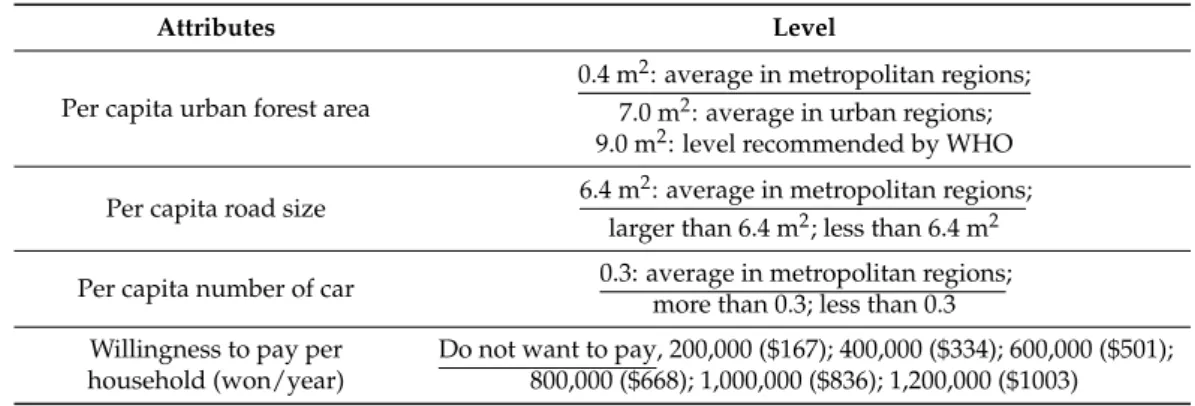
Table 1.Attributes surveyed in the choice experiment.
Attributes Level
Per capita urban forest area
0.4 m2: average in metropolitan regions; 7.0 m2: average in urban regions; 9.0 m2: level recommended by WHO
Per capita road size 6.4 m
2: average in metropolitan regions;
larger than 6.4 m2; less than 6.4 m2
Per capita number of car 0.3: average in metropolitan regions;
more than 0.3; less than 0.3
Willingness to pay per household (won/year)
Do not want to pay, 200,000 ($167); 400,000 ($334); 600,000 ($501); 800,000 ($668); 1,000,000 ($836); 1,200,000 ($1003)
Baseline for each attribute is underlined.
Willingness to pay must be in a form of tax since the object of the choice experiment is not a commodity. Thus, we questioned how much annual tax is willing to be paid per household basis. During 2005 to 2010, Korea Forestry Service spent 185,166 won/household annually for afforesting and managing the forest. Reflecting this budget spending, we posited 200,000 won/household as the minimum for the choice experiment. We then proposed four different taxes per household by allowing equal intervals of 200,000 won (400,000 won/household; 600,000 won/household; 800,000 won/household; and 1,000,000 won/household) and suggested 12,000,000 won/household as a maximum. In 2010, when the survey was conducted, tax per household in Korea was 1,812,000 won/household (based on a four-member household), thus the maximum tax presented in the choice experiment was within the range of actual tax paid by each household. Furthermore, as indicated by Figure1, significant numbers of respondents chose the maximum willingness to pay (i.e., 1,200,000 won/year), thus the range of willingness to pay is designed to be well within the acceptable boundary. We conducted focus group interviews for testing the appropriateness of selected attributes, relevance of the attribute levels, and respondents’ understanding of the questionnaire. The final questionnaire was confirmed after the pretest, which was performed based on the surveys from 50 consumers (of which about 10 percent of the total sample for the main survey) in metropolitan cities.
situation that respondent should respond to 12 different choice sets, we randomly divided 12 choice sets into two blocks and assigned each respondent to one of the blocks. Therefore, six different choice sets were presented to each respondent. Table2shows an example of the choice set that a respondent was faced with.
Figure 1.Distribution of willingness to pay.
Table 2.Example of choice set.
Alternative Option 1 Option 2 Option 3 Option 4
Per capita life zone urban forest (m2)
Average of all cities an d
Do not want to choose any options Average of all cities and
small towns in Korea: 7.0 m2 The level recommendedby WHO: 9.0 m2 Current level: 0.4 m2
Per capita road size (m2)
Current level: 6.4 m Less than current level
Current level: 6.4 m2 Less than current level Larger than current level
Per capita number of cars
Larger than current level
Less than current level Current level: 0.3 Larger than current level Willingness to pay per
household (won/year) 200,000 400,000 1,200,000
We allowed the respondents not to choose the presented options in the choice experiment (i.e., the “no choice option” was included) thus alternative specific constant (ASC), which is specified to be 0 if any of the choice options is selected and 1 if none of the options is selected, was incorporated in the regressions. The coefficient on ASC reveals the attitude towards status quo. In other words, it implies that the taste of respondents is beyond what can be reflected by the attributes presented in the questionnaire.
2.2. Data Collection and Sample Characteristics
The number of respondents for the survey followed Orme [40] (Orme [46] proposed the criteria for selecting the number of respondents as≥c
ta×500, where n is the number of respondents, a is the number of alternatives per task, t is the number of choice tasks and c is the analysis cells). Among the collected data of the surveyed 448 respondents, we excluded the data collected from 14 respondents who did not answer consistently. Thus, a total of 434 samples were used in the analyses.
The questionnaire included the questions related to socio-demographics such as monthly household income, age, housing type, location of residence, types of occupation, employment status, etc. The influences of these socio-demographic characteristics on the choice were estimated in random parameter model (RPL) by allowing the interaction with the dummy formulated by “(1-ASC)”. Table3presents the socio-demographic characteristics of the respondents. Most respondents reside in the city areas, ages 30–59 totaling 65.9 percent; monthly income of 3342–5013 $/month shows the most frequency; and 2–4 member households are of the highest proportion in the sample. These characteristics of age, marital status, household size, and family income are overall comparable to the Korea Census data for the nation.
Table 3.Socio-economic characteristics of the respondents.
Socio-Economic Characteristics Frequency (%) Socio-Economic Characteristics Frequency (%)
Gender Males 237 (54.6) Marriage Single 216 (49.8)
Females 197 (45.4) Married 217 (50.0)
Residential region
Inner city 223 (51.4) Number of family members
below 2 34 (7.8)
Suburb 193 (44.5) 2–4 327 (75.3)
Rural area 18 (4.1) 5–7 73 (16.8)
Housing type
Detached house 101 (23.3)
Occupation
Office job 96 (22.1)
Multi-units house 73 (16.8) Professional 60 (13.8)
Apartment 260 (59.9) Laborer 18 (4.1)
Age (years)
20–29 137 (31.6) Self-employed 48 (11.1)
30–39 124 (28.6) Public officer 63 (14.5)
40–49 98 (22.6) Housewife 89 (20.5)
50–59 64 (14.7) Student 47 (10.8)
60–69 9 (2.1) Unemployed 13 (3.0)
Over 70 2 (0.5)
Residential city
Busan 60 (13.8)
Monthly household income (US $)
Under 1671 26 (6.0) Ulsan 60 (13.8)
1671–3342 139 (32.2) Daegu 60 (13.8)
3342–5013 148 (34.3) Daejeon 60 (13.8)
5013–6683 75 (17.4) Kwangju 60 (13.8)
6683–8354 28 (6.5) Seoul 60 (13.8)
Over 8354 16 (3.7) Incheon 74 (17.1)
3. Estimation Results
3.1. Utility Specification
Unti=β0ASC+ β1FOREST7nti+β2FOREST9nti+β3ROADInti+β4ROADDnti +β5CARInti+β6CARInti
+β7PAYnti+∑rβSEr (1−ASC)×SEn+ εnti
(1)
wherenis the respondent,tis the choice task (t = 1, 2, 3, 4, 5, 6), andiis alternative options 1, 2, 3, and 4. FOREST7andFOREST9denote per capita life zone forest of 7 m2and 9 m2, respectively.ROADIand ROADDare the dummy variables that indicate the increase and decrease of road sizes. CARIand CARDare the dummy variables that indicate the increase and decrease in the number of cars.PAYis the willingness to pay andSErepresents socioeconomic characteristics that include gender, family type, age, family income, residential region, housing type, marital status, and occupation. The estimation of the random parameter logit model is based on the assumption that the coefficients of tastes are independently normally distributed. However, the randomness of taste parameter for price variables could result in a positive estimate which implies an upward-sloping demand curve. Thus, we exclude the heterogeneity for the taste on price as in previous study [47].
3.2. Estimation Results
Figure1indicates the distribution on the willingness to pay of the respondents. The selection of “do not pay” in the presented option shows the highest frequency. The frequencies of the willingness to pay exhibit the negative relationship with the amount of the respondents’ willing to pay, which is a reasonable result. There were significant cases (158 out of 2064 total number of acceptances for the presented willingness to pays) that indicated the maximum willingness to pay as 1003 US dollars (1,200,000 won).
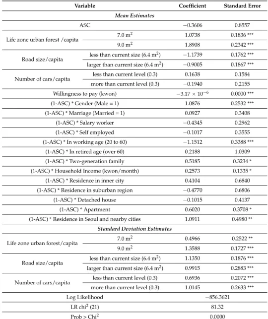
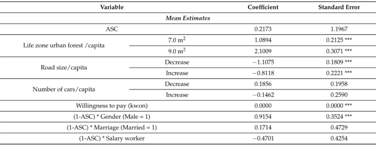
Table4reports estimation results of the RPL model (Estimation results of the RPL allowing interdependence among taste parameters are presented in AppendixB TableB1). For the mean estimates of attributes, the estimated coefficients on per capita life zone forest of 7.0 m2and 9.0 m2 are estimated to be positive and statistically significant at the 1% level. The coefficients that indicate the increase and decrease in per capita road size relative to the current sizes (6.4 m2) are negative and statistically significant at the 1% level. The coefficient on willingness to pay is estimated to be significant at the 1% level, however, the attributes indicating the changes in the per capita number of cars are estimated to have no significance influences on the respondents’ choices. The positive coefficients on the life zone forest suggest that metropolitan city residents’ utility can be increased by increasing the area of life zone urban forest. It is implied that the larger life zone forest would yield more increases in the city residents’ utility, as indicated by the larger coefficient on the life zone forest of 9.0 m2than 7.0 m2.
Interestingly, the coefficients on the decreasing and increasing the road size relative to the current status are estimated to be negative, which implies that the changes in road size would lower the utility of city residents. Decreasing the road size would result in mitigating the heat island effects which would benefit the residents, however at the same time, decreased road sizes would result in more traffic congestion, and thus could be a cost to the residents. The significant and negative coefficient on the attribute of “decreasing road sizes” implies that the residents are more concerned with traffic congestion than the benefit of mitigating heat island effects, especially when they are faced with narrowed roads. Similarly, increases of the road sizes would produce benefits and costs for the residents. In this case, the respondents are also more concerned with the costs, which is the disutility that comes from the worsened heat island, as implied by the significantly coefficient on the attribute of “increasing road sizes”. The comparison on the estimated coefficients of−1.1739 and−0.9005 for the attributes of “decreasing the road sizes” and “increasing road sizes” suggest that the respondents are likely to be more concerned with the disutility caused by the narrowed roads than the widened roads.
two-generation family type, household income, residence in apartment, and Seoul and nearby cities are estimated to have positive influences on the choice of presented option, which can be interpreted that the respondents who have these characteristics are willing to control the heat islands. The respondents of working age show unwillingness to implement the control of heat islands, as indicated by the significantly negative coefficients.
Table 4.Estimation results of Random Parameter Logit Model 1.
Variable Coefficient Standard Error
Mean Estimates
ASC −0.3606 0.8557
Life zone urban forest /capita 7.0 m
2 1.0738 0.1836 ***
9.0 m2 1.8908 0.2342 ***
Road size/capita less than current size (6.4 m
2) −1.1739 0.1762 ***
larger than current size (6.4 m2) −0.9005 0.1867 ***
Number of cars/capita less than current level (0.3) 0.1638 0.1584 more than current level (0.3) −0.1940 0.2155 Willingness to pay (kwon) −3.17×10⁻⁶ 0.0000 ***
(1-ASC) * Gender (Male = 1) 1.0876 0.2532 ***
(1-ASC) * Marriage (Married = 1) 0.0927 0.3408
(1-ASC) * Salary worker −0.4345 0.2962 (1-ASC) * Self employed −0.1017 0.3555 (1-ASC) * In working age (20 to 60) −1.1512 0.3388 ***
(1-ASC) * In retired age (over 60) 0.2188 1.0309
(1-ASC) * Two-generation family 0.5185 0.3234 *
(1-ASC) * Household Income (kwon/month) 0.2573 0.1335 *
(1-ASC) * Residence in inner city 0.4104 0.6840
(1-ASC) * Residence in suburban region −0.4770 0.6806 (1-ASC) * Detached house −0.1015 0.4137
(1-ASC) * Apartment 0.6020 0.3708 *
(1-ASC) * Residence in Seoul and nearby cities 1.0911 0.4980 **
Standard Deviation Estimates
Life zone urban forest/capita 7.0 m
2 0.4966 0.2522 **
9.0 m2 1.3588 0.1727 ***
Road size/capita less than current size (6.4 m
2) 1.1350 0.1876 ***
larger than current size (6.4 m2) 0.9915 0.2883 ***
Number of cars/capita less than current level (0.3) 0.6936 0.2072 *** more than current level (0.3) 1.0145 0.2633 ***
Log Likelihood −856.3621
LR chi2(21) 81.32
Prob > Chi2 0.0000
*, ** and *** indicate significant at 90%, 95% and 99%, respectively.
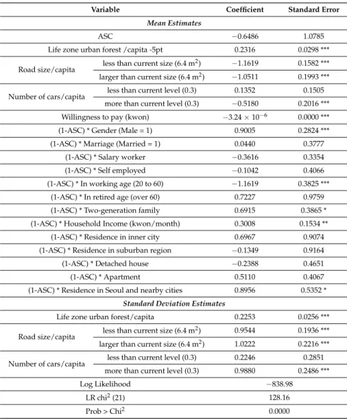
life zone forest is significant at the 1% level. Different from the results in Table4, the coefficient on the attribute of “increasing number of cars” is estimated to be significant at the 1% level. The significantly negative coefficient on this variable implies more cars than the current level will decrease the utility of the respondents. A larger number of cars will result in more traffic congestions and higher urban temperatures, and thus, it is interpreted that residents in metropolitan cities have the unwillingness to accept this option.
Table 5.Estimation results of Random Parameter Logit Model 2.
Variable Coefficient Standard Error
Mean Estimates
ASC −0.6486 1.0785
Life zone urban forest /capita -5pt 0.2316 0.0298 ***
Road size/capita less than current size (6.4 m
2) −1.1619 0.1582 ***
larger than current size (6.4 m2) −1.0511 0.1993 ***
Number of cars/capita less than current level (0.3) 0.1352 0.1505 more than current level (0.3) −0.5180 0.2016 *** Willingness to pay (kwon) −3.24×10⁻⁶ 0.0000 ***
(1-ASC) * Gender (Male = 1) 0.9005 0.2824 ***
(1-ASC) * Marriage (Married = 1) 0.0440 0.3777
(1-ASC) * Salary worker −0.3616 0.3354 (1-ASC) * Self employed −0.1042 0.4066 (1-ASC) * In working age (20 to 60) −1.1619 0.3825 ***
(1-ASC) * In retired age (over 60) 0.7227 0.9759
(1-ASC) * Two-generation family 0.6915 0.3865 *
(1-ASC) * Household Income (kwon/month) 0.3008 0.1534 **
(1-ASC) * Residence in inner city 0.6967 0.9074
(1-ASC) * Residence in suburban region −0.1349 0.9164 (1-ASC) * Detached house −0.2388 0.4651
(1-ASC) * Apartment 0.5110 0.4067
(1-ASC) * Residence in Seoul and nearby cities 0.8956 0.5352 *
Standard Deviation Estimates
Life zone urban forest/capita 0.2253 0.0256 ***
Road size/capita less than current size (6.4 m
2) 0.9544 0.1936 ***
larger than current size (6.4 m2) 1.0222 0.2216 ***
Number of cars/capita less than current level (0.3) 0.2246 0.2851 more than current level (0.3) 0.9880 0.2486 ***
Log Likelihood −838.98
LR chi2(21) 128.16
Prob > Chi2 0.0000
*, ** and *** indicate significant at 90%, 95% and 99%, respectively.
For the estimates of standard deviation, the attributes of life zone forest, changes in road sizes, and increases in the number of cars are estimated to be significant. These results suggest that there are heterogeneities for these attributes, thus the impact of these attributes on the individual respondent’s utility differ according to respondents.
4. Discussion
Marginal Willingness to Pay (WTP) for the Attributes Influencing Heat Island
Using the utility specified in Equation (1), the marginal WTP for each attribute can be calculated asWTP=−βi
changes in road size and the number of cars whileβ6is the estimated coefficient on the willingness to pay.
Table6is the calculations of marginal WTP for each attribute that influences the heat island. Since the changes in number of cars are not estimated to be significant, we excluded the marginal WTP calculations for these attributes. For increasing the life zone forests from the current level (0.4 m2/capita) to 7.0 m2, the respondents have a willingness to pay 447,413 won ($374.09) under the estimation of RPL model 1. For increasing the life zone forests to the level of 9.0 m2, the respondents are willing to pay 787,824 ($658.72). Marginal costs for forming the additional life zone forest will become greater as we form more life zone forest since we will encounter increases in land cost. Thus, it is reasonable that the derived marginal willingness to pay for the larger life zone forests (9.0 m2) is bigger than the lower sized life zone forests (7.0 m2).
Table 6.Marginal willingness to pay for the attribute.
Attribute Marginal WTP
Under RPL Model 1 Under RPL Model 2
Life zone urban forest/capita
7.0 m2 447,413 won ($374.09)
71,474 won1($59.76)
9.0 m2 787,824 won ($658.72)
Road size/capita less than current size (6.4 m
2) −489,126 won ($−408.97) −358,598 won ($−299.83)
larger than current size (6.4 m2) −375,199 won ($−313.71) −324,427 won ($−271.26)
Number of cars/capita More than current level (0.3) — −159,819 won ($−133.69)
1The marginal willingness to pay for the life zone forest of 1 m2/capita.
The derived marginal willingness to pay for the life zone forests imply that respondents are willing to pay 67,790won ($56.68) per 1 m2of life zone forest until it reaches 7.0 m2/capita (Considering the current size of urban forest, the willingness to pay for every additional forest by 1 m2is calculated as 447,4133/(7−0.4) = 67,790). Until the life zone forest reaches 9.0 m2/capita, the respondents have the willingness to pay 91,607 won ($76.59) per 1 m2of urban forest. If we based on the estimation results from the RPL model 2 (i.e., the results in Table6), the marginal willingness to pay for increasing the life zone forest by 1 m2is calculated to be 71,474 won ($59.76), which is within the ranges of the marginal willingness to pay derived from the results in Table4.
Based on the previous studies and regression analysis in the AppendixAwhich investigated the relationships between the urban forest and temperatures in the cities (increasing urban forest by 1 m2/capita results in the decrease in the urban temperature by 1.15 ◦C), we can infer that
respondents' willingness to pay is around 48,663 won ($40.69) to 79,658 won ($66.60) for reducing the temperature in the metropolitan cities by 1◦C during the summer. However, these imputed marginal
willingness to pay are valid when the urban temperature is controlled by only increasing the urban forest, ceteris paribus.
5. Conclusions
The heat island effects have become more serious in many cities and in many countries. One of the effective alternatives for mitigating these effects—the increases of the urban forest—has received much attention. However, the forming of urban forests cannot be achieved through private market mechanisms. Instead, it requires support from the government budget. Installation of green or cool roof and utilizing different materials for building envelopes could be other effective ways of mitigating heat island effects. However, these methods are also hard to pursue in the private sector, therefore market mechanisms are not working, since there is a wide gap between public and private benefit relative to the cost in applying these techniques.
Mitigation of heat island effects provides positive externality since its benefits are not exclusive but no single person has an incentive to pay for mitigating these effects. This situation requires the government to internalize the positive externality through the aid of government budgets. Supporting the installation cost of green or cool roofs would be one of the policies which are implementable to mitigate heat island effect. Governmental increase of urban forest is also an effective policy. The government’s support for green/cool roof installation, however, cannot be applied to all residents or buildings in the cities, because some of buildings are not fit for green roofs and there could a building owner who does not want to change the existing roof. Considering these circumstances, forming life zone forest is a more plausible policy candidate.
For eliciting the policy implications, the current study evaluated the metropolitan residents’ preferences toward forests and derives the willingness to pay for planting additional urban forests within Korea’s metropolitan cities through the form of life zone forests—which include street trees, small parks in residential regions, and green areas in school zones—using the choice experiment.
Different from prior studies which assess the consumers’ willingness to pay for the functions of forest, this paper included the factors that influence heat island effects other than the forest itself. In order to allow the heterogeneities among the respondents, this paper analyzed the random parameter logit model. For designing the choice experiment for the current study, we set “heat island” as the object of choice, and we identified the factors that influence heat island effects in order to comprise them as attributes. Through the reviews of previous studies together with the regression analysis for the relationship between urban temperature and the possible explanatory variables, the road sizes and number of cars were identified as attributes for influencing urban heat islands.
The analytical results indicate that the metropolitan residents’ utility can be significantly increased by forming more life zone forests within the cities. For the changes in the number cars or road size in urban areas, respondents revealed a preference for the status quo rather than increases or decreases of these attributes. Based on the estimated coefficients from the regressions, the marginal willingness to pay for the life zone forests are derived to be $56.68 to $76.59 when increasing the urban forest by 1 m2 per capita.
We expect that the derived marginal willingness to pay for the urban forests can be effectively used for degning the policies associated with lowering the urban temperatures or forming the urban forests. To the best of our knowledge, this is the first attempt that evaluates the values for the heat island-mitigating functions of forest. In this context, we also expect that there will be many succeeding empirical studies that will use the design or framework of the current study.
Acknowledgments: This work was partially supported by the National Research Foundation of Korea Grant funded by the Korean Government [NRF-2014S1A3A2044459].
Author Contributions: Dong-Hyeon Kim and Eui-Gyeong Kim conceived and designed the experiments; Dong-Hyeon Kim performed the experiments; Byeong-Il Ahn and Dong-Hyeon Kim analyzed the data; Byeong-Il Ahn contributed reagents/materials/analysis tools; Byeong-Il Ahn wrote the paper.
Appendix A. Regression Analysis of the Urban Temperature
For identifying the factors that influence the urban temperatures, we set the regression equation as following.
Yit =α 0+α
1Xwindit +α2Xrainit +α3Xitf or+α4Xitcar+α5Xroadit +α6Xitelec+α7Dicoast+εit
whereYitis the temperature at timetin regioni,Xitwindis the wind speed,Xitf oris the per capita urban
forest size,Xrainit is amount of rainfall,Xcarit is per capita number of cars,Xitroadis the road size per capita, Xelec
it is the per capita electricity usage, andDicoastis the dummy which is set to 1 if the city is near coast.
Previous research suggests that urban temperatures are influenced by road sizes and the number of cars [4,32,36–39].
The data of urban temperatures, wind speed, and rainfall were acquired from the AWS (Auto Weather System) in Korea Weather Forest Service. We used the data of urban forest areas, number of cars, and electricity usage in the Korea Statistics Service. The data period is from 1960 to 2010 for the seven metropolitan cities (Seoul, Busan, Kwangju, Daejeon, Incheon, and Ulsan). The temperature data is the average of the temperatures for the summer months (July and August) from 11:00 to 15:00.
Estimation results are reported in TableA1. All explanatory variables other than electricity usage are estimated to be significant at 5% or lower. As we expected, the wind speed, size of urban forest, and rainfall have negative influences on the urban temperatures. Meanwhile, the number of cars and road sizes have positive correlations with urban temperatures.
Table A1.Estimation results of urban temperature.
Variable Coefficient (t-Value) Unit
Constant 28.77 (60.97)
Xwind −0.70 (−5.23) *** m/s Xf or −0.31 (−0.70) *** mm
Xrain −1.15 (−3.98) *** m2/capita Xcar 0.02 (2.45) ** number of car/capita Xroad 0.02 (2.63) ** km2/capita Xelec 0.00 (−0.92) MWh/capita
Dcoast −0.61 (−2.50) ** Dummy (near coast = 1)
R2= 0.85 (Adj.R2= 0.81), *** and ** denote significance at the 1% and 5% level, respectively.
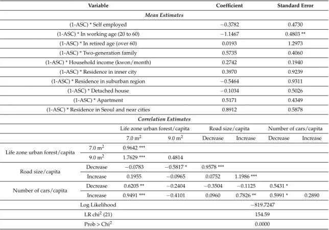
Appendix B. Estimation Results of Random Parameter Logit Model Allowing Interdependence among Taste Parameters
Table B1.Estimation results random parameter logit model with interdependence among taste parameters.
Variable Coefficient Standard Error
Mean Estimates
ASC 0.2173 1.1967
Life zone urban forest /capita 7.0 m
2 1.0894 0.2125 ***
9.0 m2 2.1009 0.3071 ***
Road size/capita Decrease −1.1075 0.1809 ***
Increase −0.8118 0.2221 ***
Number of cars/capita Decrease 0.1856 0.1958
Increase −0.1462 0.2590
Willingness to pay (kwon) 0.0000 0.0000 ***
(1-ASC) * Gender (Male = 1) 0.9154 0.3524 ***
(1-ASC) * Marriage (Married = 1) 0.1714 0.4729
Table B1.Cont.
Variable Coefficient Standard Error
Mean Estimates
(1-ASC) * Self employed −0.3782 0.4730
(1-ASC) * In working age (20 to 60) −1.1467 0.4803 **
(1-ASC) * In retired age (over 60) 0.0193 1.2973
(1-ASC) * Two-generation family 0.5735 0.4060
(1-ASC) * Household income (kwon/month) 0.2742 0.1940
(1-ASC) * Residence in inner city 0.3970 0.9239
(1-ASC) * Residence in suburban region −0.5464 0.9311
(1-ASC) * Detached house −0.1034 0.5026
(1-ASC) * Apartment 0.5171 0.4349
(1-ASC) * Residence in Seoul and near cities 0.8912 0.5878
Correlation Estimates
Life zone urban forest/capita Road size/capita Number of cars/capita 7.0 m2 9.0 m2 Decrease Increase Decrease Increase Life zone urban forest/capita 7.0 m
2 0.9642 ***
9.0 m2 1.7629 *** 0.4814 Road size/capita Decrease
−0.0783 −0.5817 * 0.9578 ***
Increase 0.1955 −0.0965 0.0752 1.1986 *** Number of cars/capita Decrease 0.6205 **
−0.2404 −0.3504 −0.1125 0.5431 *
Increase 0.9491 *** −0.4101 0.0960 0.7826 ** 0.5991 * 0.2890
Log Likelihood −819.7247
LR chi2(21) 154.59
Prob > Chi2 0.0000
*, ** and *** Indicate significant at 90%, 95% and 99%, respectively.
References
1. Oke, T. The energetic basis of the urban Heat island.Q. J. R. Meteorol. Soc.1982,108, 1–24. [CrossRef] 2. Kuttler, W. The urban climate—Basic and applied aspects. InUrban Ecology—An International Perspective on
the Interaction between Humans and Nature; Springer: New York, NY, USA, 2008; pp. 233–248.
3. Rosenzweig, C.; Gaffin, S.; Parshall, L. (Eds.)Green Roofs in the New York Metropolitan Region: Research Report; Institute for Space Studies, Center for Climate Systems Research and NASA Goddard, Columbia University: New York, NY, USA, 2006.
4. Rizwan, A.M.; Dennis, Y.C.L.; Liu, C. A review on the generation, determination and mitigation of Urban Heat Island.J. Environ. Sci.2008,20, 120–128. [CrossRef]
5. Akio, O.; Xin, C.; Takanori, I.; Feng, S.; Hidefumi, I. Evaluating the potential for urban Heat-island mitigation by greening parking lots.Urban For. Urban Green.2010,9, 323–332.
6. Smith, K.R.; Roebber, P.J. Green roof mitigation potential for a proxy future climate scenario in Chicago, Illinois.J. Appl. Meteorol. Climatol.2011,50, 507–522. [CrossRef]
7. Li, D.; Bou-Zeid, E.; Oppenheimer, M. The effectiveness of cool and green roofs as urban heat island mitigation strategies.Environ. Res. Lett.2014,9. [CrossRef]
8. Sharma, A.; Conry, P.; Fernando, H.J.S.; Hamlet, A.F.; Hellmann, J.J.; Chen, F. Green and cool roofs to mitigate urban heat island effects in the Chicago metropolitan area: Evaluation with a regional climate model.Environ. Res. Lett.2016,11. [CrossRef]
9. Han, Y.; Taylor, J.E.; Pisello, A.L. Toward mitigating urban heat island effects: Investigating the thermal-energy impact of bioinspired retro-reflective building envelopes in dense urban settings.Energy Build.2015,102, 380–389. [CrossRef]
10. Sproul, J.; Wan, M.P.; Mandel, B.H.; Rosenfeld, A.H. Economic comparison of white, green, and black flat roofs in the United States.Energy Build.2014,71, 20–27. [CrossRef]
12. Agrawal, A. The Role of Local Institutions in Adaptation to Climate Change. Available online: http://webcache.googleusercontent.com/search?q=cache:e3DMB-W8mAcJ:ipcc-wg2.gov/njlite_download2. php%3Fid%3D8501+&cd=1&hl=ko&ct=clnk&gl=kr (accessed on25 October 2016).
13. Coffee, J.E.; Parzen, J.; Wagstaff, M.; Lewis, R.S. Preparing for a changing climate: The Chicago climate action plan’s adaptation strategy.J. Great Lakes Res.2010,36, 115–117. [CrossRef]
14. Ford, J.; Berrang-Ford, L.; Paterson, J. A systematic review of observed climate change adaptation in developed nations.Clim. Chang.2011,106, 327–336. [CrossRef]
15. Preston, B.; Westaway, R.; Yuen, E. Climate adaptation planning in practice: An evaluation of adaptation plans from three developed nations.Mitig. Adapt. Strateg. Glob. Chang.2011,16, 407–438. [CrossRef] 16. Carmin, J.; Nadkarni, N.; Rhie, C.Progress and Challenges in Urban Climate Adaptation Planning: Results of
a Global Survey; MIT: Cambridge, UK, 2012.
17. Bierbaum, R.; Smith, J.B.; Lee, A.; Blair, M.; Carter, L.; Chapin, F.S., III; Fleming, P.; Ruffo, S.; Stults, M.; McNeeley, S.; et al. A comprehensive review of climate adaptation in the United States: More than before, but less than needed.Mitig. Adapt. Strateg. Glob. Chang.2013,18, 361–406. [CrossRef]
18. Hoyos, D. The state of the art of environmental valuation with discrete choice experiments.Ecol. Econ.2010, 69, 1595–1603. [CrossRef]
19. Arnberger, A.; Haider, W. Social effects on crowding preferences of urban forest visitors. Urban For. Urban Green.2005,3, 125–136. [CrossRef]
20. Rosenberger, R.S.; Needham, M.D.; Morzillo, A.T.; Moehrke, C. Attitudes, willingness to pay, and stated values for recreation use fees at an urban proximate forest.J. For. Econ.2012,18, 271–281. [CrossRef] 21. Bie´nabe, E.; Hearne, R.R. Public preferences for biodiversity conservation and scenic beauty within
a framework of environmental services payments.For. Policy Econ.2006,9, 335–348. [CrossRef]
22. Christie, M.; Hanley, N.; Hynes, S. Valuing enhancements to forest recreation using choice experiment and contingent behaviour methods.J. For. Econ.2007,13, 75–102. [CrossRef]
23. Zandersen, M.; Termansenc, M.; Jensen, F.S. Evaluating approaches to predict recreation values of new forest sites.J. For. Econ.2007,13, 103–128. [CrossRef]
24. Meyerhoff, J.; Liebe, U.; Hartje, V. Benefits of biodiversity enhancement of nature-oriented silviculture: Evidence from two choice experiments in Germany.J. For. Econ.2009,15, 37–58. [CrossRef]
25. Adams, D.C.; Bwenge, A.N.; Lee, D.J.; Larkin, S.L.; Alavalapati, J.R.R. Public preferences for controlling upland invasive plants in state parks: Application of a choice model.For. Policy Econ. 2011,13, 465–472. [CrossRef]
26. Rossi, F.J.; Carter, D.R.; Alavalapati, J.R.R.; Nowak, J.T. Assessing landowner preferences for forest management practices to prevent the southern pine beetle: An attribute-based choice experiment approach. For. Policy Econ.2011,13, 234–241. [CrossRef]
27. Upton, V.; Dhubháin, G.N.; Bullock, C. Preferences and values for afforestation: The effects of location and respondent understanding on forest attributes in a labelled choice experiment.For. Policy Econ.2012,23, 17–27. [CrossRef]
28. Olschewski, R.; Bebi, P.; Teich, M.; Hayek, U.W.; Grêt-Regamey, A. Avalanche protection by forests—A choice experiment in the Swiss Alps.For. Policy Econ.2012,15, 19–24. [CrossRef]
29. Vecchiato, D.; Tempesta, T. Valuing the benefits of an afforestation project in a peri-urban area with choice experiments.For. Policy Econ.2013,26, 111–120. [CrossRef]
30. Boxall, P.C.; Murray, G.; Unterschultz, J.R. Non-timber forest products from the Canadian boreal forest: An exploration of aboriginal opportunities.J. For. Econ.2003,9, 75–96. [CrossRef]
31. Riera, P.; Giergiczny, M.; Peñuelas, J.; Mahieu, P.A. A choice modelling case study on climate change involving two-way interactions.J. For. Econ.2012,18, 345–354. [CrossRef]
32. Xu, W.; Lippke, B.R.; Perez-Garcia, J. Valuing biodiversity, aesthetics, and joblosses associated with ecosystem management using stated preferences.For. Sci.2003,49, 247–257.
33. Thiene, M.; Meyerhoff, J.; Salvo, M.D. Scale and taste heterogeneity for forest biodiversity: Models of serial nonparticipation and their effects.J. For. Econ.2012,18, 355–369. [CrossRef]
34. Ca, V.T.; Asaeda, T.; Abu, E.M. Reductions in air-conditioning energy caused by a nearby park.Energy Build.
1998,29, 83–92. [CrossRef]
36. Ashie, Y.; Thanh, V.C.; Asaeda, T. Building canopy model for the analysis of urban climate. J. Wind Eng. Ind. Aerodyn.1999,81, 237–48. [CrossRef]
37. Taha, H.; Konopacki, S.; Gabersek, S. Impacts of large scale modifications on meteorological conditions and energy use: A 10-region modeling study.Theor. Appl. Climatol.1999,62, 175–85. [CrossRef]
38. Kikegawa, Y.; Genchi, Y.; Yoshikado, H.; Kondo, H. Development of a numerical simulation system toward comprehensive assessments of urban warming countermeasures including their impacts upon the urban buildings, energy demands.Appl. Energy2003,76, 449–466. [CrossRef]
39. Tong, H.; Walton, A.; Sang, J.; Chan, J.C.L. Numerical simulation of the urban boundary layer over the complex terrain of Hong Kong.Atmos. Environ.2005,39, 3549–3563. [CrossRef]
40. Kikegawa, Y.; Genchi, Y.; Kondo, H.; Hanaki, K. Impacts of city-block-scale counter measures against urban heat island phenomena upon a building’s energy consumption for air conditioning.Appl. Energy2006,83, 649–668. [CrossRef]
41. Yamamota, Y. Measures to Mitigate Urban Heat Islands. Available online: http://data.nistep.go.jp/dspace/ bitstream/11035/2703/1/NISTEP-STT018E-65.pdf (accessed on 10 September 2007).
42. Takebayashi, H.; Moriyama, M. Surface heat budget on green roof and high reflection roof for mitigation of urban heat island.Build. Environ.2007,42, 2971–2979. [CrossRef]
43. Ihara, T.; Kikegawa, Y.; Asahi, K. Changes in year round air temperature and annual energy consumption in office building areas by urban heat-island countermeasures and energy saving measures.Appl. Energy2008, 85, 12–25. [CrossRef]
44. Urano, A.; Ichinose, T.; Hanaki, K. Thermal environment simulation for three dimensional replacement of urban activity.J. Wind Eng. Ind. Aerodyn.1999,81, 197–210. [CrossRef]
45. Kanninen, B.J. (Ed.) Valuing Environmental Amenities Using Stated Choice Studies; Springer: Dordrecht, The Netherlands, 2007.
46. Orme, B. Sample Size Issues for Conjoint Analysis Studies, Sawtooth Software Technical Paper. Available online: http://www.sawtoothsoftware.com/support/technical-papers/general-conjoint-analysis/ sample-size-issues-for-conjoint-analysis-studies-2009 (accessed on 10 June 2013).
47. Gao, Z.; Schroder, T.C. Effects of Label Information on Consumer Willingness-to-Pay for Food Attributes. Am. J. Agric. Econ.2009,91, 795–809. [CrossRef]