Doctoral Thesis
Comparative study of various probes of
CP violation in the Higgs sector
Author: Kai Ma
Supervisor: Prof. Kaoru Hagiwara
A thesis submitted in fulfilment of the requirements for the degree of Doctor of Philosophy
in the
KEK Theory Center
Department of Particle and Nuclear Physics School of High Energy Accelerator Science
December 2015
Contents i
Declaration of Authorship iii
Abstract iii
Acknowledgements vii
List of Figures viii
List of Tables xii
1 Introduction 1
2 Probing CP violation in h! (`¯`)(`0`¯0) at the LHC 4
2.1 CP violation in the di-vector bosons decay of Higgs . . . 5
2.1.1 Parameterization . . . 5
2.1.2 CP observables . . . 7
2.2 Helicity amplitudes of h! V1V2 ! (`1`¯1)(`2`¯2) . . . 10
2.3 Helicity amplitudes of photon conversion . . . 14
2.4 Angular resolution . . . 21
2.5 Numerical results . . . 24
2.5.1 h! γ?γ? ! (`+`−)(`+`−) via internal splitting . . . 24
2.5.2 h! Zγ?! (`+`−)(`+`−) . . . 26
2.5.3 h! γγ and h ! Zγ via γ ! e+e− conversion . . . 27
2.5.4 Interference betwwen h! ZZ? and h! Zγ. . . 28
3 Probing CP violation in h! ⌧−⌧+ at the LHC 39 3.1 Parameterization of the h⌧ ⌧ interactions . . . 40
3.2 Helicity Amplitude in the Higgs rest frame. . . 41
3.3 Helicity amplitudes in the ⇡+⇡− rest frame . . . 44
3.4 Reconstruction algorithm . . . 47
3.5 Numerical results . . . 50
4 Probing CP violation in e+e− production of the Higgs boson and to- ponia 55 4.1 Effective t− ¯t− h vertex . . . 57
i
4.2 Helicity amplitudes . . . 62
4.2.1 Factorization and Projection of the helicity amplitudes. . . 63
4.2.2 Production helicity amplitudes . . . 65
4.2.3 Helicity amplitudes of the toponium decay . . . 72
4.2.4 Total Helicity amplitudes and CP observables . . . 75
4.3 Radiative corrections near the threshold region . . . 77
4.4 Numerical results . . . 80
5 Summary 90 A MSSM Higgs sector with loop induced CP violation 95 A.1 The effective Lagrangian of H ! γγ and H ! γZ in the SM . . . 95
A.2 The effective Lagrangian of H! γγ, H ! γZ, A ! γγ and A ! γZ in the two Higgs doublet model with decoupling limit . . . 97
A.3 The effective Lagrangian of H! γγ, H ! γZ, A ! γγ and A ! γZ in the MSSM with decoupling limit . . . 98
B Spinor and vector wave functions 100 B.0.1 Spinor wave functions in Dirac Representation . . . 100
B.0.2 Vector wave functions and Wigner-D functions . . . 101
Bibliography 102
The Graduate University for Advanced Studies (Sokendai)
Abstract
KEK Theory Center
Department of Particle and Nuclear Physics School of High Energy Accelerator Science
Doctor of Philosophy
The Graduate University for Advanced Studies by Kai Ma
Higgs particle is one of the most important ingredients of the Standard Model. It breaks the electroweak vacuum, and generates the mass of both electroweak bosons and matter particles. A similar scalar particle possessing these physical properties has been observed at about 125GeV by both ATLAS and CMS collaborations at CERN in 2012. However, it has not been so clear that whether the observed particle h(125) is the Higgs boson of Standard Model, or the model needs some extensions. So further investigations on the physical properties of h(125) are crucial for the understanding of physics.
CP symmetry of the h(125) is one of the most important properties that has not been understood well. While only one scalar particle is predicted in the Standard Model, many of its extensions not only modify the Higgs couplings to electroweak bosons and fermions, but additional scalars and pseudo-scalars are also predicted. So CP violation effects could be appear naturally through the mixing among these particles. Even through the experimental results disfavor a pure CP odd particle at about 3σ level, large mixing is still allowed in general. In this thesis we study the CP violation effects in the Higgs sector.
There are many channels in which the CP violation effects could appear. In the process of Higgs decaying into two vector bosons, either Z or photon, the CP violation effects appear in the azimuthal angle correlations. This correlation could be measured by ob- serving the leptons from the subsequent decay of these two gauge bosons. However, the leptons are highly boosted because of the large mass of Higgs, so resolving the corre- lation in the transverse plane is still challenging, particularly for the electrons coming from the photon conversion. Similar correlation appears in the production channels via the vector bosons fusion. In this case the CP violation effects could be measured by analyzing the tagged jets or leptons in the final states. The main problem is the huge
QCD backgrounds which can completely wash out this correlation. However, by using matching technique, the QCD backgrounds could be well predicted and then significantly enhance the experimental sensitivity.
We investigate CP violation effect in the Higgs sector via h! 4l channels at the LHC14. Measuring CP violation effect through h! ZZ⇤ ! 4l process is completely impossible because of the dominant CP even contributions. In contrast, CP even and odd contri- butions are at the same level in both h! Zγ ! 4l and h ! γγ ! 4l decay channels. In this paper we study to which level the CP violation effect in the spin correlation of final states could be measured via this two processes at the LHC. The polarization of pho- tons from Higgs decay could be measured through the photon conversion and internal splitting processes. However we find the conversion process is completely useless unless the experimental precision could be improved by a factor of 4. On the other hand the internal splitting channels provide a hope even through it is still challenging.
On the other hand, the CP violation effects could be observed in the interactions be- tween the Higgs and fermions, for instances h! ⌧+⌧−, and t¯t production in associated with a Higgs. In the h! ⌧+⌧− channel, observing the CP violation effects is challeng- ing because the neutrinos carry away lots of kinematical informations. However, it is still promising because of the large decay length of ⌧ , by which the decay vertex and impact parameter could be employed to reconstruct the full kinematics. We use the impact parameter and density function of missing transverse energy as well as the den- sity function of the distance between the neutrinos and visible taus decay products to reconstruct the full kinematics event by event. The most likely configuration is obtained by scanning the taus momentums. Within the present experimental resolution, we find very good collinearity between the reconstructed and true kinematics. The experimental sensitivity of is expected to be 0.1 at LHC14 with an integrated luminosity 3 ab−1. In the t¯t production in associated with a Higgs at the ILC with ps = 500GeV, un- der the approximation that the production vertex of Higgs and toponia is contact, and neglecting the P-wave toponia, we analytically calculated the density matrix. We find that the production rate of singlet toponium is highly suppressed, which behaves just like the production of a P-wave toponia. This is because in the singlet case the Higgs can not affect anything except for carrying away some energy, and also the specialty of near threshold region. In case of triplet toponium, the CP property of Higgs can affect the physics significantly. This is because the S-wave triplet toponium can con- tribute even in the pseudo-scalar case, even through the contribution is still small. Three completely independent CP observables, azimuthal angles of lepton and anti-leptons in the toponium rest frame as well as their sum, are predicted based on our analytical results, and checked by using the tree-level event generator. The nontrivial correlations
come from the longitudinal-transverse interference for azimuthal angles of leptons, and transverse-transverse interference for their sum. The azimuthal angle correlation of lep- ton is related to the azimuthal angle correlation of anti-lepton by CP transformation. Most importantly, the interferences between the transverse and longitudinal component require only either lepton or anti-lepton to be reconstructed. Therefore the number of signal events can be enhanced significantly. These three observables are well defined at the ILC, because the rest frame of toponium can be reconstructed directly. Furthermore, the QCD-strong corrections, which are important at the near threshold region, are also studied with the approximation of spin-independent QCD-Coulomb potential.
First and foremost I want to thank my supervisor Kaoru Hagiwara. It has been an honor to be his last Ph.D. student. He has taught me, both consciously and unconsciously, how good elementary particle physics is done, particularly the connection between theories and experiments that is very important for young researcher to be a real physicist. I appreciate all his contributions of time, ideas, and fundings to make my Ph.D. experience productive and stimulating. The joy and enthusiasm he has for his own research was contagious and motivational for me, even during tough times in my Ph.D. pursuit. The members of the KEK theory center have contributed immensely to my personal and professional time at KEK. The group has been a source of friendships as well as good advices and collaboration. I also would like to acknowledge my friend Satyanarayan Mukhopadhyay who is a postdoc at IPMU. We worked together on an MSSM Dark Matter project. I am very much moved by his enthusiastic explanation of Dark Matter physics, as well as by his intensity, willingness to do the analysis and writing the paper. I also would like to acknowledge my senior Junya Nakamura, and my junior Shingo Mori. We worked together and learned much from them. I would like to acknowledge Prof. Osamu Jinnouchi, from whom I learned details about the ATLAS detector. I would like to acknowledge Dr. Hiroshi Yokoya. We worked together on the toponia project, and I learned much from him on physics of top-anti-top production at electron-positron collider. My time at KEK was made enjoyable in large part due to the many friends that became a part of my life. I am grateful for the time I spent with friends at KEK. For this dissertation I would like to thank my referees: Keisuke Fujii, Osamu Jinnouchi, Kaoru Hagiwara, Ryuichiro Kitano, Mihoko Nojiri, and Yutaka Sakamura for their time, interest, and helpful comments.
I gratefully acknowledge the China Scholarship Council for the financial support that made my Ph.D. work possible. My work was also supported partially by the Hanjiang Scholar Project of Shaanxi University of Technology, and I am honored to be a Younger Hanjiang Scholar of Shaanxi University of Technology.
Lastly but not least, I would like to thank my family for all their love and encouragement, and to my parents who raised me with a love of science and supported me in all my pursuits.
Kai Ma KEK Theory Center and Sokendai August 2015
vii
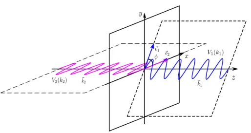
2.1 Definitions of the momenta and polarizations of the two vector bosons. Without loss of generality, the polarization vector of the first vector bosons (with larger virtual mass) is defined to lie on the ˆx direction. . . . 10 2.2 Definitions of the momenta and polarizations of the two vector bosons.
Without loss of generality, the polarization vector of the first vector bosons ( with heavy mass ) is defined to lie on the ˆx direction. . . 11 2.3 Definitions of the momenta and polarizations of the particles. Without
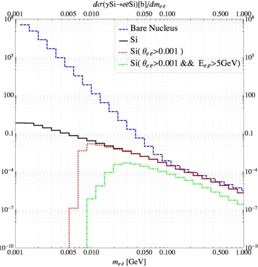
loss of generality, the ˆz-axis is defined along the momentum direction of in-coming photon, ˆx-axis is defined as the polarization direction of the same photon. . . 15 2.4 The blue-dashed line is the distribution for a bare 28Si without any form
factor. The black-solid line is the distribution for a28Si with the form fac- tor Eq. (2.47). The red-dotted line shows the distribution with additional cut on the opening angle ✓cut(e−, e+) = 0.001. The green-dotdashed line is the distribution cut on the opening angle ✓cut(e−, e+) = 0.001, and cut on the lepton energy E(e−), E(e+) > 5GeV. . . 20 2.5 Distributions of the azimuthal angle of leptons which is measured in the
Lab frame. . . 21 2.6 pT dependence of the experimental resolution in azimuthal and polar angle
directions. The red cross points are experimental data taken from Ref. [61]. The solid-blue line is our result by fitting the data. . . 22 2.7 1σ contour plots of the resolution for φ = 0 and several ⌘ = 0.0, 0.5,
1.0, 1.5, 2.0, 2.5. In every plots, dotted-black line is for pT = 10GeV, solid-blue line is for pT = 20GeV and dashed-red line is for pT = 30GeV. 30 2.8 Transverse momentum distributions for process pp! h ! γ(e−e+)γ(e−e+).
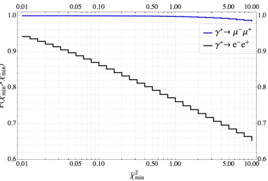
The distributions have been normalized to 1, i.e. half of the number of γ in h ! γγ and half of the number of ` in h ! (`¯`)2. The blue-dotted line shows the pT distribution of virtual photon and the black-solid line shows the pT distribution of electron from virtual photon. . . 31 2.9 The probability of the γ ! `¯` splitting events that satisfy the angular
resolution condition χ2min > ¯χ2min for the process pp! h ! γγ. The blue- solid and the black-solid lines show the probabilities of the cut-off value
¯
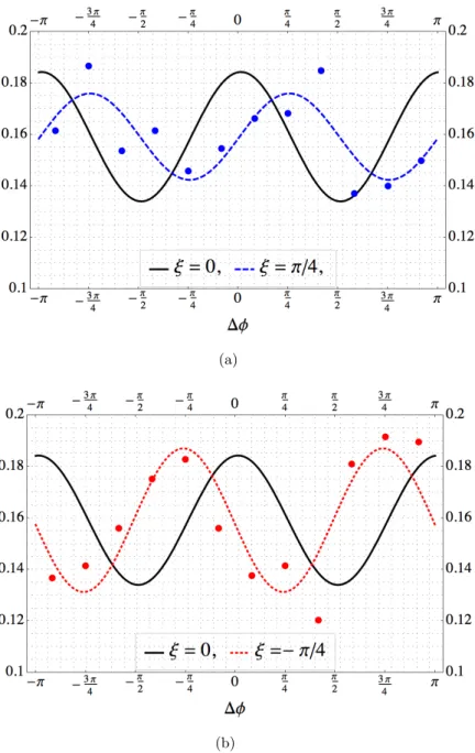
χ2min, respectively, for the γ? ! µ−µ+ and γ?! e−e+ splitting events. . 31 2.10 Azimuthal angle correlations for the process pp ! h ! γγ ! 4` with
(a) ⇠ = ⇡/4 and (b) ⇠ = −⇡/4. As a reference the prediction for the SM Higgs boson is shown by the black dots (and line). The data points correspond to an integrated luminosity 100 ab−1. . . 32
viii
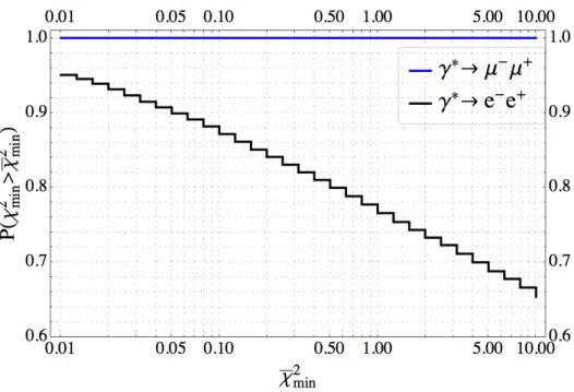
2.11 Transverse momentum distributions for process pp ! h ! Zγ. The solid-green line shows the pTdistribution of Z, the dashed-red line shows the pTdistribution of µ from Z decay, the dotted-blue line shows the pTdistribution of γ and the solid-black line shows the pTdistribution of e from virtual photon. . . 33 2.12 The probability of the γ ! `¯` splitting events that satisfy the angular
resolution condition χ2min > ¯χ2min for the process pp ! h ! Zγ. The blue-solid and the black-solid lines show the probabilities of the cut-off value ¯χ2min, respectively, for the γ? ! µ−µ+ and γ? ! e−e+ splitting events. . . 33 2.13 Azimuthal angle correlations for the process pp ! h ! Zγ ! 4` with
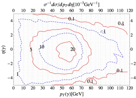
(a) ⇠ = ⇡/4 (blue points and blue-dashed line) and (b) ⇠ = −⇡/4 (red points and red-dashed line). As a reference the prediction for the SM Higgs boson is shown by the black-solid line. The data points correspond to an integrated luminosity 100 ab−1. . . 34 2.14 Contour plot of the normalized production cross section (in unite of 10−3)
in the pT(γ)− ⌘(γ) plane for the process pp ! h ! γγ. The bin size is 5GeV for pT(γ) and 0.2 for ⌘(γ). . . 35 2.15 Contour plot of the normalized production cross section (in unite of 10−3)
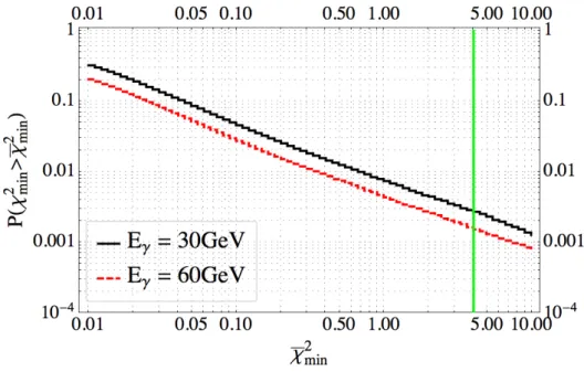
in the pT(γ)− ⌘(γ) plane for the process pp ! h ! Zγ. The bin size is 5GeV for pT(γ) and 0.2 for ⌘(γ). . . 35 2.16 The probability of the ˆγ ! e−e+that satisfy the angular resolution condi-
tion χ2min> ¯χ2min for the BH conversion process γSi! `¯`Si. The pseudo- rapidity of incident photon has been chosen as ⌘(γ) = 0. The black-solid and the red-dashed lines show the probabilities for pT(γ) = Eγ = 30GeV and pT(γ) = Eγ = 60GeV, respectively. . . 36 2.17 Contour plot of the probability of e+e− pair satisfying the angular reso-
lution condition χ2min > 4, as well as pT(e−), pT(e+) > 5GeV for the BH conversion process. For convenience, the values have been enlarged by 104 times. . . 36 2.18 Contour plot of the probability of e+e− pair satisfying the angular res-
olution condition χ2min > 4, as well as pT(e−), pT(e+) > 5GeV for the process pp! h ! γγ. For convenience, the values have been enlarged by 104 times. . . 37 2.19 Contour plot of the probability of e+e− pair satisfying the angular res-
olution condition χ2min > 4, as well as pT(e−), pT(e+) > 5GeV for the process pp ! h ! Zγ. For convenience, the values have been enlarged by 104 times. . . 37 2.20 The black-solid, blue-solid, red-solid lines show the decay width distri-
butions with respect to the invariant mass m2 for h ! Zγ, and the longitudinal and transverse contributions of h! ZZ⇤. The dashed-blue line shows the interference between h ! Zγ and the transverse part of h ! ZZ⇤. The dashed-red line shows the interference between h! Zγ and the longitudinal part of h! ZZ⇤. For the longitudinal interference, since it is zero after the integral, therefore we integrate the azimuthal angle only in the range (0, ⇡/2). . . 38
3.1 Correlation between the true and reconstructed azimuthal angle difference for a maximum mixing, i.e. ⇠h⌧ ⌧ = ⇡/4. The azimuthal angle is calculated in the ⇡+⇡− rest frame. The data points correspond to an integrated
luminosity 1 ab−1. . . 52
3.2 Distributions of the reconstructed azimuthal angle for ⇠h⌧ ⌧ = 0 (blue-solid line) and ⇠h⌧ ⌧ = ⇡/4 (red-dashed line). The azimuthal angle is calculated in the ⇡+⇡− rest frame. The data points correspond to an integrated luminosity 1 ab−1. . . 52
3.3 Distributions of reconstructed azimuthal angle differences for the major background process pp ! Z ! ⌧−⌧+ (blue-solid), and the sum of signal and this background (red-dashed line) in the maximum mixing case ⇠h⌧ ⌧ = ⇡/4. The data points correspond to an integrated luminosity 1 ab−1. . . . 53
4.1 Feynman diagrams that contribute the V − ht¯t effective vertex (labeled by a big gray dot) in the threshold region. This approximation does not depend on the V − t¯t vertex, so V could be either Z or γ. . . 58
4.2 Definitions of the kinematical variables in the e+e− rest frame specified by the axises x− y − z, and the t¯t rest frame specified by the axises x⇤− y⇤− z⇤. In the e−+ e+ rest frame, the electron momentum is chosen along the z-axis and the t¯t momentum lies in the x−z plane with positive x component. In the t¯t rest frame, the negative of the h momentum direction is chosen as the z?-axis, and the y?-axis has the same direction as the y-axis. . . 59
4.3 QCD corrections to the effective V − ht¯t vertex in the threshold region. In this region, summation of an infinite number of diagrams is needed. The big black dot indicates the exact vertex function after this summation. 61 4.4 Definitions of the kinematical variables of tops and leptons in the topo- nium rest frame. The z?and x?axes are specified by the toponium moving direction and the scattering plane in the laboratory frame, respectively. . 72
4.5 Green functions for binding energy E =−2GeV. . . . 81
4.6 Green functions for binding energy E = 0GeV. . . 81
4.7 Green functions for binding energy 2GeV. . . 82
4.8 Green functions for binding energy E = 4GeV. . . 82
4.9 Contour plot of the absolute value of Green functions for S-wave. . . 83
4.10 Contour plot of the absolute value of Green functions for P-wave. . . 84
4.11 Production cross section for pure scalar Higgs with unpolarized beams at ps = 500GeV. The black-dashed line is the cross section of S-wave toponium at Born level. The blue-dash-dotted line shows the rest of the production cross section (which is essentially the P-wave contribution). The red-solid line shows the production cross section after the QCD- Coulomb corrections. . . 85
4.12 Production cross section for pure pseudo-scalar Higgs with unpolarized beams at ps = 500GeV, The black-dashed line is the cross section of S-wave toponium at Born level. The blue-dash-dotted line shows the rest of the production cross section (which is essentially the P-wave contri- bution). The red-solid line shows the production cross section after the QCD-Coulomb corrections. . . 86
4.13 Azimuthal angle correlation for pure scalar (black-solid line) and pseudo- scalar (red-dahsed line). . . 87
4.14 Azimuthal angle correlation for positive maximum mixing (red-dashed line), negative maximum mixing (blue-dotted line), and the reference case of pure scalar (black-solid line). . . 87 4.15 Azimuthal angle correlations of lepton and anti-leptons for pure scalar
Higgs (black-solid line), pure pseudo-scalar (blue-dotted line). . . 88 4.16 Azimuthal angle correlations of lepton and anti-leptons for pure scalar
Higgs (black-solid line), pure pseudo-scalar (blue-dotted line). . . 88 4.17 Azimuthal angle correlations of anti-leptons for mixing case.. . . 89 4.18 Azimuthal angle correlations of lepton for mixing case. . . 89 5.1 Magnitude of tffective HV V and AV V couplings as functions of tan(β)
predicted in MSSM. (normalization is different from the definition in the first section). . . 91 5.2 Relative phase of ⇠γγ and ⇠Zγ as functions of tan(β) predicted in MSSM.
(normalization is different from the definition in the first section).. . . 92
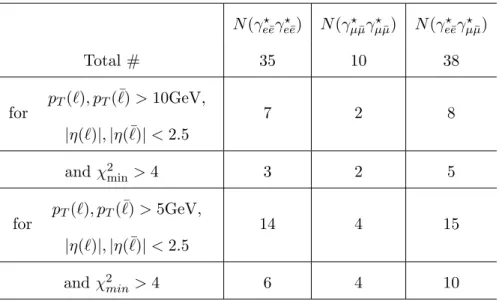
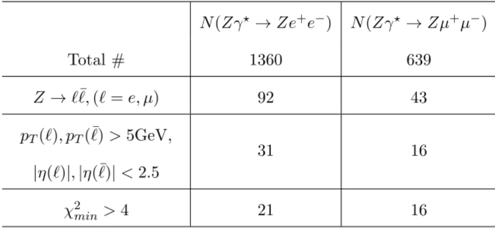
2.1 Number of events for the process pp! h ! Zγ ! 4` after the kinematical cuts. The total number of events are normalized to the SM values with 1 ab−1 of luminosity at HL-LHC(14TeV). . . 24 2.2 Number of events for the process pp! h ! γγ ! 4` after the kinematical
cuts. The total number of events are normalized to the SM values with 1 ab−1 of luminosity at HL-LHC(14TeV). . . 25 2.3 Number of events for the process pp! h ! Zγ ! 4` after the kinematical
cuts. The total number of events are normalized to the SM values with 1 ab−1 of luminosity at HL-LHC(14TeV). . . 26 3.1 Efficiency and number of events of the processes pp ! h/Z ! ⌧−⌧+ !
(⇡−⌫⌧)(⇡+⌫¯⌧) at 14TeV with an integrated luminosity 1ab−1. . . 54 4.1 The Clifford expansion coefficients of the vertex Eq. (4.9). The Bt¯t (B =
γ, Z) vertex is denoted as ΓµB = gVBt¯tγµ + gBt¯Atγµγ5. The momentum qµ= pµ1 − pµ2 is the relative momentum between top and anti-top. . . 60 4.2 Quantum numbers of the standard bi-spinors formed by top and anti-top
in the non-relativistic limit. The bi-spinors are evaluated in the rest frame of t¯t. . . 61 4.3 Quantum states of the total final system. The spin and angular momenta
are summed by first combine the top and anti-top system, and then com- bine the toponim ( t) and Higgs system.. . . 62 4.4 Operators generate toponium in S-wave . . . 68
xii
Introduction
Symmetry, in the early days of sciences, was just a language of interpretation in the study of simple geometric objects. It has only been last century that the importance of symme- try in complex physical systems was gradually being realized since the pioneering work of Wigner and others in atom and nuclear physics. Now days, almost everybody believe that symmetries are so fundamental that all lows of nature are originate in symmetries. Noether proved that every continuous symmetry implies a conserved quantity[1]. The most powerful theory, Electrodynamics, was found to be a result of (continuous) local gauge symmetry[2]. The profound extrapolation of abelian gauge symmetry by Yang and Mills[3], which was initially treated as a just formal product, was realized in a latter time playing essential role in both weak and strong interactions. Discrete symmetry was also never hanged out. It dominates the structure of crystal. Bose-Einstein and Fermi-Dirac statistics, which are the footstones of modern particle physics, are governed by the permutation symmetries.
Nevertheless, just as people were immersed in the beauty of the symmetry, the came symmetry breaking, shocked everyone. The Cooper electron pair[4–6], which can explain the superconductivity in low temperature, was found to be a result of the spontaneous symmetry breaking of local gauge symmetry. Its generalization in the context of quan- tum field theory, which is called Higgs mechanism[7–9], has been proved to be the most profound discovery in elementary particle physics. The parity symmetry, which is dis- crete, is also broken in weak interactions[10, 11]. It was also found that, the classical conservation low from Embedding discrete symmetries into local gauge theories, can be
1
broken at the quantum level[12]. Even through more realistic is the symmetry breaking as it should since we can distinguish one thing from another, nobody ever before rec- ognized that it can have so profound and lasting influences. Now days, nobody talks symmetry without mentioning symmetry breaking. To which degree the symmetry is broken becomes the fundamental question of physics.
Charge conjugate C, parity P, time reversal T symmetries are three of the most funda- mental and relevant ones. Among their combinations, CP occupy a very unique place in elementary particle physics. Apart from the CP violation in the Kaon system (and other hadron systems), we have learnt that our universe also breaks the CP symmetry[14]. On the other hand, talking about C alone is somehow ambiguous because the particle mov- ing forward is equivalent to its anti-particle moving backward. Therefore we could not unambiguously distinguish the particle from anti-particle as long as CP is conserved which breaks this equivalency.
On the other hand, the relativistic quantum field theory is naturally CPT invariant[15]. Therefore CP violation implies the breaking of time reversal symmetry. Furthermore, the time reversal symmetry T in the context of quantum mechanics is an anti-Hermite operator which transforms numbers into their complex conjugates. Therefore breaking of T or CP must be related to some complex parameters in the model. According to the principles of quantum mechanics, any observable in a quantum process, for instance the transition probability, is invariant under a global phase rotation on the transition amplitudes. Therefore only the relative phase among different transition amplitudes can affect the measurements, which is called quantum interference in general. This is similar to the classical phenomena of Young’s double-slit interference where the two slits generate two different path (mimic to different quantum amplitudes) to the detector. There are three kinds of relative phases that can arise in the quantum amplitudes: 1) strong phase, that is defined to be one which has same signs in the transition amplitude for a quantum process and in the transition amplitude for its CP conjugate quantum process; 2) weak phase, that has the same sign in the transition amplitudes for the two CP conjugated quantum processes; 3) spurious phase, which are purely conventional relative phases between an amplitude and the amplitude for CP conjugate process. They just come from the assumed CP transformation of the related quantum states and field operators, and usually are related the some kinematical variables.
The strong, weak phase and spurious phases (here and below we always talk about relative phase) can affect the quantum measurements in different ways. The spurious phase can always be measured because it is related to the kinematical variables that are measured directly. This is not true for the strong and weak phases. Without loss of generality, we assume there are two transition amplitudes, which is the minimal condition to observe quantum interference. Let i and f are the initial and final quantum states, and M1(i! f) and M2(i ! f) are the two amplitudes which cause the transition i ! f. According to the principles of quantum mechanics, the total transition amplitude is the sum of these two,
M(i ! f) = M1(i! f) + M2(i! f) . (1.1) Then the total transition probability is
P (i! f) / |M(i ! f)|2
= X
k=1,2
|Mk(i! f)|2+ 2|M1(i! f)||M2(i! f)| cos(⇠1− ⇠2+ δ1− δ2) , (1.2)
where ⇠k and δk are the weak and strong phases of the two transition amplitudes. On the other hand, the conjugated filed operators can cause quantum transition ¯i! ¯f with a transition probability
P (¯i! ¯f )/ |M(¯i ! ¯f )|2
= X
k=1,2
|Mk(¯i! ¯f )|2+ 2|M1(¯i! ¯f )||M2(¯i! ¯f )| cos(−⇠1+ δ1+ ⇠2− δ2) .(1.3)
Then the CP asymmetry is given by P (i! f) − P (¯i ! ¯f )
P (i! f) + P (¯i ! ¯f ) =
2|M1||M2| sin(⇠1− ⇠2) sin(δ1− δ2)
|M1|2+|M2|2+ 2|M1||M2| cos(⇠1− ⇠2) cos(δ1− δ2)
. (1.4)
Therefore in the case of we are measuring only the total transition rate, observing either one of them requires another one must be non-zero. On the other hand, if we can relate the strong/weak phase to a certain spurious phase which has to a CP-even/odd, then the strong/weak phase can be observed by investigating the distribution of the transition rate with respect to the corresponding kinematical observable of this spurious phase.
Probing CP violation in
h ! (`¯`)(` 0 ` ¯ 0 ) at the LHC
The h ! V V0 ! 4` channels, which are called the golden channels, are promising to measuring the CP violation. The V ! `¯`transition can happen via the internal splitting, and photon conversion if V = γ. In Ref. [23], a maximum likelihood analysis on the h ! V V0 ! 4` was performed for the internal splitting processes. By assuming an overall uniform efficiency 60%, they found the golden channel has the potential to probe both the CP nature as well as the overall sign of the Higgs coupling to photons well before the end of high-luminosity LHC running. However, the most important effects because of the experimental angular resolution, particularly for the internal splitting process of virtual photon, were not analyzed carefully. For the photon conversion process, the CP sensitivity was analyzed with the assumption that Higgs is at rest in the lab frame in Ref. [36].
We study sensitivity of the h(125) ! 4` decay distributions to the CP-odd component of the Higgs boson in various kinematical configurations. The dominant h! ZZ? ! 4` process are found to be least sensitive because of the overwhelmingly large tree-level CP- even amplitudes. Since both CP-even and -odd amplitudes appear in the one-loop order for the h! Zγ and h ! γγ decay channels, we examine carefully the kinematical region where one or both pair of `¯` is near the photon mass shell, in particular the γ ! e+e− conversion process. For the photon conversion process, we include the non-trivial pT and ⌘ distribution of the Higgs by convoluting the production rate and BH conversion
4
probability in the pT and ⌘ plane (because of the symmetry of detector, the azimuthal angle direction is trivial and have been integrated). Once typical angular resolution of e+e− in the LHC detectors is taken into account, the conversion processes are strongly suppressed and found to be useless unless the experimental angular resolution can be improved by a factor of 4. Without takeing into account of the background, we find the experimental sensitivity is about ∆⇠hγγ = 0.33 for pp! γ⇤γ⇤ ! 4`, and ∆⇠hZγ = 0.25
for pp! Zγ⇤! 4`, with an integrated luminosity 3 ab−1.
2.1 CP violation in the di-vector bosons decay of Higgs
Both the ATLAS and CMS have studied the CP property of the new scalar boson in the h! ZZ?decay channel[19–21], and the pure pseudo-scalar assumption is disfavored at more than 3σ. However, if the mass eigenstate h(125) does not have a definite CP, the fraction of its CP-odd component is not constrained effectively effectively because of the smallness of the CP-odd coupling to Z pair, which is loop suppressed, as compared to the CP-even coupling that appear in the tree-level. In this section we first give our parameterization of the couplings and the mixing parameters, and then discuss how to measure the CP violation effects appearing in the h! 4` decay channels.
2.1.1 Parameterization
There is a wide variety of BSMs that could lead to relatively large CP violation in the Higgs sector, such as the Type-I and Type-II 2HDMs, the MSSM and its extensions with or without R-parity violation. In models with two Higgs doublets, we have three neutral real scalar bosons, two of which have CP-even and one CP-odd couplings to quarks and leptons. The observed boson h(125) can be a mixture of the CP-even and CP-odd states in the presence of CP violation, which can be significant in models with CP violating Higgs potential in the tree-level or through large radiative effects.
Motived by the observation that the h(125) couplings do not deviate much from the SM predictions, we introduce the following simple parameterization of the Higgs mixing,
h = p 1
1 +|✏|2(H + ✏A), (2.1)
where H has the CP-even couplings to the weak bosons and the fermions, just like the SM Higgs boson, and A has the CP-odd couplings to quarks and leptons. This is an approximation in generic two Higgs doublet models, where h(125) is a mixture of three real scalars, H, H0, A:
h = UhHH + UhH0H0+ UhAA . (2.2) In the current basis, where H has the SM Higgs boson couplings, the state H0 has no tree-level couplings to quarks, leptons and weak bosons. We therefore find that all the results for CP-odd observables presented in this paper are valid in generic 2HDM’s with the identification
✏= UhA
UhH (2.3)
whereas the normalization of the couplings should be replaced by the parameter p 1
1 +|✏|2 ! |UhH| (2.4)
We nevertheless adopt a single parameterization Eq. (2.1), since it allows us to parametrize the CP-violating effects in the Higgs mixing by a single complex parameter ✏, just like in the neutral K system.
By including the mixing Eq. (2.1), the effective Lagrangian relevant for the h ! 4` process can be expressed as
−L = h
⇢ m2Z 2vp1 +|✏|2Z
µZ
µ+ ¯ghZγ
↵ 4⇡vZ
µ⌫F
µ⌫+ ¯✏hZγ
↵ 4⇡vZ
µ⌫Fe µ⌫
+¯ghγγ ↵ 8⇡vF
µ⌫F
µ⌫+ ¯✏hγγ
↵ 8⇡vF
µ⌫Fe µ⌫
%
. (2.5)
where v = 256GeV is the vacuum expectation value of the SM Higgs boson (H), and
¯
ghV V0 = pgHV V0
1 +|✏|2 , ¯✏hV V0 =
✏gAV V0
p1 +|✏|2 . (2.6)
Here the couplings ¯ghV V0 and ¯✏hV V0 are typically induced in the one-loop order for V V0 = γγ and Zγ, and we normalized to the factor ↵/(4⇡). Note that we do not examine the CP-odd operator for the ZZ channel,
¯
✏hZZ = ↵ 8⇡vZ
µ⌫Ze
µ⌫, (2.7)
since it is obvious that the tree-level mediated h! ZZ channel has little sensitivity to the loop induced physics. In the γγ and Zγ channels, on the other hand, both the CP- even and CP-odd interactions are mediated in the loop-level, and there is a possibility that the CP-even and CP-odd amplitudes have the same order of magnitudes, which is a necessary condition to observe CP violation in the h(125) couplings, even if it has a significant mixture of CP-odd component.
All the measurements of the h(125) couplings are so far consistent with the predictions of the SM Higgs boson, and in particular the hγγ (hZZ and hW W ) coupling strength are even constrained as µhV V = 1.04± 0.13 [29]. In the effective Lagrangian Eq. (2.5), this implies the constraint
p 1
1 +|✏|2 = 1.04± 0.13 , (2.8)
which implies |✏| < 0.7 at the 95% CL. Although the allowed region of |✏| depends on our assumptions, we note here that relatively large mixture of CP-odd component in h(125) is not ruled out by the present measurements, and that there is still a possibility of discovering CP violation in the h coupling.
2.1.2 CP observables
It has been well know that the CP property of the two photon (or two transversely polarized vector boson) system in zero angular momentum (J=0) can be studied by suing their spin correlation, which can e.g. be measured through the vector boson decay (or conversion) into a lepton pair. Historically, the pseudo-scalar nature of ⇡0 meson was established by the e+e− plane correlation in the leptonic conversion process. The helicity amplitude for the decay process h ! Zγ (h ! γγ) is (hear and after we will suppress an overall factor ↵/(2⇡v))
Mλ1λ2 = ¯ghV V0[(k1· "⇤2)(k2· "⇤1)− (k1· k2)("⇤1· "⇤2)] + ¯✏hV V0✏µ⌫↵βk1µk2⌫"⇤1↵"⇤2β , (2.9)
where k1,2µ and "↵1,2 are the momenta and polarization vector of the two vector bosons, see Fig. 2.1. We observe that the CP even interaction makes the polarization vectors of the two vector boson parallel, while the CP odd interaction makes them perpendicular to each other. So in order to observe the CP violation effects, coherent superposition of the two transverse polarization states is necessary.
In the h(125) rest frame we choose the V V0 momentum directions along the z-axis,
k1 = 1 2mh
✓
1 +s1− s2
m2h , 0, 0, β
◆
, (2.10a)
k2 = 1 2mh
✓
1−s1− s2
m2h , 0, 0, −β
◆
, (2.10b)
β =
✓
1 +(s1− s2)
2
m4h −
2(s1+ s2) m2h
◆1/2
, (2.10c)
where ps1 = pk12 and ps2 = pk22 are the virtual mass of the two photons that are measured by the invariant mass of the lepton pair. The polarization vectors are
"µ1(k1, λ1) = p1
2(0,−λ1,−i, 0) , (2.11a)
"µ2(k2, λ2) = p1
2(0, λ2,−i, 0) . (2.11b) For definition, we define s2 > s1, for both Zγ (k22 = m2Z & k12) and γγ(k22 & k21). The helicity amplitude of Eq. (2.9) are then
M±±=−(k1· k2)¯ghV V0 ± i 2m
2hβ¯✏hV V0. (2.12)
We find it is convenient to parameterize the amplitude in terms of the magnitudes, g±hV V0, and the phases, ⇠hV V± 0
M±±=−(k1· k2)· g±hV V0 · e⌥i⇠hV V 0± . (2.13)
By noting that the effective couplings ¯ghV V0 and ¯✏hV V0 in the Lagrangian Eq. (2.5) can have complex phase due to the loops of the light particles, such as ⌧ -lepton and b-quark, we find
ghV V± 0 =p|¯ghV V0 ⌥ i¯✏hV V0|2, (2.14a)
⇠hV V± 0 = arg(g¯hV V0⌥ i¯✏hV V0 , (2.14b) with
= m
2hβ
2k1· k2 = s
1− 2s1+ s2
s +
✓s1− s2 s
◆2+✓
1−s1+ s2 s
◆
. (2.15) In the limit when we can neglect the complex phase of gHV V0 and gAV V0, as well as in the CP mixing parameter ✏, the magnitude and the phase of the helicity amplitude
imply
g±hV V0 =p(¯ghV V0)2+ (¯✏hV V0)2, (2.16a)
⇠hV V± 0 = tan−1 ¯✏hV V0
¯
ghV V0 = tan
−1
✓gAV V0 gHV V0 ✏
◆
. (2.16b)
In order to study CP violation effects in the spin correlation, without loss of generality, let us define the x-axis along the linear polarization direction of the second vector boson, and the first vector boson is also linearly polarized but with an azimuthal angle φ, the corresponding wave functions are
|V2i = |ˆxi2 =
p1 2
,|+i2− |−i2- , (2.17a)
|V1i = |φi1 =
p1 2
,eiφ|−i1− e−iφ|+i1- . (2.17b)
The amplitude of the transition from Higgs to these two photon state is
M = hV1V2|L|hi = X
λ1,λ2=±1
hV1V2|λ1λ2ihλ1λ2|L|hi (2.18)
By inserting the helicity amplitudes Eq. (2.13) we get
M = −1 2
⇢
eiφM+++e−iφM−−
%
=−1
2(k1·k2)
⇢
ghV V+ 0ei(φ−⇠hV V 0+ )+g−hV V0e−i(φ−⇠−hV V 0)
% . (2.19) Then the transition probability behaves like
|M|2 = (k1·k2)
⇢
(ghV V+ 0)2+(ghV V− 0)2+2(g+hV V0)(g−hV V0) cos(2φ−⇠+hV V0−⇠hV V− 0)
%
. (2.20)
The effect of CP odd operator is to rotate the polarization direction of the second photon from φ to φ− ∆φ with the phase shift
∆φ = ⇠
+ hV V0 + ⇠
− hV V0
2 . (2.21)
Although in general the phases ⇠hV V± 0depend on complex phases of the effective couplings gHV V0 and gAV V0, as well as of the mixing parameter ✏, in the approximation above these couplings and the mixing parameters are real, we find
∆φ = tan−1
✓gAV V0 gHV V0 ✏
◆
, (2.22)
according to eq.Eq. (2.16b). If we know the magnitudes and the signs of the effective couplings gHV V0 and gAV V0, then from the phase shift measurement we can determine both the magnitude and the sign of the mixing parameter ✏, or that of Re✏ when Im✏⌧ Re✏. In particular, if the state h(125) is a pure pseudo-scalar,|✏| = 1, then ∆φ = ±⇡/2 and the amplitude angular dependence reverses the sign
cos(2(φ− ∆φ)) = cos(2φ ⌥ ⇡) = − cos(2φ) . (2.23)
Figure 2.1: Definitions of the momenta and polarizations of the two vector bosons. Without loss of generality, the polarization vector of the first vector bosons (with larger
virtual mass) is defined to lie on the ˆx direction.
2.2 Helicity amplitudes of h ! V
1V
2! (`
1` ¯
1)(`
2` ¯
2)
In this section we study the spin correlation of photons via the internal splitting mecha- nism. Because both the kinematics and dynamics are very similar between h! V1V2 ! (`+`−)(`+`−) with Vi= Z, γ, we will give the helicity amplitude formulas generally. The kinematical variables are defined as follows (see also the Fig.2.2)
h(mh) ! V1(q1, λ1) + V2(q2, λ2) (2.24a)
! `1(p1, σ1) + ¯`1(¯p1, ¯σ1) + `2(p2, σ2) + ¯`2(¯p2, ¯σ2), (2.24b)
where `i, ¯`i stand for leptons and anti-leptons, and the momentum and the helicity of
Figure 2.2: Definitions of the momenta and polarizations of the two vector bosons. Without loss of generality, the polarization vector of the first vector bosons ( with heavy
mass ) is defined to lie on the ˆx direction.
each particle are shown in parentheses. The lepton helicity take the values σi/2 with σi = ±1, while the helicity of the off-shell vector bosons take λ1 = λ2 = ±1, 0. The helicity amplitudes can generally be expressed as
M(σ1, ¯σ1; σ2, ¯σ2) = JVµ11(p1, σ1; ¯p1, ¯σ1)JVµ22(p2, σ2; ¯p2, ¯σ2)DµV11⌫1(q1)DVµ22⌫2(q2)ΓV⌫11⌫V22(q1, q2),
(2.25) where JVµi
i are the external fermion currents, and the vector boson propagators are
DµVii⌫i(qi) = 8>
><
>> :
✓
−gµi⌫i+
qiµiqi⌫i
m2Z
◆
DZ(q2i) for Vi= Z,
−gµi⌫iDγ(q2i) for Vi= γ .
(2.26)
with the propagator factor DV(q2i) = (qi2− m2V + imVΓV)−1. Using the completeness relation and neglecting the terms which vanish due to current conservation, the Higgs decay helicity amplitudes can be rewritten as the product of the two outcoming current amplitudes and the off-shell V1V2 production amplitudes summed over the polarization
of the intermediate vector bosons
M(σ1, ¯σ1; σ2, ¯σ2) = DV1(q
12)DV2(q
22)
X
λ1,λ2
JVλ11(p1, σ1; ¯p1, ¯σ1)JVλ22(p2, σ2; ¯p2, ¯σ2)MλV11Vλ22(q1, q2),
(2.27) where
JVλii(pi, σi; ¯pi, ¯σi) = JVµii(pi, σi; ¯pi, ¯σi)✏µi(qi, λi) , (2.28)
MλV11λV22(q1, q2) = Γ
⌫1⌫2
V1V2(q1, q2)✏
?⌫1(q1, λ1)✏?⌫2(q2, λ2) . (2.29)
The angular momentum conservation tells λ1 = λ2. Although on numerical studies we account for the lepton helicity flip contributions ¯σi = σi, which can be relevant near the lepton pair production threshold, m(`¯`)⇡ 2m`, we give only the dominant helicity conserving ¯σi = −σi component in the following analytical expressions. The helicity amplitudes are then determined by the `1 and `2 helicity,
M(σ1; σ2) = DV1(q12)DV2(q22)X
λ
JVλ1(p1, ¯p1, σ1)JVλ2(p2, ¯p2, σ2)MλV1V2(q1, q2) . (2.30)
Because JVλi(pi, ¯pi, σi) and MλV1V2 are separately invariant under the boost along the momentum direction (the z-axis), we calculate JVλ
i(pi, ¯pi, σi) in the rest frame of the corresponding virtual vector boson with invariant mass si = qi2, andMλV1V2 is calculated in the h(125) rest frame. The angular configuration of the particles is summarized in Fig. 2.2. In the rest frame of qiµ, we have
qiµ = (psi, 0, 0, 0) , (2.31a)
pµi = ps
i
2 (1 , β
i?sin ✓?i cos φ?i , βi?sin ✓i?sin φ?i , βi?cos ✓i?) , (2.31b)
¯ pµi =
ps
i
2 (1 ,−β
i?sin ✓?i cos φ?i ,−βi?sin ✓i?sin φ?i ,−βi?cos ✓i?) . (2.31c)
Without loss of generality, we set φ?2= 0 and denote
φ= φ?1− φ?2 = φ?1. (2.32)
Because of the isotropic property of the Higgs decay, we can always chose the out-going vector bosons to have momenta along the z-axis, and
qµ1 = ps
2 (1 + (s1− s2)/s, 0, 0, β) , (2.33a) qµ2 =
ps
2 (1 + (s2− s1)/s, 0, 0,−β) , (2.33b) in the rest frame of the Higgs boson. Using the kinematical variables defined above and the wave functions in HELAS [46] convention we can obtain the helicity amplitude,
M(σ1, σ2) / ps1ps2DV1DV2(g
V1
V + σ1g V1
A)(g V2
V + σ2g V2
A)(σ1σ2)
⇥
✓
ghV+1V2(1 + σ1cos ✓?1)(1 + σ2cos ✓2?)ei(φ−⇠
+ hV1V2)
+ g−hV1V2(1− σ1cos ✓1?)(1− σ2cos ✓?2)e−i(φ−⇠−hV1V2)
◆
, (2.34)
The squared matrix elements are
|M(σ1, σ2)|2
= NV1V2s1s2DV21D2V2(gVV1+ σ1gVA1)2(gVV2 + σ2gVA2)2
⇥
✓
(ghV+1V2)2(1 + σ1cos ✓1?)2(1 + σ2cos ✓2?)2+ (g−hV1V2)2(1− σ1cos ✓1?)2(1− σ2cos ✓2?)2
+ 2g+hV1V2ghV−1V2sin2✓?1sin2✓?2cos(2φ− ⇠hV+1V2 − ⇠−hV1V2)
◆
, (2.35)
where the normalization constant is
NV1V2 = ↵2m2hm
2Zβ
2v2 . (2.36)
It’s clear that the interference between the transverse V1V2 contributions exhibit the cos(2φ) azimuthal angle correlation, with exactly the same phase shift, φ! φ − ∆φ, in the presence of CP violation, as the correlation between the linear polarization planes of h ! Zγ and h ! γγ decay amplitudes. This is simply a consquence of the linear polarization dependence of the γ ! `¯`, and the transverse polarized Z ! `¯`, helicity amplitudes. In the case of real couplings, the squared helicity amplitudes for h! γγ !