around a T-Tauri Star
ONITSUKA MASAHIRO
Doctor of Philosophy
Department of Astronomical Science
School of Physical Sciences
SOKENDAI (The Graduate University for
Advanced Studies)
定
around a T-Tauri Star
Masahiro Onitsuka
A thesis submitted in partial fulfillment of the
requirements for the degree of Doctor of Philosophy
Department of Astronomical Science
School of Physical Sciences
The Graduate University for Advanced Studies
2017
Abstract
How do planets form and evolve? — This question has been primarily con- sidered from a theoretical perspective since early times; it is only recently that we have acquired the ability to observe planets outside our solar system (exoplanets) and the scenes of planetary formation involving components, such as protoplanetary disks and debris disks. To understand planet for- mation, it is essential to study young systems rather than evolved or aged systems. Among several detection methods for exoplanets, the direct imag- ing method has been successful in detecting young (age <∼ Gyrs) gas giants. Other methods are mostly suitable for detecting older planets. Certain plan- etary parameters such as temperature can be immediately obtained using the direct imaging method, but the derivations of masses and radii have some dependence on the model. In addition, detectable planetary orbits are currently longer than ∼ 10 AU with direct imaging, and the determination of orbital parameters typically requires several years.
In contrast, the detection of such young planetary systems using the transit method is limited. However, transit observations can directly derive the ratio of planetary and stellar radii. Furthermore, orbital parameters can be obtained by a relatively short series of observations.
The first candidate transiting young gas giant CVSO 30 (PTFO 8-8695) was reported by van Eyken et al. (2012). CVSO 30 is an M3 weak-line T- Tauri star in the Orion OB1a region at a distance of 323 pc with a mass of 0.44 M! (using the Baraffe et al. (1998) model), a radius of 1.39 R!, and an effective temperature of 3470 K (Brice˜no et al., 2005). The candidate planet has an orbital period of 0.448413 days, which is comparable to the rotational period of the host star, a mass of Mp ≤ 5.5 MJup, a radius of 1.91 RJ up, and an orbital semi-major axis of 0.00838 AU (van Eyken et al., 2012). Note that the observed light curves show large variations of fading depth and duration with time. Barnes et al. (2013) explained these in terms of a combination of the precession of the ascending node planetary orbit and the stellar gravity-darkening effect, assuming the synchronization of stellar rotation and planetary orbital motion. Conversely, Yu et al. (2015) argued that the transit-like events were unlikely to be caused by a giant planet, but rather may have been caused by starspots near the rotational pole, circumstellar dust clump transit, or occultation of accretion hotspots.
3
Furthermore, the wavelength dependence of fading events obtained using multiband simultaneous photometry by Yu et al. (2015) and Raetz et al. (2016) are inconsistent.
As described above, little is yet known about the planets and planetary orbits around young stellar objects (YSOs). CVSO 30 is, in fact, the only young transiting planet candidate observed so far. Hence, a detailed study of this object is important for a general understanding of events around YSOs.
In this thesis, we present optical three-band simultaneous observations and long-term infrared observations of CVSO 30, the youngest object to be identified as a candidate transiting planet. The data were obtained with the Multicolor Simultaneous Camera for studying Atmospheres of Transit- ing exoplanets (MuSCAT) and the near-infrared imaging and spectroscopic instrument (ISLE) on the 188-cm telescope at Okayama Astrophysical Ob- servatory in Japan.
For the multiband observations, we first observed the fading event in three colors (g′2-, r′2-, and zs,2-bands) simultaneously. Consequently, we found a significant wavelength dependence for fading depths of approxi- mately 3.1%, 1.7%, and 1.0% for the g′2-, r′2-, and zs,2-bands, respectively. This wavelength dependence includes the degeneracy between the planetary- to-stellar radius ratio Rp/Rs and the transit impact parameter b owing to the obtained grazing orbit. We confirm that Rp/Rs has a wavelength de- pendence for any b.
For the long-term observations, we recorded 12 fading events over the four seasons. Most observations used ISLE with the J-band filter. Such long-term observations in infrared have to date not been carried out before. We observed double fading events in certain cases. To analyze these double fadings, we fitted the light curves to transit models for the first and second fadings. As a result, we found that both Rp/Rs and b vary in the orbital epoch.
Finally, we discuss the origin of fading of the CVSO 30 based on our new observations and the previous results. A cloudless H/He-dominant at- mosphere of a hot Jupiter cannot explain this large wavelength dependence. We also rule out the scenario of occultation by the gravity-darkened host star. For these reasons, the scenario of a gas giant origin is ignored.
Transit timing analysis shows that in double fading events, the first fad- ing events are more periodic than the second fading events. The first fading timing shows no evidence of orbital decay, which is presented by Yu et al. (2015) and Raetz et al. (2016). Previous studies could have confused the timing of second fading events with an orbital decay. The absence of orbital decay is inconsistent with the calculation of tidal dissipation assuming a gas giant by Kamiaka et al. (2015).
Furthermore, a starspot is an unlikely cause of fading events, because it is difficult for the spot to exist near the pole at all times. Thus, all our
results are in favor of the origins of potential fading as circumstellar dust clumps or the occultation of an accretion hotspot.
Future transit survey projects have the potential to discover other peri- odic fading events, and studies on multiple young objects with transit-like events will also be important.
Acknowledgements
First of all, I would like to express the deepest appreciation to Prof. Moto- hide Tamura for supervising me. I have received generous support from him and lived a rewarding research life. Without his encouragement, this thesis would not have been completed.
I am also deeply grateful to Dr. Norio Narita for supervising and advising me. Many ideas to improve this thesis were born in discussions with him.
I would like to show my appreciation to Dr. Akihiko Fukui. He has provided strong support for observations in the Okayama 188-cm telescope and discussions. His analysis codes were also very useful in this thesis.
I would like to acknowledge Prof. Tomonori Usuda and Prof. Naruhisa Takato. They have also supervised me and supported my research. Their contribution led to considerable improvements in my presentation.
I would like to thank the Probe for Exoplanets around Cool Host stars (PEaCH) members. They have given me a lot of advice and comments for improving of my thesis.
I am thankful to the referees, Prof. Toshio Fukushima, Prof. Noriyuki Namiki, Prof. Tetsuya Watanabe, Prof. Bun’ei Sato, and Dr. Yasunori Hori. I also would like to express my gratitude to the Ph.D students of NAOJ, Mr. Shogo Ishikawa, Mr. Junya Sakurai, Mr. Rhythm Shimakawa, Ms. Tomoko Suzuki and all the colleagues of NAOJ/Sokendai. Finally, I would like to offer my special thanks to my family for their understanding, encouragement, and support throughout my life.
7
Contents
1 Introduction 15
1.1 Exoplanet . . . 15
1.1.1 Transit Observation . . . 16
1.1.2 Planetary Formation . . . 20
1.1.3 Orbital Evolution . . . 21
1.2 Observational Studies for Young Giant Planets . . . 25
1.3 Previous Studies for CVSO 30 . . . 27
1.4 Our Motivation . . . 28
2 Multiband Simultaneous Observations for CVSO 30 31 2.1 Observations . . . 31
2.1.1 The Multicolor Simultaneous Camera for studying At- mospheres of Transiting exoplanets (MuSCAT) . . . . 31
2.1.2 Transit Observations . . . 32
2.2 Data Reduction and Aperture Photometry . . . 35
2.2.1 Light Curve Fitting . . . 35
2.3 Results . . . 37
3 Long-term Observations for CVSO 30 41 3.1 Observations . . . 41
3.1.1 Instrument . . . 41
3.1.2 Transit Observations . . . 41
3.2 Analysis . . . 42
3.3 Results . . . 43
4 Discussion 61 4.1 Wavelength Dependence of the Fading Depth . . . 61
4.2 Time Evolution of Best-fit Parameters and Double Fading Events . . . 64
4.3 The Origin of Fading Events . . . 65
5 Summary and Future Prospects 73
9
List of Figures
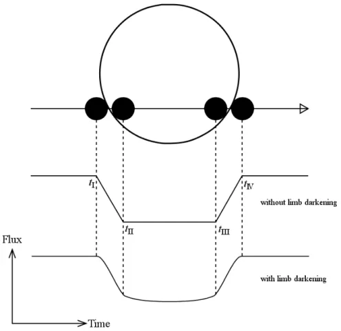
1.1 Illustration of a transit and the corresponding time-variation
of a stellar flux. . . 17
1.2 Example of grazing transit light curves. . . 19
1.3 Relations between orbital period and planetary mass of known exoplanets. . . 22
1.4 Relations between semi-major axis and orbital eccentricity of known exoplanets. . . 23
1.5 Relations between semi-major axis and spin-orbit misalign- ment of known transiting planets. . . 24
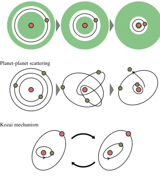
1.6 Illustrations of planetary migration processes. . . 26
2.1 Example of a linearity test frame in g′2-band. . . 33
2.2 Example of a linearity test result. . . 34
2.3 The light curves and the best-fit transit models of CVSO 30 observed by g2′-, r′2-, and zs,2-bands. . . 39
2.4 Top panel: The best-fit parameter and uncertainty of Rp/Rs in g′2-, r′2-, and zs,2-band from Table 2.1. Bottom panel: The wavelength dependence of Rp/Rs at the impact parameter fixed by b = {0.97, 1.05, 1.18} . . . 40
3.1 The light curves and the best-fit transit models of CVSO 30. 48 3.2 Continuation of Figure 3.1. . . 49
3.3 Continuation of Figure 3.2. . . 50
3.4 Continuation of Figure 3.3. . . 51
3.5 Continuation of Figure 3.4. . . 52
3.6 Continuation of Figure 3.5. . . 53
3.7 Continuation of Figure 3.6. . . 54
3.8 Continuation of Figure 3.7. . . 55
3.9 Continuation of Figure 3.8. . . 56
3.10 Continuation of Figure 3.9. . . 57
3.11 Time evolution of fitted Rp/Rs. . . 58
3.12 Time evolution of fitted b. . . 59
4.1 Model light curve including gravity-darkening effect. . . 63 11
4.2 Residual between the observed and calculated time of transit center. . . 66 4.3 Time evolution of the orbital inclination. . . 67 4.4 Periodogram showing time variations of the orbital inclination. 68 4.5 Relations between Rp/Rs and fading duration . . . 69 4.6 Illustrations showing the candidates of the origin of fading
events proposed by Yu et al. (2015). . . 72 4.7 Illustrations based on our result. A dust clump eclipses the
host star. . . 72
List of Tables
2.1 Best-fit parameters and the uncertainties . . . 38
2.2 Rp/Rs and the uncertainties in case of various fixed impact parameters for each band . . . 38
3.1 Summary of the observations . . . 42
3.2 Best-fit parameters and uncertainties . . . 44
3.3 Continuation of table 3.2. . . 45
3.4 Continuation of table 3.3. . . 46
3.5 Continuation of table 3.4. . . 47
4.1 Comparison between the observed depth and the gravity- darkened transit model depth . . . 63
4.2 Best-fit parameter for fading period. . . 66
4.3 Comparison between the results of this work and the fading origin candidate from Yu et al. (2015). . . 72
13
Introduction
In this chapter, we introduce the observational and theoretical background of studies on exoplanets.
1.1 Exoplanet
A couple of decades have passed since the first discovery of an exoplanet by Mayor & Queloz (1995). The first detected exoplanet 51 Pegasi b is a gas giant orbiting close-in around a Sun-like star. Hence, this planet has a high equilibrium temperature above 1300 K (Mayor & Queloz, 1995) and is called a “Hot Jupiter.” Hot Jupiters are considered to have migrated from outer orbits because they are unable to form in situ but rather must have formed in an outer orbit. We introduce planetary formation in Section 1.1.2 and orbital evolution in 1.1.3.
Most exoplanets are very faint and have large contrasts with their host stars; therefore, indirect methods are often used for observing exoplanets. For example, the radial-velocity method, which enabled the first detection of an exoplanet is a method based on measurement of the radial velocity of the stellar motion by the planetary gravitation. This method is sensitive to close-in and massive planets. However, the radial velocities of active and fast rotating stars are difficult to measure. As another example, the microlensing method is a technique that uses brightening by gravitational microlensing, which occurs when a foreground star happens to pass very closely to the line of sight of a background star. If the foreground star has planetary companions, the light curve varies depending on the mass of planet or the separation. This method is able to find planets of several Earth masses. However, follow-up observations are impossible because microlensing is a one-time event.
The transit method is useful when a planet passes across the face of its host star. This method has an advantage of obtaining a planetary radius with a close-in orbit. Since this thesis is mainly based on transit observa-
15
tions, in Section 1.1.1, we present a detailed description of transit observa- tions.
1.1.1 Transit Observation
When a planetary orbital plane from an observer is ∼ 90◦ from an observer (edge-on), a host star is occulted by the planet (upper light curve of Figure 1.1). Then, the observer can detect a flux fading; this is called the transit method. The first transit detection was an observation of HD 209458b by Charbonneau et al. (2000) and Henry et al. (2000). Transiting planets are discovered by follow-up observations of planets that are detected by the radial-velocity method in addition to ground or space surveys (e.g. HAT: Bakos et al. (2002); WASP: Pollacco et al. (2006); CoRoT: Baglin et al. (2002); Kepler: Borucki et al. (2003)).
To observe transits, we need to calculate the transit timing. A time of transit center Tc is
Tc= nP + T0 (1.1)
where n is an integer, P is an orbital period, and T0 is a reference time of transit center.
In a non-grazing transit, there are four contacts between the stellar and planetary disks (tI–tIV) in Figure 1.1. The total duration is Ttot = tIV− tI, the full duration is Tfull = tIII− tII, the ingress duration is τing= tII− tI, and the egress duration is τegr= tIV− tIII. The duration is calculated using the orbital parameters,
tIII− tII= P 2π!1 − e2
" fIII fII
# r(f ) a
$2
df (1.2)
where e is the orbital eccentricity, r is the distance from the host star to the planet, f is the orbital phase, and a is the orbital semi-major axis. For a circular orbit, the durations are written as
Ttot ≡ tIV− tI=
P π sin
−1
%Rs
a
!(1 + Rp/Rs)2− b2 sin i
&
(1.3)
Tfull≡ tIII− tII= P π sin
−1
%Rs
a
!(1 − Rp/Rs)2− b2 sin i
&
(1.4)
where Rs is the stellar radius, Rp is the planetary radius, i is the orbital inclination, and b is the impact parameter, which is
b = a cos i Rs
' 1 − e2 1 + e sin ω
(
(1.5)
Figure 1.1: Illustration of a transit and the corresponding time-variation of a stellar flux. tI, tII, tIII, and tIV are the first, second, third, and fourth contacts, respectively. The ingress and egress durations are tI–tIIand tIII–tIV, respectively.
The total flux of the star and planet F (t) is expressed as F (t) = Fs(t) + Fp(t) −' Rp
Rs
(2
αFs(t) (1.6)
where Fs(t) is the stellar flux, Fp(t) is the planetary flux, and α is a dimen- sionless function of the overlap area between the stellar and planetary disks. Generally, Fs(t) varies owing to flares, starspots, plages, tidal deformation, and so on; however, Fs(t) is taken here to be constant for simplicity. Now, we only have to consider f (t) ≡ F (t)/Fs, that is
f (t) = 1 +' Rp Rs
(2
Ip(t) Is −
' Rp
Rs (2
α (1.7)
where Ip and Is are the planetary and stellar intensities, respectively. Ip
varies in time according to the planetary phase function and the planetary atmospheric variations. Ip may be considered constant in the time scale of one transit; therefore, only α varies in time and can be approximated by a trapezoid. Then, the transit depth δ is written as
δ ≈' RRp
s
(2#
1 −IpI(t)
s
$
(1.8) For negligible intensity from the planetary night side,
δ ≈' RRp
s
(2
(1.9) If the variation of flux is approximated by a trapezoid, the light curve of ingress and egress are linear functions of time; however, this does not actually occur because of the nonuniform planetary motion. Hence, the occultation area is not a linear function (Mandel & Agol, 2002).
Additionally, the transit bottom is not flat because of the nonuniform stellar disk intensity. The stellar disk is bright at its center and faint in the outer regions, which is called “limb darkening.” For this reason, the transit is deeper when the planet is at the center of stellar disk, and shallower when the planet is in the stellar limb. Limb darkening is caused by differences in the temperature and altitude in the stellar atmosphere. The intensity profile I(X, Y ) with the sky in the X–Y plane is
I ∝ 1 − u1(1 − µ) − u2(1 − µ)2 (1.10) where µ ≡ √1 − X2− Y2 and {u1, u2} is the limb darkening coefficient, which is calculated by a stellar atmosphere model or is obtained from a transit light curve. A light curve including limb darkening is shown at the bottom of Figure 1.1.
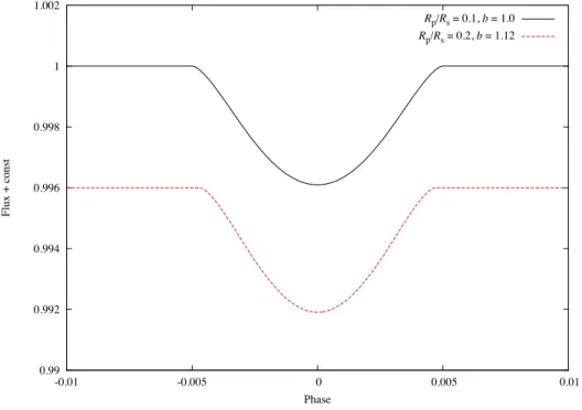
In case of a grazing orbit, tIIand tIIIdisappear. Hence, the transit bottom becomes V-shaped or round-bottom. Additionally, Rp/Rs and b are degen- erate when the transit path grazes the stellar disk. For example, the transit light curve with Rp/Rs= 0.1, b = 1.0 and that with Rp/Rs = 0.2, b = 1.12 have approximately the same shape (Figure 1.2). These degeneracies cause large errors in Rp/Rs and b.
1.1.2 Planetary Formation
Planetary formation theories have evolved from theories of the formation of the solar system. Safronov (1972) and Hayashi, Nakazawa, & Nakagawa (1985) constructed the solar system formation model using a ∼ 0.011 M! protoplanetary disk. These are the origins of core accretion models (e.g. Kokubo & Ida, 2002).
In a core accretion model, dust grains in the protoplanetary disk drop onto the equatorial plane and merge into planetesimals. Planetesimals merge mutually and grow into protoplanets. In the first stage of the planetesi- mals growth, the process of increasing mass is the runaway growth mode (e.g. Tanaka & Nakazawa, 1994). The mass increasing rates of planetesimals are faster in the massive planetesimals in the run- away growth mode. The protoplanets grown in this manner scat- ter other planetesimals and the growing rates slow down (Kokubo
& Ida, 1998). This stage is known as the oligarchic growth mode. When protoplanets grow to be ∼ 10M⊕ (Mizuno, 1980; Ikoma, Nakazawa, & Emori, 2000), gas accretion onto the protoplanet starts runaway growth (Bodenheimer & Pollack, 1986; Pollack et al., 1996). The accreted planet continues to grow until gas around the planet disappears. Note that the formation time of the core is pro- portional to the cube of the radius from the central star. Therefore, gas giants do not form in regions too distant from the central star, because the disk gas has dissipated in the time the core has formed. The lifetime of protoplanetary disks is 106–107 yr according to the observations of T-Tauri stars in young clusters (Beckwith et al., 1990; Haisch, Lada, & Lada, 2001; Hern´andez et al., 2007). Gas giant formation is completed by the lifetime of protoplanetary disks. However, there are several problems: infall of dust into the host star before the for- mation of planetesimals by gas drag (e.g. Brauer, Dullemond, & Henning, 2008), destruction of kilometer-scale planetesimals by mutual collision (e.g. Ida, Guillot, & Morbidelli, 2008), and infall of the planet into the host star by gravitational interaction with the protoplanetary disk.
In contrast, Cameron (1978) argued that planets form in the ∼ 1 M! protoplanetary disk with gravitational instability of the disk. In the gravita- tional instability model, giant planets form by the collapse of the protoplan- etary disk. The biggest advantage of the gravitational instability model over
0.99 0.992 0.994 0.996 0.998 1 1.002
-0.01 -0.005 0 0.005 0.01
Flux + const
Phase
Rp/Rs = 0.1, b = 1.0 Rp/Rs = 0.2, b = 1.12
Figure 1.2: Example of grazing transit light curves. The solid black line shows the transit with Rp/Rs= 0.1, b = 1.0. The dashed red line shows the transit with Rp/Rs= 0.2, b = 1.12. These very similar transit shapes cause degeneracy of the fitted parameters Rp/Rs and b.
the core accretion model is the ability to neglect the above problems because the gas giant forms directly from the protoplanetary disk. This model also has problems; an abundance of the planets is consistent with one of host star and rocky planets do not form by gravitational instability. However, some of answers for these problems have been proposed recently (e.g. Nayakshin, Helled, & Boley, 2014). Additionally, occurrence rates of gas giants increase with host star metallicity (e.g. Wang & Fischer, 2015). The core accretion model can explain it, but the gravitational in- stability model cannot. Therefore, core accretion has been considered the
“standard” model in planet formation. 1.1.3 Orbital Evolution
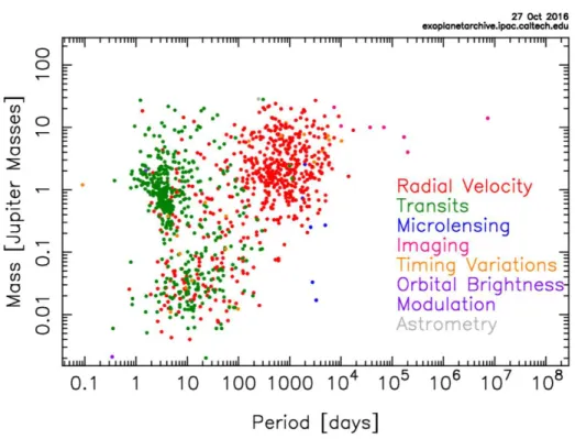
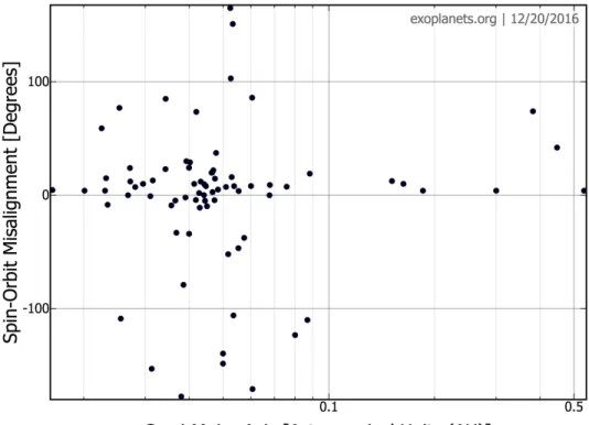
Planetary orbits of exoplanets are known to show a much wider distribu- tion than those of the solar system. Figure 1.3 shows known exoplanets’ relations between orbital period and planetary mass. The group of Jupiter- mass planets with an orbital period less than ∼ 10 days is known as hot Jupiters. Additionally, certain exoplanets have highly eccentric orbits (Fig- ure 1.4) and/or spin-orbit misalignment (Figure 1.5). Note that spin-orbit misalignment can only be measured for only transiting planets. Hence, the planets for which spin-orbit misalignment has been measured only have only close-in orbits.
As shown in the figures, many planets including hot Jupiters exist within the orbits of solar system planets. This section describes theories regarding how these planets have these strange orbits.
Whether planets form by core accretion or gravitational instability, gas giants with small orbits (close-in planets), such as hot Jupiters, cannot form in situ. Hence, there is a mechanism for planetary migration from an outer orbit to an inner orbit.
The planet interacts with the gaseous disk and receives the angular mo- mentum from the gas in the inner orbit and gives the angular momentum to the gas in the outer orbit. In general, the torque passed from the planet to the outer orbit is larger; hence, the planet migrates to the inner orbit in an isothermal gas disk (Ward, 1986). This mech- anism is called “Type I migration,” which is accentuated in rocky planets so as not to influence the density distribution of a disk. If the planet grows to dozens of Jupiter masses, the planet opens the gap in the disk. Then, the planet is fixed to the gap by gravitational interaction and migrates to the inner orbit (Lin & Papaloizou, 1985), as shown in the upper panel of Figure 1.6. This mechanism is called “Type II migration.” The planets fall in while maintaining circular orbits in Type I and Type II migrations.
On the other hand, gravitational perturbations from other objects also cause planets to shift their orbits. In the case of planet–planet scattering, planetary orbits shift or release from a planetary system when three or more
Figure 1.3: Relations between semi-major axis and planetary mass of known exoplanets as of October 2016. The data of exoplanets are from http://exoplanetarchive.ipac.caltech.edu. The colors of points indicate de- tection methods.
Figure 1.4: Relations between semi-major axis and orbital eccentricity of known exoplanets as of December 2016. The data of exoplanets are from http://exoplanets.org.
Figure 1.5: Relations between semi-major axis and spin-orbit misalignment of known transiting planets as of December 2016. The data of exoplanets are from http://exoplanets.org.
gas giants exist in the planetary system (e.g. Marzari & Weidenschilling, 2002), as shown in the middle panel of Figure 1.6. Then the orbit of the remaining planet is deformed into an eccentric orbit. In the wide binary sys- tem, the planetary orbit is perturbed from a stellar companion by the Kozai mechanism (Kozai, 1962). The Kozai mechanism oscillates the eccentricity and orbital inclination of the planetary orbit, as shown in the bottom panel of Figure 1.6. The existence of eccentric planets and misalignment planets is a testament to planet–planet scattering and/or the Kozai mechanism.
If a planet with a highly eccentric orbit gets close enough to exert tidal force, the planetary semi-major axis decreases by tidal dissipation from the host star. Thus, the planetary orbit becomes a circular close-in orbit, such as that of a hot Jupiter. Therefore, there is no way to the know orbital migration mechanisms of hot Jupiters, excepting young planets before tidal circularization. According to Ivanov & Papaloizou (2004), the tidal circu- larization timescale is greater than a few gigayears for a planet with mass of the order of the Jupiter mass and final period ∼ 1–4.5 days. Hence, we must observe young planets to inspect the mechanism of orbital migration. As described above, there are several mechanisms of the hot Jupiters’ orbital evolution. Knutson et al. (2014) searched for distant massive com- panions to known hot Jupiters that may have influenced the dynamical evolution of the planetary systems. They estimated that 51 ± 10% of the hot Jupiters have a companion with orbital semi-major axes in the range of 1–20 AU and masses in the range of 1–13 MJup, while the masses of the planetary companion tend to be comparable to or larger than the transiting hot Jupiters. They found no statistically significant difference between the frequency of companions to transiting planets with misaligned or eccentric orbits and those with well-aligned, circular orbits.
Simpson et al. (2011) find that the host stars have Teff < 6250 K and conform to the trend of cooler stars having low obliqui- ties. This is suggests that the tidal torques experienced by cooler stars, with larger convective zones, could cause their envelopes to quickly align with a planetary orbit, thereby erasing any initial misalignment.
1.2 Observational Studies for Young Giant Plan-
ets
Giant planets undergoing formation or shortly after formation can be mainly observed by direct imaging (e.g. Marois et al., 2008; Kuzuhara et al., 2011). These planets are all gas giants with large semi-major axes, and hence, again, their formation cannot be explained by core accretion, because of their young ages compared to the giant planet forming time predicted by the core accretion model. The gravitational instability model can explain
Figure 1.6: Illustrations of planetary migration processes. Top: Type II migration. Middle: Planet–planet scattering. Bottom: Kozai mechanism.
the formation of these planets; however, it is unknown how many planets form by gravitational instability. Therefore, although the important point is discovering planets with smaller semi-major axes, the direct imaging can- not observe within the region of several AU with the current technology. Furthermore, neither the radii nor masses of the planets observed by direct imaging are directly derived, owing to their dependence on the planetary formation and evolution model.
For the radial-velocity method, some planet candidates have been recently found. Donati et al. (2016) discovered a hot Jupiter candidate around a < 2 Myr weak-line T-Tauri star V830. As an- other example, Johns-Krull et al. (2016) found out a giant planet candidate around a ∼ 2 Myr classical T-Tauri star CI Tau by the radial-velocity method. The masses of these planet candidates detected by radial-velocity method are able to be measured; how- ever, their radii cannot be measured. By contrast, the transit method is able to measure planetary radii and then obtain the densities by the com- bination with the radial-velocity method. It is noted that the transit method is sensitive to the nearby host star; therefore, it is complementary to direct imaging.
As described in Section 1.1.3, observations of young hot Jupiters are needed to understand the process of orbital migration. However, such young transiting planets have only very rarely yet been found. Although the origin is not a planet, Rodriguez et al. (2017) found dimming events of the weak-line T-Tauri star V1334. The possible origin is an orbiting body (e.g. a disk warp or dust trap), enhanced disk winds, hydrodynamical fluctuations of the inner disk, or a significant increase in the magnetic field flux at the surface of the star. One of the few examples of a young planet candidate was reported recently using the transit method (van Eyken et al., 2012). Thus, we will explain this source in detail.
1.3 Previous Studies for CVSO 30
CVSO 30b (PTFO 8-8695b) is a candidate transiting hot Jupiter around a weak-line T-Tauri star in the Orion OB1a/25-Ori region found by van Eyken et al. (2012). The age of CVSO 30 is estimated as ∼ 3 Myr (Brice˜no et al., 2005), which makes this object the youngest candidate planet. The host star is an M3 type pre-main-sequence star in the Orion OB1a region at a distance of 323+233−96 pc. CVSO 30 has a mass of 0.44 M! (using the Baraffe et al. (1998) model) or 0.34 M!(using the Siess, Dufour, & Forestini (2000) model), a radius of 1.39 R!, and an effective temperature of 3470 K (Brice˜no et al., 2005). The candidate planet has an orbital period of 0.448413 ± 0.000040 days, which is comparable to the rotational period of
the host star, a mass of Mp≤ 5.5 ± 1.4 MJup, a radius of 1.91 ± 0.21 RJ up, and an orbital semi-major axis of 0.00838 ± 0.00072 AU (van Eyken et al., 2012).
In contrast to other planetary transiting objects, the observed fading light curves of CVSO 30 change with the observational epoch. Barnes et al. (2013) explained this by a combination of the precession of the ascending node of planetary orbit and the stellar gravity-darkening effect, assuming synchronization of the stellar rotation and planetary orbital motion. Kami- aka et al. (2015) added the photometric data and reanalyzed the light curves using precession and the gravity-darkening model without the co-rotation. Examples of nodal precession had been found in Kepler-13b (Szab´o et al., 2012) and WASP-33b (Johnson et al., 2015). Schmidt et al. (2016) discovered an additional planet CVSO 30c in the outer or- bit (P ∼ 27000 yr) by the direct imaging method. The best-fitted planetary mass of 4–5 MJup suggests that the CVSO 30 planetary system has experienced the planet–planet scattering events.
On the other hand, Ciardi et al. (2015) observed a primary transit at 4.5 µm using Spitzer IRAC without any sign of a secondary eclipse. In addi- tion, their radial-velocity measurement showed no evidence of the Rossiter– McLaughlin effect. Yu et al. (2015) observed 13 events with the i′-band and 13 other events with the I + z-band over three years. They found that the fading period is not constant. Multiband simultaneous observations were performed for five fading events, of which r′- and I + z-bands were observed simultaneously on two nights, i′- and g′-bands were observed on another two nights, and I +z- and H-bands were observed on one night. Their multiband observations showed that the depths of all but one fading event were deeper at short wavelengths, while one of the fading events showed the same depth in the r′- and I + z-bands showed the same depth.
In addition, they tried to detect the secondary eclipse at infrared and the Rossiter–McLaughlin effect by high-resolution spectroscopy. They could not find an expected signature in either observation but found strong variable Hα and Ca H and K lines. Hence, Yu et al. (2015) argued that the transit-like events were unlikely to be caused by a giant planet, but rather caused either by starspots near the rotational pole, circumstellar dust clump transit, or occultation of an accretion hotspot. Raetz et al. (2016) observed 33 fading events and found that the period of the fading event was shortened. They also observed a fading event in the B- and R-bands simultaneously, and found that the light curve showed the same depth. Johns-Krull et al. (2016) observed excess Hα emission from CVSO 30. The excess Hα emission was not detected constantly; however, the observed velocity motion in transit was almost as expected. They argued that this excess came from the planet in the middle of mass loss.
1.4 Our Motivation
Our motivations in this thesis are to investigate what is happening around the critical candidate(s) of young transiting planet. It is important to study the scene of planetary formation; however, few observational studies have been carried out, except for on CVSO 30. Hence, CVSO 30 is currently the most important object for understanding the environment around a young star.
As presented above, the studies of wavelength dependence using multi- band simultaneous photometry by Yu et al. (2015) and Raetz et al. (2016) are inconsistent. However, CVSO 30 has a large stellar variability and its fading shape changes with time. Therefore, simultaneous observations are required for measuring the wavelength dependence of fading events. It has been difficult to discern the trend of wavelength dependence from previous studies, because they have all been performed using only by two colors.
In this paper we report our results of independent three-band simul- taneous transit photometry for a fading event of CVSO 30. We use the Multicolor Simultaneous Camera for studying Atmospheres of Transit- ing exoplanets (MuSCAT) (Narita et al., 2015) on the 188-cm telescope at Okayama Astrophysical Observatory (OAO) to investigate the wavelength dependence of a fading event. The multiband simultaneous obser- vations realize a comparison between wavelength dependence of fading depth and possible origins such as planetary atmosphere and dust cloud. Additionally, we observe the fading events over three years in a near-infrared wavelength for the first time. As a result, we find double fading events for the first time. The infrared long- term observations enable the discussion of the time-evolution of Rp/Rs, the impact parameter, and the fading duration with re- duced baseline variations. Stellar variation of CVSO 30 occurs mainly by starspots. An advantage of infrared observations over optical observations is their robustness for starspots, which are different in temperature.
I contributed to observations and discussions and so on. I also developed the MuSCAT instrument as a member of the MuSCAT team. The long-term observations were primarilly performed by my proposal for the thesis-supporting program in OAO. I had a key role in the discussions with colleagues.
We describe the multiband simultaneous observations for CVSO 30, anal- ysis, and results in Chapter 2. Chapter 3 shows the results of long-term observations. In Chapter 4, we discuss the origin of transit-like events based on the results of both Chapters 2 and 3. Finally, we summarize our results and future plans in Chapter 5.
Multiband Simultaneous
Observations for CVSO 30
(Based on a paper by Onitsuka et al., accepted for PASJ)
As described in Section 1.3, the origin of fading events of CVSO 30 is yet unidentified. We performed the first simultaneous three-color photometry of CVSO 30 to investigate the origin of fading events. In this chapter, we describe in detail the multicolor simultaneous observations, analysis and results. The discussion is presented in Chapter 4, based on the combined results of this and the next chapters. My contribution to the development of the instrument (MuSCAT) is also described here.
2.1 Observations
2.1.1 The Multicolor Simultaneous Camera for studying At- mospheres of Transiting exoplanets (MuSCAT)
The Okayama Astrophysical Observatory (OAO) 188-cm telescope is one of the largest telescopes in Japan. The OAO 188-cm telescope is an equatorial optical telescope. The pointing accuracy is approximately 10 arcsec.
We developed the Multicolor Simultaneous Camera for studying Atmo- spheres of Transiting exoplanets (MuSCAT) (Narita et al., 2015) on the OAO 188-cm telescope for simultaneously taking optical imaging data with three colors. MuSCAT has three 1024 × 1024 pixel CCDs and two dichroic mirrors for simultaneous observation. The field of view is 6.1 × 6.1 arcmin2 with a pixel scale of 0.358 arcsec/pixel. Filters for the g2′ (400–550 nm), r2′ (550–700 nm), and zs,2 (820–920 nm) bands are simultaneously avail- able using Astrodon Photometrics Generation 2 Sloan filters. The principal purpose of MuSCAT is to perform high-precision multicolor transit photom- etry. For this purpose, MuSCAT has a capability of self-autoguiding, which enables it to fix positions of stellar images within ∼ 1 pixel.
31
I have contributed to the measurement of CCD specifications. I tested the linearity of MuSCAT CCDs for each readout speed and each gain. I will explain this test in detail here.
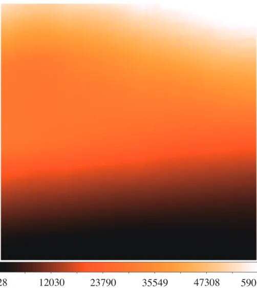
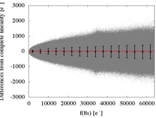
My method is based on a previous study of the CCDs on the High Dis- persion Spectrograph (HDS) of the Subaru telescope (Tajitsu et al., 2010). First, I construct linearity test frames with gradational counts on the CCDs, by opening only a half of the tertiary mirror cover and inserting a black plate into the light path in front of MuSCAT. Figure 2.1 shows an example of a linearity test frame. Second, I monitor counts of the filament lamp until the filament lamp is stabilized. I note that it takes approximately two hours until the counts become nearly constant. I then start linearity test expo- sures as follows. I first determine an exposure time for each CCD, which provides counts from the bias level to saturation level gradationally on the CCDs. I define the frames with the above exposure time as “A” frames and those with one half of the exposure time as “B” frames. I then consider A and B frames alternately until obtaining 20 of each frames type. I have repeated such exposures for each gain and each readout speed, i.e., for the gain modes of 1, 2, 4 e−/ADU, and for the readout speeds of 100 kHz and 2 MHz. Subsequently, I subtract a median bias frame for each gain and each readout speed. I then make a new frame that computes photon counts of each pixel in an A frame minus twice the photon counts for the same pixel in a B frame using adjacent A and B frames (39 pairs in total for each gain and each readout speed). I define those frames as “C” frames (namely, C = A − 2 × B for each pixel). To visualize the linearity of the CCDs, I plot electron counts (namely, photon counts × gain) of corresponding pixels in A and C frames on X- and Y-axis respectively. An example of such a plot is shown in Figure 2.2. I finally fit the plotted data with a linear function (Y = aX) using the data up to X = 64000, and the best-fit linearity slopes are summarized in Table 2.1.1. Based on the above test, I have confirmed that MuSCAT CCDs have a good linearity within ∼ 0.21% at a maximum up to the saturation level. These results indicate that the effect of nonlin- earity is well negligible, even for high-precision transit photometry if the counts of stars do not change drastically during observations. If necessary, I will use these data for nonlinearity corrections.
2.1.2 Transit Observations
We observed a fading event of CVSO 30 on 2016 Feb 9 (UT). We used the MuSCAT on the 188-cm telescope at OAO.
For precise differential photometry, dithering observations cause system- atic error because of the incomplete correction of the flat pattern. For this reason, we fix the stellar position on the CCD using the self-autoguiding soft- ware (Narita et al., 2015). This software detects the stellar barycenter on science frames, and then the software corrects the attitude of the telescope
328 12030 23790 35549 47308 59010
Figure 2.1: Example of a linearity test frame in g′2-band. Counts of the dark region are nearly at the bias level and those in the brightest region are saturated.
Gain mode ADC speed [Hz] g′2-band r′2-band zs-band linearity slope [%] linearity slope [%] linearity slope [%] 1 2 × 10⁶ 0.154 ± 0.062 0.104 ± 0.051 0.204 ± 0.026
1 × 10⁵ −0.198 ± 0.071 −0.055 ± 0.043 −0.133 ± 0.040 2 2 × 10⁶ 0.016 ± 0.072 0.018 ± 0.045 0.112 ± 0.025
1 × 10⁵ −0.210 ± 0.069 0.005 ± 0.043 −0.061 ± 0.039 4 2 × 10⁶ 0.169 ± 0.044 0.120 ± 0.037 0.115 ± 0.030
1 × 10⁵ −0.059 ± 0.077 −0.085 ± 0.043 −0.037 ± 0.034
Figure 2.2: Example of a linearity test result. The horizontal axis (f(8s) [e−]) indicates electron counts in 8 seconds. The vertical axis shows the flux ratio parameter which is defined as f(8s) - 2 × f(4s) [e−].
to maintain the stellar position on the CCD. Additionally, it is important to maximize the received stellar photons for precise photometry. However, several pixels are saturated in less exposure time in focus. Therefore, we defocus stellar images to torus PSF for many pixels to be able to receive more photons.
The exposure times were 60 seconds for all the bands. We obtained 172, 221, and 220 frames for the g2′-, r′2-, and zs,2-bands, respectively, in 4.4 hours.
2.2 Data Reduction and Aperture Photometry
Our data reduction and aperture photometry method used the customized pipeline by Fukui et al. (2011). Firstly, we make the bad pixel mask using a merged flat image. We define outliers with greater than 3σ in merged flat images as bad pixels. The values of the bad pixels are replaced with zero. Secondly, we subtract the merged dark image from the flat images and mask the bad pixels. The masked flat images are merged after being normalized. Finally, we subtract the merged dark image from the science frames and divide the science frames by the merged flat image.
In aperture photometry, we firstly detect the stellar barycenter on each frame. Then we obtain the shifts of the stellar position on the detector be- tween each pair of consecutive images. Next, we photometer the target and the comparison star in the aperture radius centered on the stellar barycen- ter. We also measure the sky background by the torus region centered on the stellar barycenter. We calculate target and comparison flux by subtracting the sky background flux from the stellar flux. Finally, we obtain the relative flux by dividing the target flux by the comparison flux.
2.2.1 Light Curve Fitting
Our analysis method follows the method of Fukui et al. (2016). First, we make light curves using different combinations of comparison stars and var- ious aperture radii. We choose comparison stars that are neither saturated nor variable stars and the aperture radius that produces a light curve with minimum dispersion outside the fading event. The selected aperture radii are 17, 14, and 12 pixels for the g′2-, r′2-, and zs,2-bands, respectively, and the comparison stars are the same two stars for each band. Second, we convert the time system of Modified Julian Day (MJD) in Universal Time Coordi- nate (UTC), which is recorded in the FITS headers into Barycentric Julian Day (BJD) in Barycentric Dynamical Time (TDB) using the algorithm of Eastman, Siverd, & Gaudi (2010). The produced light curves are shown in the top panels in Figure 2.3.
Next, we fit the light curves with a transit model, assuming that the fading event is caused by a transiting spherical body. We use the transit
light curve model by Ohta, Taruya, & Suto (2009) which is comparable to the quadratic limb-darkening law case of Mandel & Agol (2002). The transit modeling parameters are the time of the transit center Tc, the ratio of the planetary-to-stellar radii Rp/Rs, the ratio of the semi-major axis to the stellar radius a/Rs, and the impact parameter b. The variations seen outside the fading event seem to be caused by the variability of CVSO 30 itself or comparison stars, with changing of air mass, shifting of stellar images on the detector and so on. We fit the transit light curves and baseline model at the same time using customized code by Fukui et al. (2016), which is based on Narita et al. (2007) and Narita et al. (2013). A transit and out-of-transit (OOT) model is given by
F = (k0+)
i=1
kiXi) × Ftr (2.1)
where F is the relative flux, Ftr is the transit light curve model, {X} are time-dependent observed variables such as, for example, air mass, shifts of stellar position on the CCD, and so on, and {k} are coefficients (Fukui et al., 2016).
We fix the orbital eccentricity to zero and the limb-darkening param- eters to the values from Claret, Hauschildt, & Witte (2012), {u1, u2} = {0.8067, 0.0861}, {0.8423, −0.0160}, {0.2946, 0.3569} for the g2′-, r
′
2-, and zs,2
bands, respectively. In addition, we put a Gaussian prior for a/Rs = 1.685 ± 0.064, based on the value obtained by van Eyken et al. (2012).
To choose the most appropriate combination of free parameters, we opti- mize the parameters using the AMOEBA algorithm (Press et al., 1992) and evaluate the Bayesian Information Criterion (BIC: Schwarz (1978)). The BIC value is defined by BIC ≡ χ2+ klnN , where k is the number of free parameters and N is the number of data points. We calculate the BIC val- ues for each light curve and parameter, then we pick out the combinations with the minimum BIC value for each band. For {X}, we test different combinations of the time t, the square of time t2, the airmass z, and the relative stellar positions on the CCD ∆x and ∆y. Based on the minimum BIC, we adopt k0, kt for all bands.
To take into account the time-correlated noise (so-called red noise; e.g. Pont, Zucker, & Queloz (2006); Winn et al. (2008)), we multiply each flux uncertainty by the red-noise factor β which is the ratio of the observed stan- dard deviation of the binned light curve to the expected standard deviation of the unbinned and non-time-correlated light curve. The binning sizes are between 5 and 20 minutes. We obtain the median of β for each binning size and multiply the median β by the uncertainty of each dataset. The typical photometric errors including β are 2.1%, 0.87%, and 0.54% for the g′2-, r′2-, and zs,2-bands, respectively.
After that, to estimate the uncertainty of the free parameters, we analyze the chosen light curve by the Markov Chain Monte Carlo (MCMC) method
following Narita et al. (2013) and Fukui et al. (2016). We first independently analyze the light curves for each band, and after that we jointly analyze all the light curves. We calculate a MCMC chain with 107 steps and the first 106 steps are excluded as burn-in. We define 1σ uncertainties as the range of the parameters between 15.87% and 84.13% of the merged posterior distributions.
2.3 Results
Table 2.1 shows the best-fit transit parameters and uncertainties obtained by the MCMC analysis. Note that we obtain consistent results when we fit the light curves that are produced by different baseline models with comparable BIC values. We show the transit light curves and the best-fit models of each observation in Figure 2.3.
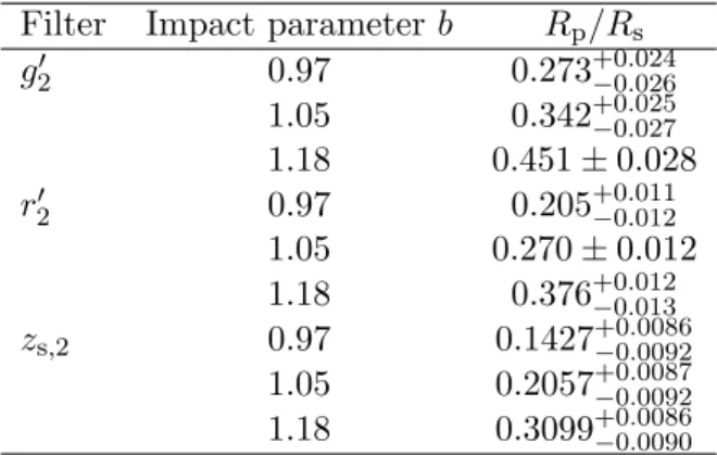
van Eyken et al. (2012) and Yu et al. (2015) reported that the transit depth of CVSO 30 changes with the observational epoch. According to Yu et al. (2015), the loss of light was 20–30% larger in the bluer band on 2012 Dec 14 at r′- and I + z-band, on 2014 Jan 9 and 2014 Jan 18 at i′- and g′-band, and on 2014 Jan 19 at I + z- and H-band, respectively. How- ever, the loss of light in r′ was essentially the same as in I + z on 2012 Dec 15. We present the transit depth in g′2-, r′2-, and zs,2-bands observed simultaneously. Figure 2.4 gives the wavelength dependence of Rp/Rs. The top panel shows the best-fit parameters for Rp/Rs and their uncertainties for each band in Table 2.1. The uncertainties are influenced by the impact parameter b which is grazing. We recalculate the Rp/Rsand their uncertain- ties fixing the impact parameter at the median and 1 σ upper/lower limit b = {0.97, 1.05, 1.18} to highlight the wavelength dependence of Rp/Rs(Fig- ure 2.4: bottom panel; Table 2.2). As the result, we find that the wavelength dependence in Rp/Rs is apparent, regardless of the value of b.
Table 2.1: Best-fit parameters and the uncertainties Parameter Value Uncertainty Tc [BJDTDB] 2457428.0758 +0.0017−0.0014
a/Rs 1.730 ±0.061
b 1.054 +0.121−0.086
Rp/Rs (g′2) 0.344 +0.111−0.075 Rp/Rs (r2′) 0.271 +0.105−0.066 Rp/Rs (zs,2) 0.206 +0.104−0.064
k0 (g′2) 1.0103 +0.0055−0.00434 k0 (r2′) 1.0016 +0.0017−0.0014 k0 (zs,2) 0.99713 +0.00080−0.00074
kt (g2′) 0.010 +0.059−0.049 kt (r′2) 0.018 +0.019−0.017 kt (zs,2) −0.0489 +0.0093−0.0087
Table 2.2: Rp/Rs and the uncertainties in case of various fixed impact pa- rameters for each band
Filter Impact parameter b Rp/Rs
g′2 0.97 0.273+0.024−0.026 1.05 0.342+0.025−0.027
1.18 0.451 ± 0.028 r2′ 0.97 0.205+0.011−0.012
1.05 0.270 ± 0.012 1.18 0.376+0.012−0.013
zs,2 0.97 0.1427+0.0086−0.0092 1.05 0.2057+0.0087−0.0092 1.18 0.3099+0.0086−0.0090
0.94 0.96 0.98 1 1.02 1.04
Relative flux
g’2 r’2 zs2
0.94 0.96 0.98 1 1.02 1.04
Relative flux
g’2 r’2 zs2
-0.04 -0.02 0 0.02 0.04
-0.05 0 0.05 0.1
Residuals
BJD - 2457428
-0.05 0 0.05 0.1
BJD - 2457428
-0.05 0 0.05 0.1
BJD - 2457428
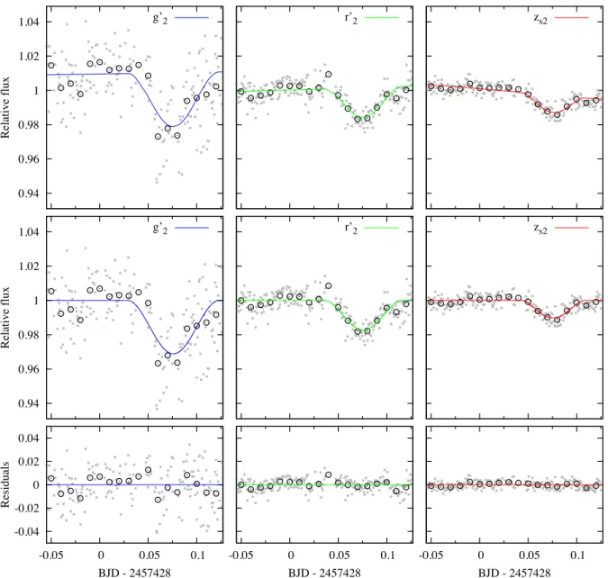
Figure 2.3: Top panels: Gray dots are the raw light curves of CVSO 30 observed by g2′-, r′2-, and zs,2-bands from the left. The black open circles are 0.01 days binned data. The solid lines are the best-fit transit models. Middle Panels: Light curves corrected by the baseline correction. Bottom panels: Residuals between the observed data and the best-fit model.
0.1 0.15 0.2 0.25 0.3 0.35 0.4 0.45 0.5
400 500 600 700 800 900 1000
Rp/Rs
Wavelength [nm]
0.1 0.15 0.2 0.25 0.3 0.35 0.4 0.45 0.5
400 500 600 700 800 900 1000
Rp/Rs
Wavelength [nm]
b = 0.97 b = 1.05 b = 1.18
Figure 2.4: Top panel: The best-fit parameter and uncertainty of Rp/Rs
in g′2-, r2′-, and zs,2-band from Table 2.1. Bottom panel: The wavelength dependence of Rp/Rsat the impact parameter fixed by b = {0.97, 1.05, 1.18}
Long-term Observations for
CVSO 30
CVSO 30 is reported to have light curve variations with observational epoch. To understand this, we need a long-term observation. Following the first si- multaneous three-color photometry of CVSO 30 to inspect the origin of fading events, we have conducted the first near-infrared long-term photom- etry of CVSO 30 over three years. In this chapter, we describe in detail the observations, analysis, and results. The discussion is presented in Chapter 4, based on the combined results of this and the previous chapters.
3.1 Observations
3.1.1 Instrument
The Okayama Astrophysical Observatory (OAO) 188-cm telescope and the Multicolor Simultaneous Camera for studying Atmospheres of Transiting exoplanets (MuSCAT) are described in Section 2.1.1.
The near-infrared imaging and spectroscopic instrument ISLE (Yanagi- sawa et al., 2006, 2008) on the Cassegrain focus of the OAO 188-cm telescope is an instrument for capturing near-infrared images or spectroscopic data. ISLE has a HAWAII 1k × 1k HgCdTe array and a 4.3 × 4.3 arcmin2 field of view. The pixel scale is 0.25 arcsec/pixel. The available filters are J-, H-, K-, Ks-, and some narrow-band filters.
3.1.2 Transit Observations
We observed 11 fading events of CVSO 30 with ISLE on OAO 188-cm tele- scope and one fading event with MuSCAT from 2012 to 2016. We used the J-band filter for ISLE observations and the g2′-, r′2-, and zs,2-bands simulta- neously for MuSCAT observations. The observation dates are summarized in Table 3.1.
41
Table 3.1: Summary of the observations
UT Date Instrument Filter No. of data points Exposure time [s]
2012 Nov. 27 ISLE J 342 60
2012 Dec. 1 ISLE J 178 60
2013 Dec. 2 ISLE J 107 120
2014 Jan. 24 ISLE J 91 120
2014 Feb. 10 ISLE J 99 120
2014 Feb. 19 ISLE J 95 120
2014 Nov. 18 ISLE J 77 120
2014 Nov. 22 ISLE J 188 120
2014 Dec. 5 ISLE J 140 120
2015 Jan. 10 ISLE J 153 120
2015 Dec. 1 ISLE J 205 120
2016 Feb. 9 MuSCAT g2′ 172 60
2016 Feb. 9 MuSCAT r′2 221 60
2016 Feb. 9 MuSCAT zs,2 220 60
To achieve high-precision photometry, we did not dither but fixed the target position on the detector, and defocused the stellar PSF (see Sec- tion 2.1.2). For the ISLE observations, we can use not only the self-autoguiding software but also the off-set autoguider. The self-autoguiding software is used in the observations after 2014 on both ISLE and MuSCAT.
3.2 Analysis
Our data reduction and aperture photometry method used the customized pipeline by Fukui et al. (2011), as described in Section 2.2. The light curve transit fitting method was also similar to Fukui et al. (2016), but we si- multaneously fit the 14 light curves. Barnes et al. (2013) pointed out the possibility of precession of the planetary orbit. When the planetary orbit precesses, the transit impact parameter varies because of the change in the orbital inclination. To consider the origin of fading events, we give an inde- pendent Rp/Rs and b for each light curve and a common a/Rs.
Some light curves observed in 2014–2015 exhibit “double fading,” which occurs after the first fading. In other words, there are two bottoms in one fading epoch. Therefore, we fit the light curves simultaneously for the first and second fading. When we fit the second fading, we mask the first fading by eye, and vice versa. Light curves with separated first and second fadings were observed on November 22, 2014, January 10, 2015, and December 1, 2015.
3.3 Results
Tables 3.2, 3.3, 3.4, and 3.5 show the best-fit transit parameters and uncer- tainties for the long-term observations obtained by the MCMC analysis. We show the transit light curves and the best-fit models of each observation in Figure 3.1, 3.2, 3.3, and 3.4.
As shown in the figures, the fading shapes of the light curves vary with observational epoch. This is a similar phenomenon to that reported by van Eyken et al. (2012), Yu et al. (2015) and Raetz et al. (2016). To solve the origin of shape changing, we give an independent Rp/Rs and b for each light curve. Additionally, we find “double fading” in one observational epoch on 2014 November 22 (JD 2456984), 2015 January 10 (JD 2457032), and 2015 December 1 (JD 2457358). Double fading events are previously unreported phenomena.
To understand these double fading events, we give the individual fitting parameters for the first and second fading events when double fading events are observed. For example, to fit the first fading event, we remove the data at the second fading in a visual way. We then fit the light curve without the second fading by the transit model. On the other hand, we employ the light curve without the data at first fading for to fit the second fading event. Accordingly, we obtain the two transiting parameter sets which are Tc, b, Rp/Rsand baseline correction factors for one double fading light curve. This assumption corresponds to two objects independently orbiting the host star. The variations of Rp/Rs and b are shown in Figures 3.11 and 3.12, re- spectively. These time variations include the degeneracy between Rp/Rs and b due to the obtained grazing orbit. Hence, these parameters have po- tentially more uncertainty than the best-fit parameters. However, either or both of Rp/Rs and b certainly exhibit large fluctuations. We will discuss these results for the long-term observations in the next chapter, combined with the results of Chapter 2.
Table 3.2: Best-fit parameters and uncertainties Common parameter Value Uncertainty
a/Rs 2.189 +0.025−0.025
Independent parameter
2012 Nov. 27 Value Uncertainty
Tc [BJDTDB− 2450000] 6259.14947 +0.00056−0.00050
b 0.722 +0.017−0.017
Rp/Rs 0.115 +0.002−0.002
duration [days] 0.0518 +0.0009−0.0008
k0 0.9127 +0.0023−0.0030
kt 0.2220 +0.0056−0.0056
kt2 -3.71 +0.06−0.07
kz 0.0797 +0.0025−0.0019
kx 0.0 (fixed)
ky 0.0 (fixed)
2012 Dec. 1 Value Uncertainty
Tc [BJDTDB− 2450000] 6263.17009 +0.00085−0.00084
b 0.888 +0.027−0.012
Rp/Rs 0.096 +0.006−0.004
duration [days] 0.0426 +0.0008−0.0007
k0 1.1086 +0.0033−0.0036
kt 0.1369 +0.0044−0.0047
kt2 0.0 (fixed)
kz -0.0848 +0.0027−0.0027
kx -0.00048 +0.00008−0.00012
ky 0.0 (fixed)
2013 Dec. 2 Value Uncertainty
Tc [BJDTDB− 2450000] 6629.07668 +0.00060−0.00051
b 1.056 +0.019−0.016
Rp/Rs 0.246 +0.015−0.013
duration [days] 0.0487 +0.0009−0.0008
k0 0.8959 +0.0016−0.0021
kt 0.5100 +0.0091−0.0136
kt2 -4.36 +0.11−0.09
kz 0.0701 +0.0012−0.0010
kx -0.00847 +0.00066−0.00073
ky 0.0 (fixed)