本文 総合研究大学院大学学術情報リポジトリ 甲1227 本文

Escape and Capture on Halo Orbit Manifolds using

Impulsive Maneuvers for Interplanetary Transfers:

Applications to an Interplanetary Transportation System

Masaki Nakamiya

Doctor of Philosophy

Department of Space and Astronautical Science, School of Physical Sciences,

The Graduate University for Advanced Studies, Japan

2008

ACKNOWLEDGMENTS

First of all, I would like to thank Prof. Makoto Yoshikawa of ISAS (Institute of Space and Astronautical Science) / JAXA (Japan Aerospace Exploration Agency), also affiliated with the Graduate University for Advanced Studies (Sokendai University), as one of my dissertation supervisors.

I would also like to express my appreciation to Prof. Hiroshi Yamakawa of Kyoto University, another supervisor of my dissertation, for providing advice and teaching.

I have gratitude to Prof. Daniel J. Scheeres of the University of Colorado at Boulder for welcoming me in the United States of America, and for providing valuable discussion and feedback about my research.

I would like to acknowledge my doctoral committee for giving comments and feedback on this work on this work.

I wish to express my thank to the Department of Space and Astronautical Science at the Graduate University for Advanced Studies (Sokendai University) for support of my research and my education, and would like to thank the members of Yoshikawa Lab seminar for helping me.

At last but not least, I thank my wife very much for her continuous support of my life.

ABSTRACT

Spacecraft escape and capture trajectories from/to Halo orbits of the L1 or L2 points using impulsive maneuvers at the periapsis of the manifolds for interplanetary transfers in the restricted Hill three-body problem were analyzed. This application is motivated by future proposals to place “deep space ports” at the Earth and Mars L1 or L2 points.

First, the feasibility of interplanetary trajectories between Earth Halo orbits and Mars Halo orbits was investigated, and such trajectories were designed with reasonable ∆V and flight time. Here, we utilized unstable and stable manifolds associated with the Halo orbits to approach the vicinity of the planet’s surface, and assumed impulsive maneuvers for escape and capture trajectories from/to Halo orbits. Thus, characteristics of periapsis of unstable and stable manifolds were investigated. It was found that the stable and unstable manifolds of Halo orbits could intersect the surface of any of the planets of the solar system by changing the size of Halo orbits. At the same time, the time of flight for the escape and capture from/to Halo orbits using manifolds takes a long time generally. Therefore, reducing the time of flight for escape and the capture trajectories and linking Earth Halo orbits with Mars Halo orbit were discussed. Thereby, interplanetary trajectories between Earth and Mars Halo orbits with reasonable ∆V and flight time were found.

Next, applying to Earth-Mars transportation system using spaceports on Earth and Mars Halo orbits, we evaluated the system in terms of the spacecraft mass of round-trip transfer. As a result, the transfer between the low Earth orbits and the low Mars orbits via the planets’ Halo orbit to leave propellant for the return could reduce the spacecraft wet mass compared with a direct round-trip transfer.

TABLE OF CONTENTS

ACKNOWLEDGMENTS ... ii

ABSTRACT... iii

1 Introduction ... 1

1.1 Background ... 1

1.2 Overview of the Dissertation ... 3

2 Hill Three-Body Problem ... 5

2.1 From the CR3BP to Hill Three-Body Problem... 5

2.2 Libration Points ... 7

2.3 Jacobi Integral ... 8

2.4 Normalization ... 8

2.5 Linearized Equation of Motion around L1/L2 Points ... 10

2.6 Periodic Orbits in the vicinity of the Libration Points ... 13

2.7 Invariant Manifold ... 18

3 Escape and Capture Trajectories from and to Halo Orbits... 22

3.1 Assumption of Escape Trajectories... 22

3.2 Assumption of Capture Trajectories ... 22

3.3 Characteristics of Periapsis Points of Invariant Manifolds... 23

3.3.1 Periapsis Location ... 23

3.3.2 Minimum Periapsis Distance... 28

3.3.3 Fast and Slow Transfer ... 29

3.3.4 Position and Velocity of Periapsis near the Surface of Planets ... 30

3.4 Comparison with Periapsis of Trajectories from/to L1 or L2 Points ... 37

3.5 Summary ... 38

4 Reduction of the Time of Flight for Escape and Capture from/to Halo Orbit... 39

4.1 Time of Flight Reduction ... 40

4.2 Summary ... 48

5 Analysis of Linking Interplanetary Transfer Trajectories with the Stable and Unstable

Manifolds of Halo Orbits... 49

5.1 Interplanetary Transfer from Earth to Mars... 49

5.2 Connection between Interplanetary Trajectories with Escape Trajectories... 50

5.3 Connection between Interplanetary Trajectories with Capture Trajectories... 53

5.4 Interplanetary Return from Mars to Earth ... 55

5.5 Numerical Results in the Coplanar Circular Model Case... 57

5.6 Numerical Results in the Ephemeris Model Case... 59

5.7 Summary ... 61

6 Application to Earth-Mars Transportation System... 62

6.1 Application to Earth-Mars Transportation System using Spaceports at Halo Orbits ... 62

6.2 Evaluation of the Earth-Mars Transportation System using Halo Orbits ... 65

6.3 Application to Interplanetary Transfers other than Mars ... 67

6.4 Summary ... 67

7 Conclusions ... 68

Bibliography ... 69

Appendix ... 72

A. Phasing Maneuvers of LEO/LMO for Interplanetary Transfer... 72

CHAPTER 1

1 Introduction

1.1 Background

Since the start of the space age when Sputnik was launched by the former Soviet Union in 1957, there have been many space exploration missions to the Moon, Mars, Jupiter, and other solar system bodies with the goals of understanding the formation process of the solar system and the origin of life. Although most of them are one-way trip explorations that an instrumented spacecraft go to observe a target body, round-trip explorations such as the Hayabusa sample return mission are expected to increase in the future. Besides, for a human exploration to Mars, a round-trip transportation system is needed to carry and return people to/from Mars. However, it is difficult to construct the round-trip transportation system between Earth and target bodies because it needs large amount of propellant. In fact, the massive Saturn V rocket was required for the launch to carry the return propellant to the moon in the Apollo program. Therefore, in order to establish a round-trip interplanetary transportation system, it is cost effective for a reduction of spacecraft mass to leave the return propellant at some places on the way to a target body. Thus, there has been great interest in the vicinity of libration points (L1/L2) as candidate locations for such a relay point for transportation.

The libration points of the Circular Restricted 3-Body Problem (CR3BP) are located where the gravity of the primary and secondary bodies and centrifugal force are balanced. In particular, the position of L1 and L2, which lie on the line connecting the two bodies, can be considered equivalent to the boundary of the gravitational dominance of the secondary body. Thus, a transfer to the inner or outer planets is relatively simple by addition of energy to a spacecraft in the vicinity of the L1 and L2 points. Actually, these points are considered as candidate gateways for interplanetary transfers in the future. Lo and Ross studied the use of the Earth-Moon L1 point as the staging node for further human expeditions [9,10]. Farquhar described a plan to use the Sun-Earth L2 libration point as the primary hub for future human space activities in the Earth’s neighborhood [11,12]. The Japan Aerospace Exploration Agency (JAXA) has started investigating a deep space port built in the vicinity of the L2 point of the Sun-Earth system [13]. Recently, the analysis and design

of transfer orbits using invariant manifolds associated with periodic orbits around the libration points have been a topic of study [14-20]. The escape trajectories from the libration points of Sun-Earth system have also been examined [21-23]. Moreover, these L1 and L2 points are also notable location for astronomical observatories because an object around these points can maintain the same position with respect to the two bodies. Therefore, transfers between the secondary body and the libration point have been investigated extensively in the past [1-6]. In fact, starting with the ISEE-3 (International Sun–Earth Explorer-3) launched in 1978, several astronomical satellites such as the SOHO (Solar and Heliospheric Observatory), WMAP (Wilkinson Microwave Anisotropy Probe), Genesis, and so on have already utilized such locations around the L1 and L2 points of the Sun-Earth system [7]. From now, large astronomical observatories like the JWST (James Webb Space Telescope), Plank, Herschel and SPICA (SPace Infrared Telescope for Cosmology and Astrophysics) will likely be located near the Sun Earth L2 point [8]. The early libration astronomy missions have not been designed for human servicing and repair, but future libration missions will probably require some level of servicing and repair by people. For human access to the L1/L2 points, putting spaceports at L1/L2 points in the future is to be expected.

Furthermore, if spaceports are built around not only the Sun-Earth but Sun-Target planet L1/L2 points, we can separate the transportation system into three regions: transfer inside the gravity field of the Earth, transfer inside the gravity field of a target planet, and the interplanetary transfer phase as shown in Fig. 1.1 [11]. Moreover, assuming that propellants are left at these spaceports on the way to the target planet, the mass of spacecraft could be reduced. Therefore, the system using spaceports as relay points facilitates round-trip exploration and also leads to a reusable transportation system [8,10]. In the past, capture trajectories to the secondary body in the three-body problem were studied [24-29]. However, capture trajectories from interplanetary transfers to Halo orbits of target bodies, and also interplanetary transfers between Halo orbits are not fully understood. Alonso & Howell studied interplanetary transfers between Halo orbits with deep space impulsive maneuvers using manifolds to move toward outer space from Halo orbits directly without approaching planet in the vicinity of the planet once [41]. In this study, interplanetary transfers between Halo orbits are investigated, assuming a new way to use manifolds to approach the vicinity of the planet’s surface

finally, an application to Earth-Mars transportation system using spaceports at Earth and Mars Halo orbits is discussed.

Figure 1.1: Vision of an interplanetary transfer in the future.

1.2 Overview of the Dissertation

1. to analyze spacecraft escape and capture impulsive trajectories from/to Halo orbits. 2. to reduce the time of flight for escape/capture trajectories from/to Halo orbits.

3. to examine linking interplanetary transfer trajectories with Halo stable/unstable manifolds, with an Earth- Mars transportation system as a case study.

In order to present these goals, this dissertation is divided into 6 chapters:

CHAPTER 2: In this chapter, the dynamics of the Hill three-body problem is described. Moreover, the local motions near the L1 and L2 points are shown.

CHAPTER 3: Escape and capture trajectories from/to Halo orbits using impulsive maneuver at periapsis of invariant manifolds are defined. The characteristics of the periapsis of manifolds are then investigated. CHAPTER 4: Reducing the time of flight for escape and capture trajectories are discussed based on using

stable manifolds.

CHAPTER 5: Connecting interplanetary trajectories with stable/unstable manifolds of Halo orbits are analyzed.

CHAPTER 6: Our study of the escape and capture impulsive trajectories from/to Halo orbit are applied to an Earth-Mars transportation system. The round-trip Earth Mars transportation system using Halo orbits is then evaluated in terms of the required spacecraft wet mass.

CHAPTER 7: Finally, the summary and conclusions are presented.

CHAPTER 2

2 Hill Three-Body Problem

The physical model considered in this paper is the restricted Hill three-body model. This model is a simplified case of the Circular Restricted 3-Body Problem (CR3BP) and describes the dynamics of a massless particle attracted by two point masses revolving around each other in a circular obit (see Fig. 2.1). In fact, the Hill model can be obtained from the CR3BP by setting the origin of the coordinate system to be at the secondary body, and then assuming that the distance of the satellite from the origin is small compared to the distance between the target body and the Sun. The resulting equations of motion provide a good description for the motion of a spacecraft in the vicinity of the L1 and L2 libration points of the secondary body [30].

2.1 From the CR3BP to Hill Three-Body Problem

Let m1 and m2 be the masses of the primary and secondary body, respectively, with the bodies following circular orbits around their common center of mass, having a constant distance, D, distance between them. The circular restricted three-body problem assumes that the mass of the third body is negligible. In a rotating frame with origin at the center of mass, the equations of motion for the massless particle (spacecraft), which does not disturb the motion of primary and secondary bodies, are given by

3 2 3 2

1 1

2 ^{(1 )}

2 R

D X

R D X X

Y

X− ω =ω −µ ^+µ −µ ^{− −µ}

, (2.1)

3 2 3 2

1 1

2 2

R Y R

Y Y X

Y+ ω =ω −µ −µ

, (2.2)

3 2 3 2

1

1 R

Z R

Z=−µ Z −µ

, (2.3)

where

µ

= Gm

µ

µ

is a mass ratio. Moreover, R₁ = (X +

µ

µ

distances from the center of the primary and the secondary bodies to the spacecraft, respectively, and

ω

The equations of motion, given by Equations (2.1), (2.2), and (2.3), for the circular restricted three-body problem can also be expressed in terms of a pseudo-potential Ω^* =Ω^*(X,Y,Z) as follows:

*

*

2 _X

Y X

X =Ω

∂ Ω

=∂

− ω

, (2.4)

*

*

2 _Y

X Y

Y =Ω

∂ Ω

=∂

+ ω

, (2.5)

*

*

Z Z

Z =Ω

∂ Ω

=∂

, (2.6)

where the pseudo-potential, Ω^*, is in fact the centrifugal plus gravitational force potential, defined as

3 2 2 3 1 1 2 2 2

* ( )

2 ) 1 , ,

(^{X Y Z X Y} R R

µ

ω + + µ +

= Ω

(2.7) To study the motion in the vicinity of the small secondary body, the origin of the coordinate system is transferred to the secondary body, and the coordinates are scaled by a factor

µ

_{X −(1−µ)D=µ}^1/3_x, _Y=µ^1/3_y, and Z=µ^1/3z ^(2.8) When Equations (2.8) are introduced in the equations of motion (2.1) - (2.3), assuming that the secondary body is very small, that is

µ

µ

r x x y

x 3

2

3 2

2ω = ω −^µ

−

, (2.9)

r y x y+2ω =−^µ₃²

, (2.10)

r z z

z 3

2

2 ^µ

ω −

−

=

, (2.11)

where r= x² +y² +z² is the distance from the center of the second smaller body to the spacecraft.

Figure 2.1: Geometry of the restricted Hill three-body model.

2.2 Libration Points

In the circular restricted 3-body problem model there are five points where the gravity of the primary and secondary bodies and centrifugal force acting on S/C are balanced, which are called libration points. These libration points are defined by the conditions

=0

=

= y z

x and x=y=z=0 (2.12)

for which reason the points are called equilibrium points. From these equations, we can find the two collinear libration points of interest (L1 and L2) in the restricted Hill three-body problem

(

)

±

= y z

x µ ω . (2.13)

and they are symmetric to the origin with coordinates.

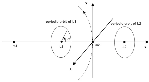
periodic orbit of L2 periodic orbit of L1

m2 α

yyyy

xxxx L1 L2

zzzz m1

2.3 Jacobi Integral

The restricted Hill three-body problem has an integral of motion similar to the CR3BP. Adding equations (2.9) - (2.11) after multiplying them by x, y,andz, respectively, we obtain

). (

3 3

2

2 xx yy zz

z r z x x z z y y x

x + + = ω −ω − ^µ + + ^(2.14)

Which, after integration, becomes,

^{2 2}

₍

₎

2 1 2

1 x z

v r

J = −^µ + ω − ^{, (2.15)}

where v= x²+ y²+z² is the velocity of the particle in the rotating frame, J is a constant called the Jacobi integral (Jacobi constant), which is a conservative quantity determined from the initial conditions. The value

of this constant has a strong influence on the dynamics of motion. The condition v² ≥0in Eq. (2.15) impose a restriction on the allowable position for the motion at any given value of J. Setting v=0 defines the zero- velocity surface, which sets a physical boundary of the allowable motion at a given value of J. In particular, the critical value of J at L1 and L2 defines the energy at which the zero-velocity surfaces open at L1 and L2, and is expressed as:

( )

2 ,

1 ⁹

2 1 µω

−

L =

J (2.16)

2.4 Normalization

Next, we normalize the above equations setting the unit length and the unit time as follows:

3 / 1

= 2

ω

l µ ^and

τ =ω^{1. (2.17)}

The normalized equations of motion (2.9)- (2.11) are then

3 3

2 r

x x y

x− = −

, (2.18)

2 3

r x y y+ =−

, (2.19)

r3

z z z+ =−

. (2.20)

This normalization allows us to eliminate all free parameters from the equations. Thus, computations performed for them can be scaled to any physical system by multiplying by the unit length and time, which only depend on the properties of the primary and secondary bodies. We may introduce again a pseudo- potential function

) ( ) 2(

3 ) 1

3 2( ) 1 , ,

( = ²− ² + +µ^{1/3 2}− ²+ ² +Ο µ^2/3

Ω x x y z

z r x z

y x

(2.21) and so the equations of motion (2.18)-(2.20) may be written as

x x

y

x =Ω

∂ Ω

=∂

− 2

, (2.22)

y y

x

y =Ω

∂ Ω

=∂ + 2

, (2.23)

z z

z =Ω

∂ Ω

= ∂

. (2.24)

Moreover, this normalization is equivalent to

ω

µ

( )

2 ,

1 ^{=± =±}

xL

(2.25)

... 16337 . 2 29

1 2/3 2

,

1 ^{=− =−}

JL

(2.26) Table 2.1 gives the normalized radius for the planets of the solar system. This is a quantity of interest as it defines the closest periapsis passage possible to the planet, and defines the periapsis radius where significant drag forces are available for an aerocapture spacecraft.

Table 2.1 Normalized Radius of the Solar System Planet

Planet Mass,

[kg × 10²³]

Gravitational parameter, [km³/s² × 10⁵]

Mean motion, [rad/s × 10^-7]

Normalized radius

Mercury 0.3302 0.220329 8.27 0.007663

Venus 4.869 3.248889 3.24 0.00415

Earth 5.9742 3.986345 1.99 0.002955

Mars 0.64191 0.428321 1.06 0.002173

Jupiter 1899 1267.127 0.168 0.000933

Saturn 568.8 379.5375 0.0676 0.000641

Uranus 86.86 57.9582 0.0267 0.000253

Neptune 102.4 68.32742 0.0121 0.000148

2.5 Linearized Equation of Motion around L1/L2 Points

ζ η

ξ = + = +

+

=x_L1,2 , y y_L1,2 , z z_L1,2 x

, (2.27)

where (x_L1,2,y_L1,2,z_L1,2) are the coordinates of the L1 and L2 points and (ξ,η,ζ) are the components of the position vector of the spacecraft relative to the L1/L2 points. The function Ω may be expanded around L1/L2 point, giving

). 3 ( ) , , ( )

, , ( )

, , (

) , ,

! ( 2 ) 1 , ,

! ( 2 ) 1 , ,

! ( 2 1

) , , ( )

, , ( )

, , ( ) , , (

2 , 1 2 , 1 2 , 1 2

, 1 2 , 1 2 , 1 2

, 1 2 , 1 2 , 1

2 2 , 1 2 , 1 2 , 1 2

2 , 1 2 , 1 2 , 1 2

2 , 1 2 , 1 2 , 1

2 , 1 2 , 1 2 , 1 2

, 1 2 , 1 2 , 1 2

, 1 2 , 1 2 , 1 2

, 1 2 , 1 2 , 1

Ο + Ω

+ Ω

+ Ω

+

Ω + Ω

+ Ω

+

Ω + Ω

+ Ω

+ Ω

= Ω

ζξ ηζ

ξη

ζ η

ξ

ζ η

ξ

L L L zx L

L L yz L

L L xy

L L L zz L

L L yy L

L L xx

L L L z L

L L y L

L L x L

L L

z y x z

y x z

y x

z y x z

y x z

y x

z y x z

y x z

y x z

y x

(2.28)

The differential equations of motion (2.13)-(2.15) become

ζ η ξ

ζ η

ξ η

ξ

0 0 0

2 , 1 2

, 1 2

,

1 ⁽²⁾

2

xz xy xx

L xz L

xy L

xx

Ω + Ω + Ω

≅

Ο + Ω

+ Ω

+ Ω

=

−

, (2.29)

ζ η

ξ ξ

η+2 =Ω_{yx L1,2} +Ω_{yy L1,2} +Ω_{yz L1,2} +Ο(2)

^{ξ η ζ}

ζ η

ξ ζ

0 0 0

2 , 1 2

, 1 2

,

1 ⁽²⁾

zz zy zx

L zz L

zy L

zx

Ω + Ω + Ω

≅

Ο + Ω

+ Ω

+ Ω

=

, (2.31)

where the symbols O(2) and O(3) stand for second-order term in ξ, η and ζ. Ω_{x L1,2}=Ω_{y L1,2}=Ω_{z L1,2} =0

since L1 and L2 are the equilibrium points. Moreover, since the L1 and L2 points are always on the x-axis, i.e.,

2 0

, 1 2 ,

1 ⁼ L ⁼

L ^z

y . Therefore, _Ω⁰_{xy =Ω}⁰_{yx =Ω}⁰_{xz =Ω}⁰_{zx =Ω}⁰_{yz =Ω}⁰_{zy =0}. Then, for the L1 and L2 points, equations (2.29)-(2.31) are simplified to

ξ η ξ−2 =Ω⁰_xx

, (2.32)

η ξ η+2 =Ω⁰_yy

, (2.33)

ζ ζ =Ω⁰_zz

. (2.34)

The in-plane characteristic equation associated with equations (2.32) and (2.33) is of the form

0 )

4

( ^{0 0 2 0 0}

4 _{+ −Ω −Ω +Ω Ω =}

yy xx yy

xx ^λ

λ

, (2.35)

and the in-plane eigenvalues can be expressed as

σ β β β

λ_1,2=± − ₁+ ₁²+ ₂² =±

, (2.36)

j xy

j β β β ω

λ_3,4=± ₁+ ₁²+ ₂² =±

, (2.37)

where β₁=2−(Ω⁰_xx+Ω⁰_yy)/2 ^and β₂ =−Ω⁰_xxΩ⁰_yy >0, and j is the imaginary unit. Additionally ω_xyis called the nondimensional frequency of the in-plane oscillatory mode.

The out-of-plane characteristic equation associate with equation (2.34) is

0 0

2_{−Ω =}

λ zz

, (2.38)

and the out-of-plane eigenvalues are

z

zz ^j

j ω

λ_5,6 =± |Ω⁰ |=±

, (2.39)

where ω_zis called the nondimensional frequency of the out-of-plane oscillatory mode. At L1 and L2 points in the Hill model, we have

4 ,

3 ,

9 ^{0 0}

0 _{= Ω =− Ω =−}

Ω_{xx yy zz}

, (2.40)

and the eigenvalues are

508 .

2 2

,

1 ^{=±σ ≅±}

λ

, (2.41)

072 .

4 2

,

3 ^=±jωxy ^=±j

λ

, (2.42)

6 2

,

5 ^=±jωz ^=±j

λ

. (2.43)

The general solutions for ξ and η are

=

=

4

1 i

t i

e i

A ^λ ξ

, (2.44)

=

=

4

1 i

t i

e i

B ^λ η

, (2.45)

where A_i and B_i are constant, but not independent. Direct substitution of equations (2.44)-(2.45) into equations (2.32)-(2.33) results in the following relation between Ai and Bi, that is,

.

i i i i

xx i

i ^{A A}

B α

λ

λ ^−Ω =

= 2

0 2

, (2.46)

and at the initial time,

=

=

4

1 0

0

i t i

e i

A ^λ ξ

, (2.47)

=

=

4

1 0

0

i

t i i

e i

A ^λ λ ξ

, (2.48)

=

=

4

1 0

0

i

t i i

e i

A ^λ α η

, (2.49)

=

=

4

1 0

0

i

t i i i

e i

A ^λ λ α η

. (2.50)

Selecting initial conditions such that A1 = A2 = 0, particular solutions containing only sine and cosine functions of the time for ξ and η are obtained,

t

t _xy

xy ^ω

β ω η ξ

ξ cos sin

3 0

0 ⁺

=

, (2.51)

t

t _xy

xy ^ω

β ω ξ η

η cos sin

3 0

0 ⁺

=

, (2.52)

where

xy xx xy

ω β ω

2

0 2 3

Ω

= − ^.

On the other hand, the general solution for can be written in the following form,

t

t _z

z

z ^ω

ω ω ζ ζ

ζ = ₀cos − ⁰ sin

(2.51) From the linear approximation, the three-dimensional motion of spacecraft is not periodic since the in-plane and out-of-plane frequencies are not commensurate. However, _ωxy and ω_z are relatively close in value for the problem of interest. This suggests that quasi-periodic motion can be approximated.

2.6 Periodic Orbits in the vicinity of the Libration Points

There exist periodic orbits near the libration points in the two- and three-dimensional space [33-37] called Lyapunov and Halo orbits, respectively, whose sizes depend on the value of the Jacobi constant (see Fig. 2.2). If a spaceport is built on a Halo orbit about the L2 point, it is not hidden in the shadow of the secondary body

because the radius of the Halo orbits can be made larger than that of the secondary body. Thus, we will only consider the Halo orbit transfer case.

The computation of periodic orbits is generally time consuming unless a good initial guess is already available. Thus, development of a numerical method to improve an initial guess by predicting behavior near the reference solution is desirable. Such a method requires the information concerning the sensitivity of the state from changes in the initial guess. To gain insight into the sensitivities, it is useful to examine the evolution of a state vector by the state transition matrix in the vicinity of a reference solution. If a periodic orbit exists, it is possible to linearize about the periodic orbit. Equations (2.22)-(2.24) can be rewritten as six first-order differential equations where a state vector is defined as q=[x y z x y z]^T.

) (q f q=

. (2.52)

Given some reference solution, _qref, to the differential equations, an approximation for the variations relative to the reference solution can be derived through a first-order Taylor series expansion about the reference. Ignoring the high order terms, the resulting linearized state variational equations are written as

) ( ) ( )

(t At q t

q δ

δ =

, (2.53)

where

qref

q t f

A ∂

=∂ )

( ^{is a 6} × 6, generally time-varying, matrix. It can be written in term of the following four 3

× 3 sub matrices,

= Ω

C t I

A

ij

0 3

) (

, (2.54)

where 0 represents the zero matrix and I3 is the identity matrix. The C is defined as constant,

−

=

0 0 0

0 0 2

0 2 0 C

, (2.55)

and Ωij has the form,

Ω Ω Ω

Ω Ω Ω

Ω Ω Ω

= Ω

zz zy zx

yz yy yx

xz xy xx

ij

, (2.56)

where the subscripts indicate second partial derivatives of the pseudo-potential evaluated on the reference solution. The solution to the linearized Equation (2.53) is

) ( ) , ( )

(t t t₀ qt₀

q δ

δ =Φ

, (2.57)

where Φ(t,t₀) is the state transition matrix (STM). The expression in Eq. (2.57) relates variations in the trajectory at time t to the initial perturbation at time t0. The STM is also described as a sensitivity matrix since it offers a linear prediction of the sensitivity of the trajectory to initial variations. Next, we consider the Poincaré section, Σ, which is transverse to the flow in three-dimensional space and reduces the dimension of the phase space by one (see Fig. 2.3). From some set of initial conditions in the Poincaré section, we propagate the equation of motions. At the time that the path crosses this section again, an intersecting point marks on this section. This point reflects a second crossing of the section. Thus, the point in the section is denoted a return map (Poincaré map). Therefore, the periodic orbit would be represented in this section by a single point, denoted as a fixed point, q^*(the periodic orbit intersects the same location in the section on every pass). Supposing the crossing period T, from Eq. (2.57),

) ( ) , ( )

(t₀ T t₀ T t₀ q t₀

q δ

δ + =Φ +

, (2.58)

where Φ(t₀+T,t₀)is called the Monodromy matrix. This Monodromy matrix is a linear stroboscopic map for the fixed point in the vicinity of the reference trajectory.

In this study, we compute the Halo orbits as follows. First, we assume the initial condition is

(

)

)

(t₀ x₀ z₀ y₀

q = . Using the Runge-Kutta-Fehlberg method, the equations of motion are integrated keeping an allowance error below fourteenth-order until the sign of y changes twice, and the time at this point

is defined to be t. If q(t₀ +t)=

(

)

Figure 2.2: A few Halo orbits around L1.

Figure 2.3: Periodic orbit and Poincaré section.

2.7 Invariant Manifold

There exist invariant structures associated with these periodic orbits, called unstable and stable manifolds [38, 39, 43]. These are trajectories that depart from or wind onto the periodic orbit with a nearly zero velocity correction, depending on whether they are stable or unstable, respectively. We exploit the unstable manifolds for escape trajectories from Halo orbit and the stable manifolds for capture trajectories to Halo orbits (see Fig. 2.4).

To obtain the manifolds, stability information associated with the periodic orbit, contained within the Monodromy matrix, is examined. According to Floquet theory [44], the STM can be rewritten as,

) ( ) ( ) ,

(t t₀ =F t e^BtF⁻¹ t₀ Φ

, (2.59)

where F(t0) is a periodic matrix and B is a constant diagonal matrix. After one period, where t = t0 + T, F(t0+T) = F(t0), Eq. (2.59) can be rewritten as,

) ( ) , ( )

(_{0 0 0 0}

1 ) (₀

t F t T t t F

e^Bt+T = ⁻ Φ +

. (2.60)

Therefore, F(t0) and B contain the eigenvectors, ν_i , and the eigenvalues, λi, of the Monodromy matrix. The eigenvalues of the Monodromy matrix offer information about the phase space in the vicinity of the periodic

orbit because λi reflect the linear stability of the fixed point in the map. According to Lyapunov's Theorem, since the determinant of the Monodromy matrix is equal to one, the eigenvalues of the Monodromy matrix must occur in reciprocal pairs. Furthermore, one pair of eigenvalues must be equal to one at least because the orbit is periodic and any complex eigenvalue must be paired with its conjugate. For periodic orbits in the CR3BP, λ1 = λ2 = 1, λ3 and λ4 are complex conjugate eigenvalues located on the unit circle, and λ5 and λ6 are real with λ5 = λ6

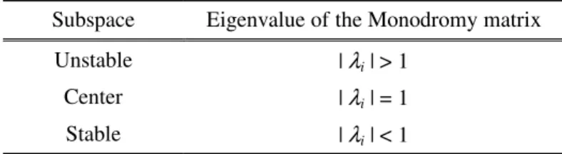
-1. The flow in the region of phase space near a periodic orbit can be decomposed into three subspaces: the stable, unstable and center subspaces (E^s, E^u, E^c). Table 2.2 shows a relation between the subspace and the eigenvalues of the Monodromy matrix. Eigenvectors corresponding to a stable eigenvalue lie in the stable subspace and yield stable manifolds asymptotically approaching the periodic orbit as t→∞. Eigenvectors corresponding to an unstable eigenvalue lie in the unstable subspace and yield unstable manifolds asymptotically approaching the orbit as t→−∞. Eigenvectors corresponding to a center eigenvalue lie in the center subspace and yield trajectories neither approaching nor departing the periodic orbit as t→±∞. The directions defined by the eigenvectors associated with the stable/unstable subspace of the linear system are used to approximate the direction of the local stable and unstable manifolds. The local stable/unstable manifolds, Wl^s and Wl^u, are then propagated forward/backward in time to compute approximations to the global stable/unstable manifolds in the nonlinear system (W^s and W^u). At a fixed point, q , corresponding stable and ^* unstable eigenvectors, ν^s(q^*)and ν^u(q^*)are computed from the Monodromy matrix and normalized with respect to its position, these are,

2 2 2

z s s

s s

n x +y +z

= ^ν

ν

, (2.61)

2 2 2

u u u

u u

n x +y +z

= ^ν

ν

. (2.62)

The initial state vectors for the local stable and unstable manifolds are expressed as,

s n

s q d

q₀ = ^*± ν

, (2.63)

u n

u q d

q₀ = ^*± ν

, (2.64)

where d is the initial displacement from the periodic orbit. The initial displacement must be small enough to justify the linear approximation. A shift in the +ν_n^sdirection results in manifolds Wl

s+ and Wl

u+, while the shift

in the -ν_n^sdirection results in manifolds W_l^s- and W_l^u-. Thus, q₀^sand q₀^uare used to propagate forward/backward in time, and these propagation creates the global stable/unstable manifolds, W^s+, W^s-, W^u+ and W^u- (see Fig. 2.5). Moreover, the global manifold is computed for each fixed point along the periodic orbit, the manifold surface is generated. In this paper, invariant global manifolds are generated by applying an infinitesimal impulse (the value of 0.00001 km/s in the Sun-Mars system) at each fixed point along the Halo orbit and integrated forward/backwards in time. The location on the periodic orbit is parameterized by a phase angle α on the periodic orbit (see Fig. 2.1).

Table 2.1: Relation between the subspace and the eigenvalue of the Monodromy matrix Subspace Eigenvalue of the Monodromy matrix

Unstable | λi | > 1

Center | λi | = 1

Stable | λi | < 1

Figure 2.4: Stable manifold around L1 (represented until first Periapsis Point).

Figure 2.5: Stable and unstable manifolds tangent to eigenvectors.

CHAPTER 3

3 Escape and Capture Trajectories from and to Halo Orbits

3.1 Assumption of Escape Trajectories

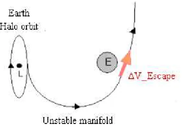
In this study, we define that escape trajectories are trajectories that leave from a Halo orbit around Sun-Earth L1 or L2 using unstable manifolds and approach the Earth. Subsequently, at closest approach an impulsive maneuver is performed to escape from the Earth’s gravitational dominance and put the spacecraft on an interplanetary trajectory (Fig. 3.1). The reason why an impulsive maneuver is performed near the surface of the Earth (perigee) is because it is the energetically efficient place to increase the escape energy. In this way, the unstable manifolds are used for escape trajectories from Halo orbits.

Figure 3.1: Example of escape impulsive trajectory from the Earth Halo orbit.

3.2 Assumption of Capture Trajectories

On the other hand, we assume that capture trajectories are trajectories that enter the sphere of influence of a target body from the interplanetary space and have a close flyby with the target body. At closest approach an impulsive maneuver is performed to put the spacecraft on a stable manifold that leads to capture to a Halo orbit around L1 or L2 of the target body (Fig. 3.2). The reason why an impulsive maneuver is performed near the surface of the target body (periapsis) is because this is the energetically efficient place to reduce the approach

energy, which may also be reduced by using an aero assist with the planetary atmosphere. Once placed on the stable manifold, the S/C approaches the Halo orbit, perhaps orbiting around the target body several times on its way. Once it is close to and crosses the Halo orbit a negligible impulsive maneuver is necessary to place it on the Halo orbit completely. In this way, the stable manifolds are used for capture trajectories to Halo orbits.

Figure 3.2: Example of capture impulsive trajectory to the Mars Halo orbit.

3.3 Characteristics of Periapsis Points of Invariant Manifolds

In this section, we investigate the first four periapsis passage points of invariant manifolds where an impulse maneuver may be performed for an interplanetary transfer. Unstable manifolds propagate forwards from a certain point on the Halo orbits in time. On the other hand, stable manifolds propagate backwards from a certain point on the Halo orbits in time.

3.3.1 Periapsis Location

Figure 3.3 shows an example of the first four periapsis passage points of one example trajectory of the L1 stable manifold (J = -2.01). The secondary body is located at the origin. Based on this result, Fig. 3.4 plots the first four periapsis point’s locations of the L1 Halo stable manifold for several values of the Jacobi constant (i.e., the size of Halo orbits). The periapsis locations of stable and unstable manifolds of a L1/L2 Halo orbit are

symmetric to the x-z plane. Moreover, the periapsis locations of L1 unstable and L2 stable manifolds are symmetric to the y-z plane, and vice versa. We can see that each periapsis point region spreads out and that these periapsis locations depend on the value of the Jacobi constant.

Figure 3.3: First four periapsis points of an example trajectory of the L1 stable manifold propagated backward from a certain point on the Halo orbit.

a) J = -2.01

b) J = -1.84

c) J = -1.75

Figure 3.4: First four periapsis locations of L1 Halo stable manifold. The secondary body is located at the origin.

3.3.2 Minimum Periapsis Distance

Figure 3.5 shows a relation between a minimum periapsis distance and the value of the Jacobi constant. The minimum periapsis distance means the distance from the origin to the periapsis point of stable manifold, which is closest to the origin in each of the four periapsis points in the same value of the Jacobi constant. The minimum periapsis distance decreases as the value of the Jacobi constant increases, and each four minimum periapsis distance becomes smaller than 0.000148 (which is smaller than the smallest normalized planetary radius, Neptune) when the value of the Jacobi constant is large. Thus the stable and unstable manifold of the first four periapsis passage points can intersect the surface of any of the planets in the solar system (but the size of the Halo orbit is limited). That is to say, a spacecraft can depart from the Halo orbit and approach the surface of the planet with the negligible velocity correction, and wind into the Halo orbit from the surface of the planet with negligible velocity correction by changing the size of the Halo orbit.

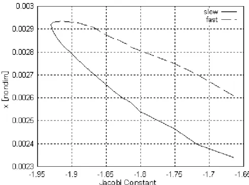
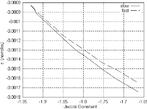
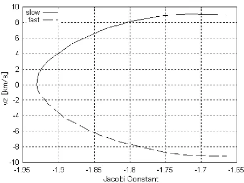
3.3.3 Fast and Slow Transfer

In the same size of Halo orbits, there exist fast transfers and slow transfers which have same altitude of periapsis (Pf and Ps) as shown in Figs 3.6 and 3.7. These TOF from a Halo orbit to periapsis are different (e.g., fast transfer to Pf = 1.74 years, slow transfer to Ps = 1.86 years). They are obtained by different initial positions at a Halo orbit.

Figure 3.6: Fast and slow transfers between planet’s periapsis and Halo orbit.

Figure 3.7: Periapsis of fast and slow manifold transfers.

3.3.4 Position and Velocity of Periapsis near the Surface of Planets

Next, Figs 3.8 – 3.13 show the position and the speed of the first periapsis of the Earth “L1” unstable manifolds near the Earth surface (altitude = 300 km) as a function of the Jacobi constant in the Sun-Earth fixed frame. The x and y components of position and velocity of Earth “L2” unstable manifolds is symmetric to that of Earth “L1” unstable manifolds. According to the Fig. 3.13, since the z direction component of velocity increases as the value of the Jacobi constant (the size of Halo orbits) increases, we should select small size Halo orbits. At this time, the y direction component of velocity is positive with the small value of the Jacobi constant form Fig. 3.12.

On the other hand, Figs 3.14 – 3.19 show the position and the velocity of the first periapsis of the Mars “L2” stable manifolds near the Mars surface (altitude = 200 km) as a function of the Jacobi constant in the Sun-Mars fixed frame. In the same way as the Earth unstable manifolds, we should select small Halo orbits since the z direction component of velocity increases as the value of the Jacobi constant increases as shown in Fig. 3.19.

Figure 3.8: x-coordinate of periapsis of Earth L1 unstable manifolds as a function of the Jacobi constant.

Figure 3.9: y-coordinate of periapsis of Earth L1 unstable manifolds as a function of the Jacobi constant.

Figure 3.10: z-coordinate of periapsis of Earth L1 unstable manifolds as a function of Jacobi constant.

Figure 3.11: vx component of periapsis velocity of Earth L1 unstable manifolds as a function of the Jacobi constant.

Figure 3.12: vy component of periapsis velocity of Earth L1 unstable manifolds as a function of the Jacobi constant.

Figure 3.13: vz component of periapsis velocity of Earth L1 unstable manifolds as a function of the Jacobi constant.

Figure 3.14: x-coordinate of periapsis of Mars L2 stable manifold as a function of the Jacobi constant.

Figure 3.15: y-coordinate of periapsis of Mars L2 stable manifold as a function of the Jacobi constant.

Figure 3.16: z-coordinate of periapsis of Mars L2 stable manifold as a function of the Jacobi constant.

Figure 3.17: vx component of periapsis velocity of Mars L2 stable manifold as a function of the Jacobi constant.

Figure 3.18: vy component of periapsis velocity of Mars L2 stable manifold as a function of the Jacobi constant.

Figure 3.19: vz component of periapsis velocity of Mars L2 stable manifold as a function of the Jacobi constant.

3.4 Comparison with Periapsis of Trajectories from/to L1 or L2 Points

By way of comparison, we consider a two-impulse transfer from the Sun-Earth L1/L2 point to the Earth (altitude = 300 km). In Fig. 3.20, there exist two classes of ballistic transfers; one is a fast transfer (∆V is around 342 m/s at L1/L2 and the TOF is around 35 days), the other is a slow transfer (∆V is around 279 m/s at L1/L2 and the TOF is around 117 days) [12]. On the other hand, the required ∆V at Halo orbit for the transfer from the Halo orbit to Earth is almost zero. Moreover, the magnitude of velocity at perigee from L1/L2 points is almost the same as that of the transfer from Earth Halo orbit. Therefore, it is better to put the spaceport on the Halo orbit of Earth and a target body than to put on L1/L2 point from the view of the ∆V.

Figure 3.20: Transfer between L1 point and secondary body.

3.5 Summary

First, we defined the escape and capture trajectories from/to Halo orbit using the impulsive maneuver at the periapsis of manifold. And then, the characteristics of the periapsis of manifold, where an impulsive maneuver would be performed for the interplanetary transfer, were investigated. As a result, the stable and unstable manifolds could intersect the surface of any of the planets by changing the size of the Halo orbits. Namely, a spacecraft could leave the Halo orbit and come close to the surface of the planet with the negligible velocity correction, and wind into the Halo orbit from the surface of the planet with negligible velocity corrections. Moreover, the position and the velocity of the manifold at periapsis near the surface of planets are discussed.

CHAPTER 4

4 Reduction of the Time of Flight for Escape and Capture from/to Halo Orbit

In the previous chapter, the periapsis of stable and unstable manifolds associated with the Halo orbits are investigated. As a result, it was found that the impulsive maneuver could be performed at the surface of any of the planets in the solar system using the unstable and stable manifolds. However, the time of flight (TOF) is long for our escape and capture on the Halo orbit using the unstable and stable manifold because the manifolds generally orbit around the L1/L2 point several times. For instance, the TOF is approximately 1.9 years for the capture using stable manifold from Mars periapsis to the arrival point on the Halo orbit in Fig. 4.1, where the points in the figure are plotted every month. It is not feasible, thus a reduction of the TOF for the escape and the capture is discussed.

Figure 4.1: Example capture trajectory to Mars Halo orbit for J = -2.01

4.1 Time of Flight Reduction

We assume performing Vperi and VHO at both the periapsis of manifold and the point on Halo orbit, respectively, to reduce TOF for escape and capture (two-impulse escape and capture as shown in Fig. 4.2). Here, we focus on the capture case, but a similar method can be followed for the escape case. As the total V ( Vperi + VHO) increases, the shape of the capture trajectories varies as shown in Fig. 4.3 (the values are for the capture to Mars Halo orbit). As mentioned in chapter 3, there exist two families of the capture trajectories approaching Mars. We define the trajectory family as the slow captures (S), and the trajectory family as the fast captures (F). Figure 4.4 plots the TOF against the required total V for the capture from Mars periapsis to the Halo orbits. Each parabola line means the relation between the TOF and the required total V with respect to each arrival point where is performed VHO. The vertex of a parabola represents the minimum required V with respect to the arrival point (Figure 4.5). In fact, depending on the applied direction, TOF not only increases but also decreases as the total V to reach each arrival point in Fig. 4.6 increases. From this result, TOF could be reduced more than a year by performing a V of only 0.06 km/s. It is a significant improvement by performing a decent V. Moreover, it was found that TOF has a linear relation with the logarithm of the minimum required V in the both slow and fast capture families. Even changing the size of Halo orbits, TOF also has a linear relation with the logarithm of the minimum required V (see Fig. 4.7).

(S-1) ∆∆V = 2.22e-5 km/s & TOF = 1.28 years ∆∆

(F-1) ∆∆V = 4.08e-5 km/s & TOF = 1.21 years ∆∆

(S-2) ∆∆V = 1.28e-4 km/s & TOF = 1.05 years ∆∆

(S-3) ∆∆V = 6.37e-4 km/s & TOF = 0.82 years ∆∆

(F-3) ∆∆V = 1.18e-3 km/s & TOF = 0.75 years ∆∆

(S-4) ∆∆V = 3.43e-3 km/s & TOF = 0.59 years ∆∆

(F-4) ∆∆V = 5.87e-2 km/s & TOF = 0.53 years ∆∆

(S-5) ∆∆V = 2.44e-2 km/s & TOF = 0.36 years ∆∆

(F-5) ∆∆V = 3.79e-2 km/s & TOF = 0.32 years ∆∆

Figure 4.3: Shape of the capture trajectories as increasing V in the x-y plane.

Figure 4.4: Relation between the TOF and V (J = -1.85)

Figure 4.5: Minimum required V for the capture to the arrival point

Figure 4.6: Capture trajectories of minimum required V and others.

Figure 4.7: Relation between the TOF and V (Changing the size of Halo orbits).