本文総合研究大学院大学学術情報リポジトリ甲1410 本文

(1)

Vortices, Zonal Flows, and Transport

in Gyrokinetic Plasma Turbulence

Motoki Nakata

DOCTOR OF PHILOSOPHY

Department of Fusion Science

School of Physical Science

The Graduate University for Advanced Studies

March, 2011

(2)

(3)

To Osaya

(4)

(5)

Acknowledgements

F

irst of all, I would like to express sincere gratitude to my advisers Professor Tomo-Hiko Watanabe and Professor Hideo Sugama for their guidance, support, and encouragement over five years of my doctoral course. Especially, I really do appreciate their unlimited generosity to my interest in different fields of physics, and to my inefficiency and unskillful- ness. It is my great pleasure to compile the doctoral dissertation as an accumulation of many discussions with them.

I would also like to extend my appreciation to Professor Wendell Horton of Institute for Fusion Studies, The University of Texas at Austin for his kind and fruitful suggestions. I am deeply honored to share the strong interest in complicated, but beautiful nature of vortices in plasma turbulence with the great plasma physicist.

Special thanks goes to Professor Yasuaki Kishimoto (Kyoto univ.), Dr. Jiquan Li (Kyoto univ.), Dr. Kenji Imadera (Kyoto univ.), Dr. Yasuhiro Idomura (JAEA), Dr. Nobuyuki Aiba (JAEA), Dr. Ken Uzawa (JAEA), Dr. Akihiro Ishizawa (NIFS), Dr. Shinsuke Satake (NIFS), Dr. Ryutaro Kanno (NIFS), Dr. Masanori Nunami (NIFS), Dr. Atsushi Ito (NIFS), Dr. Seiya Nishimura (NIFS), and Dr. Gakushi Kawamura (NIFS), who have provided me with useful comments on this study and also discussed various topics in physics, mathematics, politics, and history.

Furthermore, I thank Dr.(to be) Seikichi Matsuoka, Dr.(to be) Kunihiro Ogawa, and the other Ph.D students in NIFS for mutual encouragement, and for sharing hopes and concerns about the future. And I am sincerely grateful to my family and friends for their support and understanding.

Finally, I absolutely love day-to-day lives in Toki-city!

This work is supported by Grant-in-Aid for Japan Society for the Promotion of Science Fel- lowship (No. 20-4017). Numerical computations are performed on the NIFS Plasma Simulator and Supercomputing Resources at Cyberscience Center of Tohoku University.

(6)

(7)

Abstract

P

lasma turbulence driven by drift wave instabilities is a key issue for understanding anomalous transport of particle, momentum, and heat observed in magnetically confined plasmas. Ion temperature gradient (ITG) and electron temperature gradient (ETG) driven instabilities are considered as main causes of the micro-scale turbulence with the spatial scale of the ion and electron gyroradii, respectively. Various flow structures, i.e., fine-scale turbulent vortices, axisymmetric zonal flows, and radially elongated streamers, are generated through complicated nonlinear interactions in plasma turbulence. From the aspect of regulating the turbulent transport in future burning plasmas, it is worthwhile to understand fundamental physics behind the formation of vortex and zonal flow structures and their stability as well as the related transport properties. Since the high temperature plasmas with weak collisionality inherently involve a lot of kinetic processes, i.e., the Landau damping, the finite gyroradius effect, the particle drift, and the magnetic trapping, the gyrokinetic theory is a powerful method for the precise investigation of the physical mechanisms of plasma turbulent transport.

In this dissertation, the ITG and ETG turbulence are explored based on nonlinear gyrokinetic theory and direct numerical simulations. Then, the results concerning (i) formation of coherent vortex streets and the resultant transport reduction, (ii) effects of parallel dynamics on the zonal flow generation, and (iii) nonlinear entropy transfer among turbulent vortices and zonal flows, are presented.

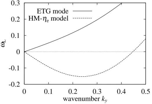
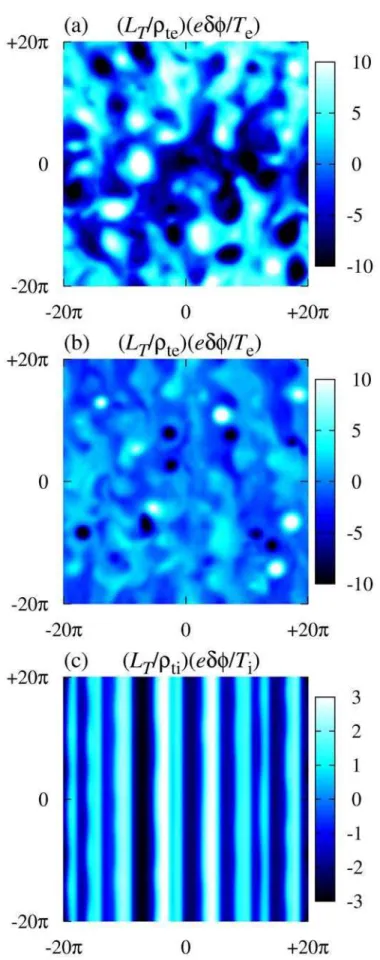
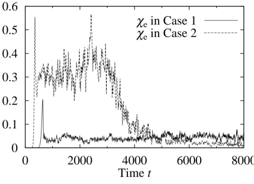
First, vortex structures in the slab ETG turbulence are investigated, including comparisons with those in the slab ITG case. Depending on parameters which determine the growth rate of linear ETG modes, two different flow structures are observed, i.e., statistically steady turbulence with a weak zonal flow and coherent vortex streets along a strong zonal flow. The former involves many isolated vortices with complicated motion and their mergers, which leads to steady electron heat transport. When the latter is formed, the high wavenumber components of potential and temperature fluctuations are reduced, and the electron heat transport decreases significantly. It is found that the transport reduction is mainly associated with the phase matching between the potential and temperature fluctuations rather than the reduction of fluctuation amplitudes. A traveling wave solution of a Hasegawa-Mima type equation derived from the gyrokinetic equation with the electron temperature gradient agrees well with the coherent vortex streets found in the slab ETG turbulence.

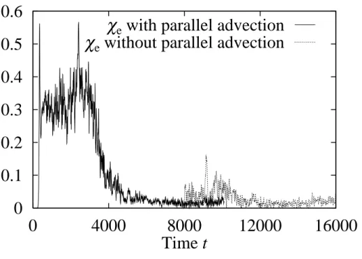
Second, effects of parallel dynamics on transition of vortex structures and zonal flows, which are closely associated with transport reduction found in the slab ETG turbulence, are intensively

(8)

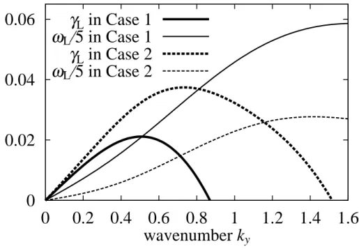
zonal-flow-dominated state, depending on the relative magnitude of the parallel compression to the diamagnetic drift. In particular, the formation of coherent vortex streets is correlated with strong generation of zonal flows for the cases with weak parallel compression, even though the maximum growth rate of linear ETG modes is relatively large. A physical mechanism of the secondary growth of zonal flows is discussed based on the modulational instability analysis with a truncated fluid model, where the parallel dynamics with acoustic modes is incorporated. The modulational instability for zonal flows is found to be stabilized by the effect of the finite parallel compression. The theoretical analysis qualitatively agrees with the secondary growth of zonal flows found in the slab ETG turbulence simulations, where the transition of vortex structures is observed.

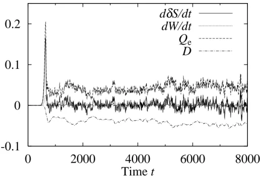
Finally, the investigations of vortex structures and zonal flows are extended to toroidal ITG and ETG turbulence by means of five-dimensional nonlinear gyrokinetic simulations. In the steady state, the formation of the strong zonal flow is observed in the toroidal ITG turbulence, while the radially elongated streamers, which yield the significant enhancement of heat transport, develop in the toroidal ETG case. Gyrokinetic entropy balance relations for zonal and non-zonal modes, and the nonlinear entropy transfer function, which is regarded as a kinetic extension of the zonal-flow energy production due to the hydrodynamic Reynolds stress, are carefully examined. The different entropy transfer processes in saturation and steady phases are revealed for the ITG turbulence. The entropy transfer from non-zonal to zonal modes is substantial in the saturation phase of the instability growth, while the entropy transfer to zonal modes becomes quite weak in the steady phase. Instead, the entropy variable of the low radial-wavenumber modes driving the heat transport are successively transferred to the higher radial-wavenumber modes with less contribution to turbulent heat flux via the strong interaction with zonal flows. On the other hand, in both the saturation and steady phases of the ETG turbulence, the catalytic role of zonal flows in the entropy transfer to the higher radial-wavenumber modes is much weaker than that in the ITG case. Then, the entropy transfer processes among low-wavenumber non-zonal modes including radially elongated streamers are dominant and the higher heat transport level is sustained.

The formation of vortices and zonal flows, and the related entropy transfer processes in the ITG and ETG turbulence are comprehensively examined in this study, then the transport regula- tion due to the nonlinear interactions with zonal flows are clarified in the framework of kinetic theory. The results obtained by a novel method of the entropy transfer analysis provide one with not only deeper understandings of the physics of the turbulent transport and zonal flows, but fruitful suggestions for advanced turbulence diagnostics such as the bi-spectrum analysis.

(9)

(10)

The one who doesn't go backward goes forward.

(11)

Chapter 1 Introduction

D

rift wave turbulence driven by micro-instabilities is a key issue for understanding and predicting anomalous (or turbulent) transport of particle, momentum, and heat in the core region of magnetically confined plasmas, where the experimentally observed transport level is much higher than that predicted from both the classical and neoclassical transport theory based on Coulomb collision processes of ions and electrons [1]. In particular, the turbulent heat transport determines the energy confinement time which is directly connected to the quality of future fusion reactors so that tremendous efforts have been devoted so far to theoretical prediction, numerical simulations and dedicated experiments. Since the dynamics of turbulent vortices and the related transport processes in high temperature plasmas with weak collisionality are inherently nonlinear, and involve a lot of kinetic processes, i.e., the Landau damping, the finite gyroradius effect, the particle drift, and the magnetic trapping, the direct numerical simulations by means of an appropriate kinetic model are indispensable for understandings of physical mechanisms of plasma turbulent transport and for quantitative estimation of the transport level. The gyrokinetic model (for example, see Ref. 2 – 4) is a reduced kinetic equation averaged over the fast gyromotion without losing important kinetic effects described above, and is the most reliable and useful kinetic description of the nonlinear dynamics of low-frequency turbulence in collisionless (or weakly collisional) magnetized plasmas.

In general, magnetically confined plasmas with high ion and electron temperature involve various fluctuations observed in a wide range of spatial scales, and the turbulent transport is considered to be driven by micro-instabilities originated from inhomogeneities of density, temperature, and magnetic fields, where the scale lengths related to ion and electron gyroradii are much shorter than the equilibrium scales. Drift waves are destabilized by the equilibrium density and temperature gradients above thresholds, even if the plasma equilibrium is stable to the macroscopic instabilities such as MHD modes. Then, the turbulent vortices with various spatial

1

(14)

scales develop through the complicated nonlinear interactions due to E× B convective flows. The ion temperature gradient (ITG) driven mode, which is one of the micro-instabilities, is considered to be a main cause of the turbulent ion heat transport in the core region of tokamak and helical plasmas, and the ITG turbulence has been extensively investigated by means of numerical simulations based on gyrokinetic and gyrofluid models [5–13]. The spatial scales of the ITG turbulence perpendicular to the confinement magnetic field are of the order of ion gyroradii, and the phase velocity is basically associated with the ion diamagnetic drift motion. One of the remarkable results obtained by the ITG turbulence simulations is that the meso-scale zonal flows, which are spontaneously generated through the nonlinear interactions among turbulent fluctuations, effectively suppress the turbulent heat transport by the strong flow shear in the radial direction. Intensive simulation studies have confirmed that the transport reduction by zonal flows leads to the nonlinear up-shift of the critical temperature gradient which is larger than the linear stability threshold of the ITG modes (that is, so-called Dimits shift) [14]. The self-generated zonal flow in the plasma turbulence is now recognized as a key constituent of a “drift-wave – zonal-flow system”. Existence of ion-scale zonal flows has been revealed by a direct measurement of spatial structures of electrostatic potential fluctuations in laboratory experiments [15].

Zonal flows are nonlinearly generated through the Reynolds stress in the drift-wave turbulence. The detailed physical mechanisms of the zonal flow generation have discussed from the view point of the nonlinear parametric instabilities through coupling of zonal flows and coherent drift waves [16, 17], or the Kelvin-Helmholtz (K-H) instability of radially elongated drift-wave vortices [18, 19]. The zonal flow generation is, thus, regarded as a “secondary” instability by contrast with the primary drift-wave instability. For the saturation of the zonal-flow growth in drift-wave turbulence, several mechanisms have been discussed (reviewed in Ref. 20). General- ized K-H instability, which is regarded as a “tertiary” instability, is one of the candidates for a saturation mechanism of zonal flows in the ITG turbulence [18,19]. Furthermore, the importance of parallel flows and viscosity in the zonal flow dynamics has also been pointed out [21, 22].

The electron temperature gradient (ETG) driven mode is the counterpart of the ITG mode, and the ETG turbulence is considered as a possible cause of the electron heat transport. How- ever, the gyro-Bohm scaling for the ETG turbulence with T_e= T_i predicts the smaller electron heat transport by a factor of ^√m_e/m_i than the ion heat transport driven by the ITG turbulence, where T_sand m_smean the temperature and the mass of ions (s = i) and electrons (s = e), respectively. Many experimental observations, nevertheless, commonly indicate the strong anomaly of the electron heat transport, which is of the same order as the ion one. Even when the ion heat transport is reduced by the internal transport barrier [23, 24], the anomalous electron heat

(15)

3 transport is still observed. From the view point of theoretical model, the linear ETG modes with an adiabatic ion response are isomorphic to the linear ITG modes with an adiabatic electron response. However, the nonlinear evolution of the ETG instability is crucially different from that of the ITG one, because the intensity of nonlinearly generated zonal flows in the ETG turbulence is much lower than that in the ITG turbulence. In the ITG turbulence, since the electron gyroradius is negligibly smaller than the radial wavelengths of the zonal-flow potentials, the radial motion of the electrons can not shield the zonal-flow potentials which are constant on a flux surface. Thus, the ITG-driven zonal flows with high amplitude can develop. On the other hand, in the ETG turbulence, the radial motion of ions resulted from the large gyroradius shields the zonal- flow potentials. The different radial motion of the background species (electrons for the ITG case, or ions for the ETG case) is, thus, responsible for the different zonal-flow generations, and higher transport level in the gyro-Bohm unit is observed in the ETG turbulence [25]. Further- more, the ETG turbulence involves various vortex structures, such as turbulent vortices, zonal flows, and radially elongated streamers, of which the appearance strongly depends on geomet- rical and plasma parameters [26]. Recently, a number of gyrokinetic simulations of the toroidal ETG turbulence have been performed and benchmarked with various simulation codes [25–31]. Especially, the nonlinear dynamics of streamers, which may lead to substantial enhancement of the heat transport in toroidal systems, has been actively pursued [25, 29]. Nevertheless, the saturation mechanism of the toroidal ETG instability under the strong magnetic shear and the estimation of resultant transport level are still open problems.

From the aspect of the turbulence-control with regulating the turbulent heat transport in the future fusion plasmas, it is worthwhile to understand fundamental physics behind the formation of vortex structures including zonal flows and their stability as well as the related transport properties. One of the objectives of this study is elucidating what kind of the vortex structures enhance or suppress the turbulent transport, and how the zonal flows play a role in the transport suppression in the ITG and ETG turbulence in the framework of gyrokinetic theory. We believe that detailed analyses of the vortex structures and the velocity-space structures of the distribution function are necessary for better understandings of the underlying turbulent transport processes in high temperature plasmas. To this end, vortex and zonal flow structures and velocity-space structures of the distribution function in the slab/toroidal ITG/ETG turbulence are extensively explored based on nonlinear gyrokinetic theory and the direct numerical simulations. The five-dimensional nonlinear gyrokinetic Vlasov simulations with high phase-space resolution enable us to examine in detail the gyrokinetic entropy balance relation and the associated entropy transfer processes which provide ones with deeper physical insight into the nonlinear interaction between drift-wave turbulence and zonal flows as well as the associated transport processes.

(16)

The outline of this dissertation is given as follows. First, gyrokinetic models and the entropy balance relation used in the present study are briefly described in Chap. 2. In Chap. 3, vortex structures in the slab ETG turbulence are investigated, including comparisons with those in the slab ITG case. Then, formation of the coherent vortex streets, which is closely associated with the transport reduction, in the slab ETG turbulence is discussed in detail. In Chap. 4, effects of parallel dynamics on the transition of vortex structures and zonal flows are intensively examined by the comprehensive parameter studies. Also, the physical mechanism of the secondary growth of zonal flows is discussed based on the modulational instability analysis with a truncated fluid model, where the parallel dynamics with acoustic modes is incorporated. In Chap. 5, the investigations of vortex structures and zonal flows are extended to toroidal ITG and ETG turbulence by means of five-dimensional nonlinear gyrokinetic simulations. Furthermore, the gyrokinetic entropy balance relations for zonal and non-zonal modes, and the nonlinear entropy transfer processes are carefully examined by means of the spectral analysis of the triad entropy transfer function, which is regarded as a kinetic extension of the zonal-flow energy production due to the hydrodynamic Reynolds stress. Finally, the results obtained in the present study are summarized in Chap. 6.

(17)

Bibliography for Chapter 1

[1] W. Horton, Rev. Mod. Phys. 71, 735 (1999)

[2] D. H. E. Dubin, J. Krommes, C. Oberman, and W. W. Lee, Phys. Fluids 26, 3524 (1983) [3] T. M. Antonsen and B. Rane, Phys. Fluids 23, 1205 (1980)

[4] H. Sugama, Phys. Plamsas 7, 466 (2000)

[5] Z. Lin, T. S. Hahm, W. W. Lee, W. M. Tang, and R. B. White, Science 18, 1835 (1998) [6] X. Garbet, Y. Idomura, L. Villard, and T. -H. Watanabe, Nucl. Fusion 50, 043002 (2010) [7] T.-H. Watanabe, H. Sugama, and S. Ferrando-Margalet, Phys. Rev. Lett. 100, 195002

(2008)

[8] T.-H. Watanabe and H. Sugama, Nucl. Fusion 46, 24 (2006) [9] R. E. Waltz and C. Holland, Phys. Plasmas 15, 122503 (2008)

[10] Y. Idomura, S. Tokouda, N. Aiba, and H. Urano, Nucl. Fusion 49, 65029 (2009) [11] H. Sugama, T.-H. Watanabe, and W. Horton, Phys. plasmas 10, 726 (2003) [12] G. W. Hammett and F. W. Perkins, Phys. Rev. Lett. 64, 3019 (1990)

[13] M. A. Beer, S. C. Cowley, and G. W. Hammett, Phys. plasmas 2, 2687 (1995)

[14] A. M. Dimits, G. Bateman, M. A. Beer, B. I. Cohen, W. Dorland, G. W. Hammett, C. Kim, J. E. Kinsey, M. Kotschenreuther, A. H. Kritz, L. L. Lao, J. Mandrekas, W. M. Nevins, S. E. Parker, A. J. Redd, D. E. Shumaker, R. Sydora, and J. Weiland, Phys. Plasmas 7, 969 (2000)

[15] A. Fujisawa, K. Itoh, H. Iguchi, K. Matsuoka, S. Okamura, A. Shimizu, T. Minami, Y. Yoshimura, K. Nagaoka, C. Takahashi, M. Kojima, H. Nakano, S. Oshima, S. Nishimura, M. Isobe, C. Suzuki, T. Akiyama, K. Ida, K. Toi, S. -I, Itoh, and P. H. Diamond, Phys. Rev. Lett. 93, 165002 (2004)

[16] L. Chen, Z. Lin, and R. B. White, Phys. plasmas 7, 3129 (2000) [17] P. N. Guzdar, R. G. Kleva, and L. Chen, Phys. plasmas 8, 459 (2001) [18] E.-J. Kim and P. H. Diamond, Phys. plasmas 7, 3551 (2000)

[19] B. N. Rogers, W. Dorland, and M. Kotschenreuther, Phys. Rev. Lett. 18, 5336 (2000) [20] P. H. Diamond and S. -I. Itoh, K. Itoh, and T. S. Hahm, Plasma. Phys. Control. Fusion 47,

R35 (2005)

[21] P. N. Guzdar, R. G. Kleva, A. Das, and P. K. Kaw, Phys. plasmas 8, 3907 (2001) 5

(18)

R. Baker, L. R. Baylor, K. H. Burrell, J. C. DeBoo, J. S. deGrassie, E. J. Doyle, J. Lohr, G. R. McKee, R. L. Miller, W. A. Peebles, C. C. Petty, R. I. Pinsker, B. W. Rice, T. L. Rhodes, R. E. Waltz, L. Zeng, and The DIII-D Team, Phys. Plasmas. 6, 1978 (1999)

[24] H. Shirai, M. Kikuchi, T. Takizuka, T. Fujita, Y. Koide, G. Rewoldt, D. Mikkelsen, R. Budny, W. M. Tang, Y. Kishimoto, Y. Kamada, T. Oikawa, O. Naito, T. Fukuda, N. Isei, Y. Kawano, M. Azumi, and JT-60 Team, Nucl. Fusion 39, 1713 (1999)

[25] F. Jenko, W. Dorland, M. Kotschenreuther, and B. N. Rogers, Phys. Plasmas 7, 1904 (2000) [26] Y. Idomura, S. Tokuda, and Y. Kishimoto, Nucl. Fusion 45, 1571 (2005)

[27] W. M. Nevins, J. Candy, S. Cowley, T. Dannert, A. Dimits, W. Dorland, C. Estrada-Mila, G. W. Hammett, F. Jenko, M. J. Pueschel, and D. E. Shumaker, Phys. Plasmas 13, 122306 (2006)

[28] W. M. Nevins, S. E. Parker, Y. Chen, J. Candy, A. Dimits, W. Dorland, G. W. Hammett, and F. Jenko, Phys. Plasmas 14, 084501 (2007)

[29] Z. Lin, I. Holod, L. Chen, P. H. Diamond, T. S. Hahm, and S. Ethier, Phys. Rev. Lett. 99, 265003 (2007)

[30] J. Candy, R. E. Waltz, M. R. Fahey, and C. Holland, Plasma. Phys. Control. Fusion 49, 1209 (2007)

[31] Y. Idomura, Phys. Plasmas 13, 080701 (2006)

6

(19)

Chapter 2 Gyrokinetic description for plasma

turbulence

2.1 Brief review of kinetic theory

T

heoretical backgrounds for kinetic simulations of turbulent transport in high temperature magnetized plasmas are briefly presented in this section. The magnetized plasmas consist of the charged particles (ions and electrons) coupled with the electromagnetic fields so that the fundamental description of plasma dynamics is given by Newton-Maxwell or Klimontovich-Maxwell system [1] as follows,

D_Ns

Dt ⁼

∂_N_s

∂t ⁺^{N^s^, ^H^s^}^z ⁼^{0 ,} ^(2.1)

Hs(q, p, t) = ¹ 2m_s

p₋ ^e^s

c ^{A(q, t)}

2

+ e_sϕ(q, t) , (2.2)

and

∇ · E = 4π^∑

s

ρ^(e)_s (q, t) , (2.3)

∇ · B = 0 , ^(2.4)

∇ × B = ^4π c

∑

s

j_s(q, t) + ¹ c

∂E

∂t ^, ^(2.5)

∇ × E = −¹ c

∂B

∂t ^, ^(2.6)

where_N_s(q, p, t)_≡^∑_iδ[q_{− q}_i(t)]δ[ p_{− p}_i(t)] and_H_s(q, p, t) denote the particle number density for the species “s” (δ[·] is the Dirac delta-function) and the Hamiltonian of single particle motion in the six-dimensional phase-space represented by the canonical coordinates q and p, respectively. (The particle mass, the electric charge, and the speed of lights are denoted by ms, es, and c,

7

(20)

respectively.) The Poisson bracket in the canonical coordinates z = (q, p) is represented by {F, G}z ⁼ ^(∂F/∂q) · (∂G/∂p) − (∂F/∂p) · (∂G/∂q). The electric and magnetic fields, which are, respectively, written as E =_{−∇ϕ − c}⁻¹∂ A/∂t and B =∇ × A in terms of the electrostatic scalar potential ϕ(q, t) and the magnetic vector potential A(q, t), are determined by the Maxwell equations (2.3) – (2.6), where the microscopic electric charge and current densities are given by

ρ^(e)_s (q, t) = es

∫

d p_Ns(q, p, t) , (2.7)

j_s(q, t) = e_s

∫

d p 3_N_s(q, p, t) , (2.8)

respectively, where 3 = [ p_{− (e}_s/c) A]/m_sis the particle-velocity vector.

Although the Newton-Maxwell or Klimontovich-Maxwell system provides ones with the rigorous description of the whole plasma behavior, it is unrealistic to trace all of_∼10²⁰ particles in typical fusion plasmas, even with the most powerful computers in the present-day and the fore- seeable future. Thus, a statistical approach is introduced to describe the plasma behavior by a particle distribution function, instead of solving all the particle motion for each species. Since, in high temperature plasmas with∼10keV, the kinetic energy of particles is much larger than the potential energy, the multiple particle correlations involving three particles or more are negligi- ble, and two-particle correlation is reduced to the Coulomb collision operator _C_ss′(_F_s, _F_s′) for an one-body distribution function _F_s(q, p, t)_{≡ ⟨⟨N}_s(q, p, t)⟩⟩, where ⟨⟨· · · ⟩⟩ denotes an ensemble average. Consequently, the time evolution of_Fsis described by the Boltzmann equation,

∂_F_s

∂t ⁺^{F^s^, ^H^s^}^z ⁼

∑

s^′

Css^′⁽Fs^, Fs^′⁾≡ Cs⁽Fs^{) .} ^(2.9)

In the collisionless limit, Eq. (2.9) is referred to as the Vlasov equation. The Landau expression is frequently used as the Coulomb collision operator for high temperature plasmas [2],

Css^′⁽Fs^, Fs^′^{) =}

γss^′

2

∂

∂ p^·

∫

d p^′U_· [

Fs^′^{( p}^′⁾

∂_Fs( p)

∂ p ^{− F}^s^{( p)}

∂_Fs^′( p^′)

∂ p^′ ]

, (2.10)

where U_{≡ |u|}⁻³(_|u|²I− uu) with u = 3 − 3^′ and the unit tensor I, and γ_ss′_{≡ 4πe}²_se²_s_′ln Λ with the Coulomb logarithm ln Λ.

The Vlasov-Maxwell (or Boltzmann-Maxwell) system is a reduced kinetic description in comparison to the Klimontovich-Maxwell system. However, it involves enormous ranges of spatio-temporal scales so that it is still difficult to carry out the numerical simulation of low- frequency phenomena such as drift-wave turbulence and MHD waves. Actually, the typical frequency of the drift-wave turbulence driven by micro-instabilities is much lower than the gyrofrequency so that it is useful for the direct numerical simulation of plasma turbulence if the

(21)

2.2 Gyrokinetic model 9 fast dependence on gyrophase is eliminated from the Vlasov equation. To this end, a gyrokinetic model has been developed [3–12] by eliminating high-frequency phenomena while keeping essential kinetic effects, i.e., the Landau damping, the finite gyroradius effect, the particle drifts, and the magnetic trapping.

The gyrokinetic model was first formulated by averaging the Vlasov equation over the gyrophase based on the recursive method for the study of the micro-instabilities, and its application to numerical simulations started in the early 1980s [3–6]. The modern gyrokinetic theory [7–12] has been developed based on the Hamiltonian or Lagrangian formalism with the Lie-transform method [13, 14]. The basis of the modern formulation widely used at present was constructed by the careful modeling of the guiding-center dynamics [15–18]. Indeed, the modern gyrokinetic theory consists of the guiding-center transform [15–17] and the gyrocenter transform [7, 9, 18]. The modern gyrokinetic theory provides ones with a rigorous treatment of collisionless turbulent dynamics while keeping important principles such as the symmetry and conservation properties, which are essential to describe underlying physics and are useful for nonlinear simulations. The nonlinear gyrokinetic simulation is now considered to be an powerful tool for the study of the turbulent transport driven by the micro-instabilities.

2.2 Gyrokinetic model

In this section, the gyrokinetic model is briefly presented. One can find easily the detailed review including the derivations in the papers listed in the bibliography.

The drift-wave turbulence observed experimentally in core plasmas is considered to obey the gyrokinetic orderings in ϵ_g,

ω Ω_s ^∼

e_sδϕ Ts ^∼

δB B0 ^∼

k_∥ k_⊥ ^∼

ρ_ts

L ^{∼ O(ϵ}^g^{) ,} ^(2.11)

where ω is a characteristic frequency of the turbulence, Ω_s= e_sB₀/m_scdenotes the gyrofrequency evaluated with the representative strength of the equilibrium magnetic field B₀ =_|B₀_{| = |∇ × A}₀_|, es^δϕ/Tsand δB are the potential fluctuation normalized by the equilibrium temperature T_s and the magnetic field perturbation, respectively. The parallel and perpendicular components of the wavenumber vector k to the unit vector of the equilibrium magnetic field b = B₀/B₀are denoted by k_∥ and k_⊥, respectively. The ratio of thermal gyroradius to the equilibrium gradient scale- length is represented by ρ_ts/L, where ρ_ts= 3_ts/Ω_swith the thermal velocity 3_ts. It should be noted that the drift-wave turbulence in the strongly magnetized plasmas considered here is inherently anisotropic, that is, the wavelength of fluctuations on the plane perpendicular to the magnetic field line is comparable to the thermal gyroradius, i.e., k_⊥ρts∼ O(1), while the fluctuations are

(22)

elongated along the magnetic field lines, i.e., k_∥L∼O(1). For a fusion plasma with finite but small β (typically β∼ 1%), the perturbed field is given as δB = ∇ × δA∥b, and the parallel component of δB is often neglected compared with B0, where β = (n0Ti+ n0Te)/(B²₀/8π) is the ratio of the plasma kinetic pressure to the magnetic pressure (the equilibrium density is denoted by n₀).

For the purpose of gyrokinetic simulations, it is convenient to transform the canonical variables (q, p) into the non-canonical guiding-center variables Z = (X, U, µ, ξ), where X = q_{− ρ}_s is a guiding-center position, ρ_s= b _{× 3/Ω}_s is the gyroradius vector, U = 3_∥ +(e_s/m_sc)δA_∥ is a generalized parallel velocity, µ = m_s³²_⊥/2B₀is the magnetic moment, ξ = tan⁻¹(3_{· e}₁/3_{· e}₂) is the gyrophase angle, and e₁ and e₂ are orthogonal unit vectors defined as e₁ _{× e}₂=b. The prelim- inary non-canonical guiding-center transform for Hamiltonian shown in Eq. (2.2) leads to the following perturbed Hamiltonian,

Hs ⁼

1 2^m^s

U₋ ^e^s m_sc^δA^∥

2

+µB₀+ e_sϕ

= ¹ 2^m^s^U

2₊_µB

0^{+ e}s^{Ψ +}_O(ϵ_g²^{) ,} ^(2.12)

where Ψ(X, U, ξ, t) = ϕ_{− UδA}_∥/c is the generalized potential fluctuation. Note that the magnetic moment µ in the guiding-center coordinates is not exact, but approximate adiabatic invariant because of the existence of the microscopic electromagnetic fluctuations in plasma turbulence so that µ is no longer conserved. By applying Lie-transform technique, the guiding-center coordinates Z are transformed to new coordinates ¯Z = T_GZ = ( ¯X, ¯U,¯µ, ¯ξ) such that the new magnetic moment ¯µ becomes an exact invariant even in the presence of the low-frequency perturbations and the conjugate angle-variable ¯ξ is regarded as an ignorable coordinate. The coordinates ¯Z and the map TG are referred to as “gyrocenter coordinates” and as “gyrocenter transform”, respectively. The gyrocenter transform is a near-identity transform, i.e., T_G=id_Z +_O(ϵ_g). It should be noted here that one can choose the gyrocenter transform to be canonical one, by the use of the generalized parallel velocity U = 3_∥+(e_s/m_sc)δA_∥as a guiding-center variable, rather than U = 3_∥. Hence, the specific expression of the gyrocenter transform is given as

Z = T¯ _GZ = Z +_{{ ˜S , Z}}_Z¯ +_O(ϵ_g²) , (2.13)

where _{{F, G}}_Z¯ is the Poisson bracket in the gyrocenter coordinates (Note that the form of the Poisson bracket is unchanged from that in the guiding-center coordinates because T_Gis a canonical transform),

{F, G}Z^¯ ≡ ^Ω^s B₀

( ∂F

∂ξ

∂G

∂µ ⁻

∂F

∂µ

∂G

∂ξ )

− ^B

∗

m_sB^∗_∥ ^· ( ∂F

∂U^{∇G −}

∂G

∂U^∇F )

− ^c

e_sB^∗_∥^b· ∇F × ∇G . ^(2.14)

(23)

2.2 Gyrokinetic model 11 Here, B^∗_∥ = b_{· B}^∗is a parallel component of B^∗_{≡ B}₀+(B₀U/Ω^¯ _s)∇ × b. The generating function S˜ is solved as

S˜(Z, t) = ^e^s Ω_s

∫ ξ

dξ^′^[Ψ_{− ⟨Ψ⟩}_g^] , (2.15)

where_⟨F⟩_g_≡^H dξF/2π represents the gyrophase-average. This gyrocenter transform is formulated based on the canonical Lie-transform so that the phase-space volume is conserved up to arbitrary order in ϵ_g. After the transform, ξ-dependent perturbations are absorbed in the generating function ˜S, and hence, the Hamiltonian represented by the gyrocenter coordinates, which is independent of ¯ξ, is given as

H^s⁼ ¹ 2^m^s^U^¯

2₊

¯µB0+ es_⟨Ψ⟩g^. (2.16)

Several different choices of independent variables, especially in the electromagnetic case, are possible, and we have chosen here to use the generalized parallel velocity, which is transformed as ¯U = U + { ˜S , U} + O(ϵg²) [10]. In this choice, functional forms of the Poisson bracket in Eq. (2.14) become the same as those in the electrostatic limit, and one easily finds that the electromagnetic gyrocenter transform is replaced by the electrostatic one.

By using the gyrocenter variables, a gyrocenter distribution function is defined by_F_s^(g)( ¯Z, t) = F^s(q, p, t), where the Jacobian is given by _{D( ¯Z) = m}²_sB^∗_∥( ¯Z). The gyrokinetic equation which describes time evolution of the gyrocenter distribution function_F_s^(g)=_F_s^(g)( ¯X, ¯U,¯µ, ¯ξ, t) is, then, written as

∂_F_s^(g)

∂t ⁺

{F^s^(g)^, H^s^}_Z_¯ ⁼ ^∂^F

(g) s

∂t ⁺^{{ ¯}^Z, ^H^s }

Z¯ ^·

∂_F_s^(g)

∂ ¯Z

= ^{( ∂}

∂t ⁺ d ¯X

dt ^·

∂

∂ ¯X ⁺ d ¯U

dt ^·

∂

∂ ¯U ⁺ d¯µ

dt ^·

∂

∂ ¯µ⁺ d ¯ξ

dt ^·

∂

∂ ¯ξ )

Fs^(g)⁼ ^{0, (2.17)}

where the expressions of gyrocenter equations of motion are obtained by means of the Hamilto- nian [Eq. (2.16)] and the Poisson bracket [Eq. (2.14)] in the gyrocenter coordinates,

d ¯X

dt ^{= ¯}^{U b}⁻ e_s

msc^⟨δA^∥^⟩^g B^∗ B^∗_∥ ⁺

c esB^∗_∥^b^×

(e_s_∇⟨Ψ⟩_g+ m_sU^¯²b_{·∇b + ¯µ∇B}₀⁾ , (2.18) d ¯U

dt ⁼ ⁻ B^∗ m_sB^∗_∥ ^·

(e_s_∇⟨Ψ⟩_g+ ¯µ_∇B₀⁾ , (2.19)

d¯µ

dt ⁼ ^{0 ,} ^(2.20)

d ¯ξ

dt ^{= Ω}^s⁺ e²_s msc

∂_⟨Ψ⟩_g

∂ ¯µ ^. ^(2.21)

As seen from Eqs. (2.18) – (2.21), the gyrocenter equations of motion are independent of the gyrophase ¯ξ, and the magnetic moment ¯µ is exactly conserved. Hence, the ¯ξ-dependence no

(24)

longer appears in the gyrocenter distribution function_F_s^(g) = _F_s^(g)( ¯X, ¯U,¯µ, t) at any time t if it is initially independent of ¯ξ, i.e., ∂_F_s^(g)/∂ ¯ξ_|_t=0. As a result, the gyrokinetic equation for_F_s^(g) in the five-dimensional phase-space is rearranged as

( ∂

∂t ⁺ d ¯X

dt ^·

∂

∂ ¯X ⁺ d ¯U

dt ^·

∂

∂ ¯U )

Fs^(g)^{( ¯}^{X, ¯}^U,¯µ, t) = 0 . (2.22)

Since the gyrokinetic equation (2.22) is regarded as the Liouville equation in the five-dimensional phase-space,_F_s^(g) is conserved along the characteristics. Also, another important property is the conservation of the phase-space volume,

∂

∂ ¯Z ^· (

D^{d ¯}_dt^Z )

= ^∂

∂ ¯X ^· (

D^{d ¯}_dt^X )

+ ^∂

∂ ¯U (

D^{d ¯}_dt^U )

=0 . (2.23)

From this property, the gyrokinetic equation (2.22) is written also in a conservative form,

∂

∂t^DF

(g)

s ⁺

∂

∂ ¯X ^· (

DFs^(g)

d ¯X dt

) + ^∂

∂ ¯U (

DFs^(g)

d ¯U dt

)

=0 . (2.24)

Since the collisional dissipation violates the Hamiltonian structure of the problem, we can not construct the Lagrangian-Hamiltonian formalisms including collisions. Thus, after applying the guiding-center transform to the collision operator, the gyrophase independent form is obtained by using a gyrophase-averaging procedures [19, 20],

C^(g)^s ⁽F^s^(g)⁾≡^∑

k_⊥

e^ik^⊥^{· ¯}^X^⟨e^ik^⊥^·ρ^s_C_s⁽e^−ik^⊥^·ρ^s_F_sk^(g)

⊥

)⟩

g ^, ^(2.25)

where the Fourier representation is used. Also, the contribution from the polarization term [the second term in the right hand side of Eq. (2.26) shown below] is neglected here.

Finally, the equation system is closed by the Poisson-Amp`ere equations. The pull-back transform from_F_s^(g) to_F_sis given as

F^s ⁼Fs^(g)⁺^{{ ˜}^{S ,} Fs^(g)

}+_O(ϵ_g²) =_F_s^(g)+^{{ ˜}S , FMs

}+_O(ϵ_g²) , (2.26)

where F_Ms is a local Maxwellian distribution, and the second relation is obtained because δ f_s^(g)_≡ Fs^(g)− F^Ms is small compared with FMs, i.e., δ f_s^(g)/FMs_{∼ O(ϵ}g). The electric charge density ρ^(e)_s

(25)

2.2 Gyrokinetic model 13 and the parallel current density j_s∥are, respectively, calculated as

ρ^(e)_s = e_s

∫

DdZ δ^{[(X + ρ}^s⁾− q] Fs^(Z)

= es

∫

DdZ δ^{[(X + ρ}^s⁾− q^] (

Fs^(g)^{(Z) +}

Ω_s B₀

∂ ˜S

∂ξ

∂F_Ms

∂µ )

= e_s

∫

DdZ δ^{[(X + ρ}s⁾− q] Fs^(g)^(Z)− ^e^s T_s

(ϕ(q, t)_{− ⟨ϕ(X + ρ}_s)_⟩_g_|_X=q−ρ_s⁾ , (2.27) js_∥ = es

∫

DdZ δ^{[(X + ρ}^s⁾− q^]³∥F^s^(Z)

= e_s

∫

DdZ δ^{[(X + ρ}s⁾− q^] (

U_F_s^(g)(Z)₋ ^e^s

m_sc^δA^∥^F^Ms^{+ U} Ω_s B₀

∂ ˜S

∂ξ

∂FMs

∂µ )

= e_s

∫

DdZ δ^{[(X + ρ}^s⁾− q] UFs^(g)^(Z)₋

e_sn₀

msc^⟨δA^∥^{(X + ρ}^s⁾^⟩^g^|^X=q^−ρ^s ^. ^(2.28) Here, the second term in the right hand side of Eq. (2.27) shows the polarization density due to the finite gyroradius effect. In Eq. (2.28), a part of the magnetization current (the third term in the second equation) is cancelled with the second term in the second equation, which appears due to the use of the generalized parallel velocity U. By using the above equations, the Maxwell equations yield the gyrokinetic Poisson-Amp`ere equations as follows,

−∇²^{ϕ =} ^∑

s

4πes

∫

DdZ δ^{[(X + ρ}^s⁾− q] Fs^(g)

−^∑

s

1 λ²_Ds

(ϕ(q, t)_{− ⟨ϕ(X + ρ}s)_⟩g_|X=q_−ρs

) , (2.29)

−∇²_⊥^δA∥ ⁼

∑

s

4πes

c

∫

DdZ δ^{[(X + ρ}s⁾− q] UFs^(g)

−^∑

s

ω_ps²

c² ^⟨δA^∥^{(X + ρ}^s⁾^⟩^g^|^X=q^−ρ^s ^, ^(2.30)

where λ_Ds is the Debye-length, and ω_ps is the plasma oscillation frequency. The displacement current in Eq. (2.5) is neglected for low-frequency phenomena considered here. In deriving Eqs. (2.29) and (2.30), the nonlinear polarization and magnetization effects, which are higher order in ϵ_g, and other higher order terms are neglected. The gyrokinetic Vlasov-Maxwell system, Eqs. (2.22), (2.29) and (2.30), is a standard kinetic model to describe the drift-wave turbulence in the core region of low-β plasmas.

Another important approach in modelling an open plasma system is to introduce a multi-scale expansion with respect to a smallness parameter ϵg. In this approach, we consider a quasi-steady

(26)

plasma in a source free region, and separate the Hamiltonian into the static and perturbed parts,

H^s ⁼ H^0s⁺^δH^s^, ^(2.31)

H0s ^{= m}s^U^¯²⁺ ^¯µB0^, ^(2.32)

δ_H_s = e_s_⟨δΨ⟩_g , (2.33)

where δΨ_{≡ Ψ − Ψ}0denotes the perturbed part of the generalized potential, and the unperturbed part Ψ₀=ϕ₀is not considered here. The gyrocenter distribution function_F_s^(g)is also divided into the equilibrium part, which is assumed here to be the Maxwellian, and the perturbed part, i.e., F^s^(g)^{= F}^Ms⁺^{δ f}^s^(g). By substituting the above relations into the gyrokinetic equation, one obtains

∂δ f_s^(g)

∂t ⁺

{δ f_s^(g), _H0s

}+_{F_Ms, δ_Hs_{} +}

{δ f_s^(g), δ_Hs

} =_C^(g)_s (δ f_s^(g)) , (2.34) where the nonlinearity resulting from E× B convection appears in the fourth term in the left hand side of the above equation.

The nonlinear gyrokinetic simulations of the ITG and ETG turbulence presented here are based on Eqs. (2.34) and (2.29), where the electrostatic limit (δA_∥ → 0) is considered. Here, the perturbed part of the gyrocenter distribution function is written as δ f_s^(g)(X, U = 3_∥, µ, t) =

∑

k_⊥^{δ f} (g)

sk_⊥^{(X, 3}^∥, µ, t) exp[i_Sk_⊥(X)] in terms of the eikonal representation [2,21], where the overline for the gyrocenter variables is omitted, and the perpendicular wavenumber vector is defined by k_⊥_{≡ ∇S}_k_⊥. Then, the electrostatic gyrokinetic equation for perturbed distribution function δ f_sk^(g)

⊥

written in the k_⊥-space is given by [ ∂

∂t ^{+ 3}^∥^b^{· ∇ + iω}^Ds⁻ µ m_s^b^{· ∇B}

∂

∂3_∥ ]

δ f_sk^(g)

⊥ ⁻

c B

∑

∆

b_·( k^′_⊥_{× k}^′′_⊥) δψk^′_⊥^{δ f}_sk^(g)′′

⊥

= F_Ms(iω_{∗T s}_{− iω}_Ds_{− 3}_∥b_{· ∇}^{) e}^s^δψ^k^⊥ T_s ^{− C}

(g) s

[δ f_sk^(g)

⊥

] , (2.35)

where ω_Ds_{≡ (c/e}_sB)k_⊥· b × (µ∇B + m^s³²_∥^b·∇b) and ω∗T s≡ (cT^s^/e^s^B){1+η^s^[((m^s³²_∥ ⁺^2µB)/2T^s⁾− (3/2)]_}k_⊥_{· b×∇ ln n}_swith η_s=_{|∇ln T}_s_{|/|∇ln n}_s_{|= L}_n_s/L_T_s. Here, δψ_k_⊥ are the electrostatic potential fluctuation averaged over the gyrophase. The symbol^∑_∆ appearing in the nonlinear term of Eq. (2.1) stands for the summation over Fourier modes which satisfy the triad-interaction condition, i.e., k_⊥= k^′_⊥+ k^′′_⊥. The gyrocenter position X, the parallel velocity U = 3_∥ and the magnetic moment µ are used as the five-dimensional phase-space coordinates, where µ is defined by µ_≡ m_s³²_⊥/2B with the perpendicular velocity 3_⊥. The equilibrium part of the distribution function is given by the local Maxwellian distribution, i.e., F_Ms= n_s(m_s/2πT_s)^3/2exp[_−(m_s³²_∥+2µB)/2T_s].

The potential fluctuation evaluated at the particle position, δϕ_k_⊥, is related to the gyrophase- averaged one, i.e., δψk_⊥ = J0sδϕk_⊥, and is determined by the Poisson equation written in the

(27)

2.3 Entropy balance relation 15 wavenumber space as follows,

k_⊥²λ²_Den₀^eδϕ^k^⊥ Te

= [∫

d3J_0iδ f_ik^(g)

⊥^{− n}⁰

eδϕk_⊥

Ti

(1_{− Γ}_0i) ]

− [∫

d3J0e^{δ f}_ek^(g)

⊥^{+ n}⁰

eδϕ_k_⊥

T_e ⁽¹^{− Γ}^0e⁾ ]

, (2.36)

where _|e_i_{| = |e}_e| = e and ni ^{= n}e ^{= n}0 are assumed. The electron Debye-length is denoted by λ_De_≡(T_e/4πn₀e²)^1/2. The first and the second groups of terms on the right hand side of Eq. (2.36) indicate the ion- and the electron-particle-density fluctuations represented with the gyrocenter distribution function and the electrostatic potential, respectively. The factors J_0s and Γ_0s are defined by J0s_{≡ J}0(k_⊥³_⊥/Ωs) and Γ0s_{≡ I}0(b) exp(−b) with the zeroth-order Bessel and modified- Bessel functions, respectively, where b_{≡ k}²_⊥³²_ts/Ω²_s. In the turbulence simulations, the closed set of equations (2.35) and (2.36) is solved numerically by means of the Fourier spectral method and the finite difference method.

2.3 Entropy balance relation

Since the dynamics of turbulent vortices in high temperature collisionless (or weakly collisional) magnetized plasmas involves a lot of kinetic processes such as the Landau damping, the finite gyroradius effect, the particle drift, the magnetic trapping, the kinetic approach is essential for understanding physical mechanisms of turbulent transport. It also should be emphasized that the kinetic turbulent transport processes is discussed more appropriately by the entropy balance relation [19, 22–24] given below, which describes the relation between the microscopic fluctuations of the distribution function and the turbulent heat flux, rather than the energy balance relation.

From the closed set of equations (2.35) and (2.36) described in Sec. 2.2, one can derive a balance equation with respect to the entropy variable δS_s_{≡ S}_Ms _{− ⟨⟨S}_ms⟩⟩ defined as a functional of the perturbed gyrocenter distribution function δ f_s^(g), where⟨⟨· · · ⟩⟩ means the ensemble average, where the macroscopic and the microscopic entropy per unit volume are defined by SMs_≡−

∫d3 FMs^{ln F}Ms ^{and S}ms_≡−

∫d3_F_s^(g)ln_F_s^(g), respectively. Then, one finds

δS_s= S_Ms_{− ⟨⟨S}_ms_{⟩⟩ ≃}

∫

d3^{⟨⟨ δ f}

(g)2 s

2FMs

⟩⟩

= ^∑

k_⊥

∫ d3

δ f

(g) sk_⊥

2

2FMs

, (2.37)

which is correct to_{O(δ f}_s^(g)2). Here, we assume the perpendicular components of turbulent fluctuations to be statistically homogeneous in space. Thus, the ensemble average is replaced by the spatial average in the last equality of Eq. (2.37). The velocity space integral and the field line

(28)

average of Eq. (2.35) multiplied by δ f_sk^(g)∗

⊥ ^/F^Ms^{lead to}

∂

∂t^(δS^sk^⊥^{+ W}^sk^⊥^{) = L}

−1Ts^Q^sk⊥⁺Tsk_⊥^{+ D}sk_⊥ ^, ^(2.38)

where

δS_sk_⊥ _≡

⟨∫ d3^{|δ f}

(g) sk_⊥^|

2

2F_Ms

⟩

, (2.39)

L⁻¹_T_sQ_sk_⊥ _{≡ L}⁻¹_T_sRe

⟨ i3_ts

∫

d3 δ f_sk^(g)

⊥







m_s³²_∥ +2µB 2T_s





^k^y^ρ^ts eδψ_k^∗

⊥

T_s

⟩

, (2.40)

D_sk_⊥ _{≡ Re}

⟨∫

d3_C_s^[δ f_sk^(g)

⊥

] h^∗_sk_⊥ F_Ms

⟩

, (2.41)

denote the entropy variable, the entropy production due to the conjugate pair of the turbulent heat flux and the temperature gradient (thermodynamic force), and the collisional dissipation, respectively. Note that, in the present study, the adiabatic response of background particles is assumed so that there is no particle flux. Also, W_sk_⊥ denotes the potential energy, where the specific form is given in Sec. 5.2 for the ITG and ETG turbulence with adiabatic background species. The non-adiabatic part of the perturbed gyrocenter distribution function, h_sk_⊥, is defined by

δ f_sk^(g)

⊥ ⁼ ⁻

es^δψk_⊥

T_s ^F^Ms^{+ h}^sk^⊥ ^. ^(2.42)

The second term in the right hand side of Eq. (2.38) represents the nonlinear transfer of the entropy variable. The definition of the entropy transfer function_T_sk_⊥ is given by

T^sk⊥ ⁼

∑

p_⊥

∑

q_⊥

δ_k_⊥_+p_⊥_+q_⊥_{, 0}_J_s[ k_⊥_|p_⊥, q_⊥] , (2.43)

J^s^{[ k}⊥|p⊥^{, q}⊥^] ≡ ^{⟨ c}

B^b^{· (p}^⊥^{× q}^⊥⁾

∫ d3 ¹

2F_Ms^Re

[δψ_p_⊥hsq_⊥hsk_⊥_{− δψ}q_⊥hsp_⊥hsk_⊥

]

⟩

, (2.44) where the notation with k^′_⊥and k^′′_⊥shown in Eq. (2.35) is replaced here by_−p_⊥and_−q_⊥, respectively, in order to represent symmetrically the triad-interaction condition for three wavenumber vectors, i.e., k_⊥+ p_⊥+ q_⊥=0. In Eq. (2.43),_J_s[k_⊥_|p_⊥, q_⊥] is summed over p_⊥and q_⊥. For con- venience, we call the function_J_s[k_⊥_|p_⊥, q_⊥] the “triad (entropy) transfer function”, hereafter. It should be noted that the triad transfer function possesses the following symmetry properties,

J^s^{[ k}⊥|p⊥^{, q}⊥^] ⁼ J^s^{[ k}⊥|q⊥^{, p}⊥^{] ,} ^(2.45)

J^s^{[ k}⊥|p⊥^{, q}⊥^] ⁼ J^s[−k⊥| − p⊥^,−q⊥^{] .} ^(2.46)

Furthermore, one obtains straightforwardly the “detailed balance relation” for the triad-interactions, J^s^{[ k}⊥|p⊥^{, q}⊥] + J^s^{[ p}⊥|q⊥^{, k}⊥] + J^s^{[ q}⊥|k⊥^{, p}⊥^{] = 0 .} ^(2.47)