On the Evolution of the House Price Distribution
Takaaki Ohnishi∗ Takayuki Mizuno† Chihiro Shimizu‡ Tsutomu Watanabe§
First draft: April 22, 2010 This version: May 27, 2011
Abstract
Is the cross-sectional distribution of house prices close to a (log)normal distribution, as is often assumed in empirical studies on house price indexes? How does the distribution evolve over time? To address these questions, we investigate the cross-sectional distribution of house prices in the Greater Tokyo Area for the period 1986 to 2009. We find that size- adjusted house prices follow a lognormal distribution except for the period of the housing bubble and its collapse in Tokyo, for which the price distribution has a substantially heavier right tail than that of a lognormal distribution. In addition, we find that, during the bubble era, the sharp price movements were concentrated in particular areas, and this spatial heterogeneity is the source of the fat upper tail. These findings suggest that the shape of the size-adjusted price distribution, especially the shape of the tail part, may contain information useful for the detection of housing bubbles. Specifically, the presence of a bubble can be safely ruled out if recent price observations are found to follow a lognormal distribution. On the other hand, if there are many outliers, especially near the upper tail, this may indicate the presence of a bubble, since such price observations are unlikely to occur if they follow a lognormal distribution. This method of identifying bubbles is quite different from conventional ones based on aggregate measures of housing prices, and therefore should be a useful tool to supplement existing methods.
JEL Classification Number: R10; C16
Keywords: house price indexes; lognormal distributions; power-law distributions; fat tails; hedonic regression; housing bubbles; market segmentation
∗Correspondence: Takaaki Ohnishi, Canon Institute for Global Studies and University of Tokyo. E-mail: [email protected]. We would like to thank Donald Haurin, Christian Hilber, Tomoyuki Naka- jima, Kiyohiko G. Nishimura, Misako Takayasu, Hiroshi Yoshikawa, and the participants of the UNECE/ILO meeting on consumer price indexes in Geneva and Skye Seminar 2010 for helpful comments and suggestions. This research is a part of the project on “Understanding Inflation Dynamics of the Japanese Economy” funded by a JSPS Grant-in-Aid for Creative Scientific Research (18GS0101). Ohnishi gratefully acknowledges a grant from the Ministry of Education, Culture, Sports, Science, and Technology of Japan (Grant-in-Aid for Young Scientists (B) No. 20760053).
†University of Tsukuba. E-mail: [email protected]
‡Reitaku University. E-mail: [email protected]
§Hitotsubashi University and University of Tokyo. E-mail: [email protected]
1 Introduction
Researchers on house prices typically start their analysis by producing a time series of the mean of prices across different housing units in a particular region by, for example, running a hedonic or repeat-sales regression. In this paper, we pursue an alternative research strategy: we look at the entire distribution of house prices across housing units in a particular region at a particular point of time and then investigate the evolution of such cross-sectional distribution over time. We seek to describe price dynamics in the housing market not merely by changes in the mean but by changes in some key parameters that fully characterize the entire cross-sectional price distribution.
Specific questions we will address in this paper are as follows. First, we would like to know whether the price distribution is close to a normal distribution, as is often assumed in empirical studies on house price indexes, or whether it has fatter tails than a Gaussian distribution. Second, we are interested in how the shape of the price distribution is affected by house attributes, including the size and location of a house. Third, we would like to know how the shape of the distribution changes over time, especially during the housing bubble Japan experienced in the late 1980s and its burst in the early 1990s.
Recent studies on the cross-sectional distribution of house prices include Gyourko et al. (2006), McMillen (2008), Van Nieuwerburgh and Weill (2010), and Maattanen and Tervio (2010). The main interest of Gyourko et al. (2006), Van Nieuwerburgh and Weill (2010), and Maattanen and Tervio (2010) is the relationship between the house price distribution and the income distribution. For example, Maattanen and Tervio (2010) ask whether the recent increases in income inequality in the United States have had any impact on the distribution of house prices. On the other hand, McMillen (2008) focuses on the change in the house price distribution over time and asks whether the change in the price distribution comes from a change in the distribution of house characteristics such as size, location, age, and so on, or from a change in the implicit prices associated with those characteristics. The focus of our paper is closely related to the issues discussed in these papers, but differs from them in some important respects. First, this paper is the first attempt to specify the shape of the house price distribution, paying particular attention to the tail part of the distribution. Second, this paper examines the effect of a housing bubble on the cross-sectional price distribution. While steep rises of the mean of house prices in various countries in recent decades has received a lot of attention in the literature, the change in the shape of the cross-sectional price distribution has received much less attention. In this paper we seek to fill this gap.
Our main findings are as follows. First, the cross-sectional distribution of house prices has a fat upper tail and the tail part is close to that of a power law distribution. This is confirmed by the goodness-of-fit test recently proposed by Malevergne et al. (2009). On the other hand,
the cross-sectional distribution of house sizes, as measured by the floor space, has an upper tail that is less fat than that of the price distribution and is close to an exponential distribution. These two findings suggest a particular functional form of hedonic regression to identify the size effect. We construct a size-adjusted price by subtracting the house size (multiplied by a positive coefficient) from the log price and find that the size-adjusted price follows a lognormal distribution for most of the sample period. An important exception is the period of the housing bubble and its collapse in 1987-1995, during which the price distribution in each year has a power law tail even after controlling for the size effect.
Second, we divide the entire sample area into small pixels and find that the size-adjusted price is close to a lognormal distribution within each of these pixels even during the bubble period, but its mean and variance are highly dispersed across different pixels. This finding implies that the sharp price hike during the bubble period was concentrated in particular areas, and this spatial heterogeneity is the source of the fat upper tail observed for the bubble period.1 We interpret this as evidence for market segmentation during the bubble period.
The rest of the paper is organized as follows. Section 2 explains the dataset and the empirical strategy we employ. Sections 3 and 4 present our size- and location-adjustments to house prices. Section 5 concludes the paper.
2 Data and Empirical Strategy
2.1 Data
We use a unique dataset that we have compiled from individual listings in a widely circulated real estate advertisement magazine, which is published on a weekly basis by Recruit Co., Ltd., one of the largest vendors of residential lettings information in Japan. The dataset covers the Greater Tokyo Area for the period 1986 to 2009, including the bubble period in the late 1980s and its collapse in the first half of the 1990s. It contains 724,416 listings for condominiums and 1,602,918 listings for single family houses.2 In this paper we will use data only for condominiums. According to Shimizu et al. (2004), this dataset covers more than 95 percent of the entire transactions in the central part of Tokyo (namely, the 23 special wards of Tokyo), although its coverage for suburbs is limited. This dataset is used by a series of papers, including Shimizu et al. (2010), which compares hedonic and repeat-sales measures in terms
1Cochrane (2002) argues that an important feature of the tech stock bubble in the late 1990s is that it was concentrated in stocks related to internet business. Cochrane (2002: 17) states that “if there was a ‘bubble,’ or some behavioral overenthusiasm for stocks, it was concentrated on Nasdaq stocks, and Nasdaq tech and internet stocks in particular.”
2The dataset contains full information about the evolution of the posted price for a housing unit from the week when it is first listed until the final week when it is removed because of successful transaction. In this paper, we use the price only at the final week since it can be safely regarded as sufficiently close to the contract price. The number of listings shown in the text does not include those prices listed before the final week.
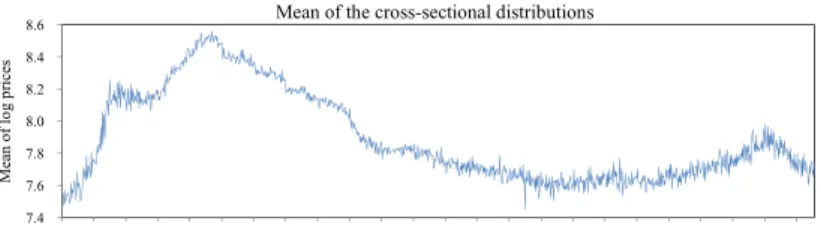
Figure 1: Weekly fluctuations in prices and transaction volume
of their performance.
Figure 1 shows changes in the mean of the cross-sectional house price distribution in the upper panel, the standard deviation in the middle panel, and the transaction volume in the lower panel. We see that the mean price exhibits a sharp increase between the beginning of 1987 and the beginning of 1988. Previous studies refer to this as the first phase of the housing bubble in Tokyo. After a short break in 1988, prices started to rise again in 1989 and continued to rise until the fall of 1990. This is the second phase of the housing bubble. Soon after the fall of 1990, prices started to turn down, followed by a slow but persistent decline for more than a decade until prices bottomed out in 2002, when the mean price reached the level before the bubble started in 1987. Prices finally began to rise again in 2003 and continued to rise until registering a sharp decline in 2008 due to the recent global financial crisis.
Turning to the standard deviation shown in the middle panel, this exhibits a sharp rise during the first phase of the bubble and stayed high during the second phase.3 Finally, the
3We also see a secular increase in price dispersion since 1993. We are not quite sure why this is the case, but recent studies, including Van Nieuwerburgh and Weill (2010) and Gyourko et al. (2006) find some evidence that the recent rise in house price dispersion across regions in the United States is related to the change in income distribution across regions. For example, Van Nieuwerburgh and Weill (2010) find that the cross- sectional coefficient of variation (CV) of house prices across 330 metropolitan statistical areas in the United States increased from 0.15 in 1975 to 0.53 in 2007. Through a counterfactual simulation, they show that this
bottom panel, which shows the transaction volume, indicates that the number of transactions exhibits a sharp increase at the beginning of 1989, exactly when the mean price started to rise, although the transaction volume remained practically unchanged during the first phase of the bubble. Somewhat interestingly, the transaction volume remained at a high level even in 1991 and 1992, when the mean price had already started to decline.
2.2 Empirical strategy
A widely used approach to deal with product heterogeneity in terms of quality is hedonic analysis and there are numerous applications to housing services. The core idea of hedonic analysis is that the value of a product is the sum of the values of product characteristics. For example, Shimizu et al. (2010) start their analysis by assuming that the value of a house is the sum of the values of attributes such as its floor space, its age, the commuting time to the nearest station, and so on, and run hedonic regressions using these attributes as independent variables.
This idea has important implications regarding the shape of the cross-sectional distribution of house prices. To show this, let us start by assuming that the price of house i at a particular point in time, which is denoted by Pi,4 is the sum of K components:
Pi = F (Xi1, Xi2, . . . , Xik, . . . , XiK) (1) where Pi and Xik are both random variables and Xi1, . . . , XiK are assumed to be independent from each other. Furthermore, we assume a multiplicative functional form such that
Pi=
K
∏
k=1
Xik. (2)
Taking logarithm of both sides of this equation leads to:
ln Pi =
K
∑
k=1
xik (3)
where xik ≡ ln Xik. This equation appears frequently in hedonic analyses of house prices. It simply states that the price of a house is equal to the sum of K random variables.
Given this setting, the central limit theorem tells us that the sum of these random variables converges to a normal distribution if the number of attributes, K, goes to infinity. Let us denote the variance of xik by s2k, and define the average variance ¯s2K as
¯ s2K ≡ 1
K (s
2
1+ s22+ · · · + s2K) .
increase in dispersion of house prices is accounted for mostly by the increase in income inequality.
4Note that the subscript for time is dropped here to simplify the exposition.
10-4 10-3 10-2 10-1 100
5 6 7 8 9 10 11
log P
PDF in 2008 Normal
10-4 10-3 10-2 10-1 100
7 7.5 8 8.5 9 9.5 10 10.5 11 11.5
CDF
log P
CDF in 2008 Normal Exponent = 2.8
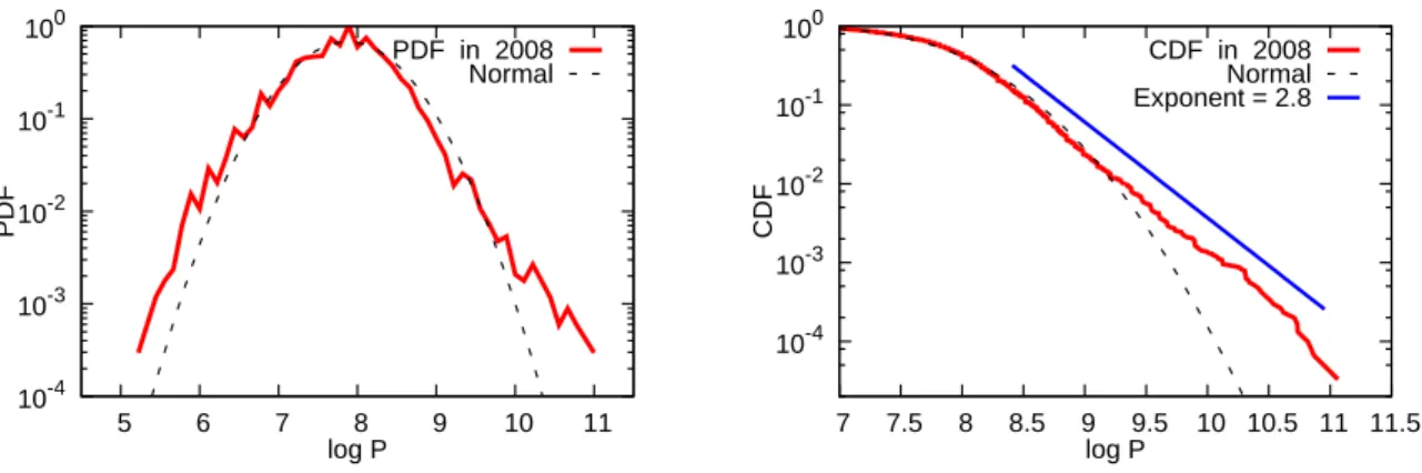
Figure 2: House price distribution in 2008
Then, according to the Lindberg-Feller central limit theorem, the sum of random variables
∑K
k=1xik converges to a normal distribution as K goes to infinity if the average variance ¯s2K converges to a finite constant (namely, limK→∞s¯2K = ¯s2) and the following condition is satisfied:
K→∞lim
maxk≤K{sk}
K ¯sK = 0. (4)
In other words, the theorem states that the sum of random variables, regardless of their form, will tend to be normally distributed. A notable feature of this result is that it does not require that the variables in the sum come from the same underlying distribution. Instead, the theorem requires only that no single term dominates the average variance, as stated in (4). Put differently, condition (4) states that none of the random variables is dominantly large relative to their sum.5 A famous textbook example of the central limit theorem is the distribution of persons’ height. The height distribution of, say, mature men of a certain age can be considered normal, because height can be seen as the sum of many small and independent effects. Similarly, the log price of houses will be normally distributed if house prices are determined as the sum of many small and independent effects.
The above argument suggests that the lognormal distribution can be seen as a benchmark for the cross-sectional distribution of house prices. However, some previous studies on house price distributions find that the actual distributions have fatter tails than a lognormal distri- bution. For example, McMillen (2008), using data on single family houses in Chicago for 1995, shows that the kernel density estimates for the log price are asymmetric, with a much fatter lower tail. Against this background, we examine the extent to which the house price distribu- tion deviates from a lognormal distribution using our observations for 2008. The results are presented in Figure 2, where the left panel shows the probability density function (PDF), with the horizontal axis representing the yen price in logarithm and the vertical axis representing
5For more on this theorem, see Feller (1968). Greene (2003) provides a compact description of various versions of the central limit theorem including this one.
the corresponding density, also in logarithm. The empirical distribution is shown by the red line while the lognormal distribution with the same mean and standard deviation is shown by the black dotted line. The figure indicates that the tails of the empirical distribution are fatter than those of the lognormal distribution. In particular, the upper tail of the empirical distribu- tion is much fatter than that of the lognormal distribution. To examine the differences in the upper tail more closely, we accumulate the densities from the right (upper) tail to produce the cumulative distribution function (CDF), which is shown in the right panel. In this panel, the value on the vertical axis corresponding to the value of 9.2 on the horizontal axis, for example, is 0.01, meaning that the fraction of houses whose prices are equal to or higher than that price level is 1 percent. We now see more clearly that the upper tail of the empirical distribution is fatter than that of the lognormal distribution. For example, the fraction of housing units whose price deviates from the mean by more than 3σ is about 1.47 percent, while the corresponding number for the lognormal distribution is only 0.26 percent.
What causes the empirical distribution to deviate from the benchmark (i.e., the lognormal distribution)? This is the main topic we address in this paper. Our hypothesis is that some of the factors that determine house prices are dominantly volatile, so that condition (4) is violated. Denoting these dominant factors by vector Zi, the house price distribution, Pr(Pi = p), can be decomposed as follows:
Pr(Pi = p) =∑
z
Pr(Pi = p | Zi = z) Pr(Zi= z). (5) Note that the house price distribution conditional on Zi, namely Pr(Pi = p | Zi = z), should be a lognormal distribution, since the dominant factors are now fully controlled for. This means that the right-hand side of equation (5) is a weighted sum of lognormals, with the weights being given by Pr(Zi= z). We know that the sum of lognormals with different means and variances is no longer a lognormal (see, for example, Feller (1968)), and the hypothesis we examine is that this is why the house price distribution deviates from the benchmark. Given this hypothesis, we proceed as follows in the remainder of the paper: we first specify the dominant factors and then eliminate them, thereby constructing prices that are adjusted for these factors; finally, we examine whether these adjusted prices follow a lognormal distribution.
Diewert et al. (2010) argue that there are three important price determining characteristics: the land area of the property; the livable floor space area of the structure; and the location of the property. Similarly, previous studies on house prices in Japan, including Shimizu et al. (2010), find that the floor space of a housing unit (especially in the case of condominiums) and its location play dominantly important roles in determining its price. This empirical evidence suggests that the size and the location of a property are key candidates for the Z variables. We will identify and eliminate the size effect in the next section, and the location effect in Section 4.
10-4 10-3 10-2 10-1 100
-8 -6 -4 -2 0 2 4 6 8
Normalized log P 1986
1987 1988 1989 1990 1991 19921993 Normal
10-5 10-4 10-3 10-2 10-1 100
-1 0 1 2 3 4 5 6 7 8
CDF
Normalized log P 1986 1987 1988 1989 1990 1991 19921993 Normal
10-4 10-3 10-2 10-1 100
-8 -6 -4 -2 0 2 4 6 8
Normalized log P 1994
19951996 1997 1998 1999 2000 2001 Normal
10-5 10-4 10-3 10-2 10-1 100
-1 0 1 2 3 4 5 6 7 8
CDF
Normalized log P 1994 19951996 1997 1998 1999 2000 2001 Normal
10-4 10-3 10-2 10-1 100
-8 -6 -4 -2 0 2 4 6 8
Normalized log P 2002
2003 2004 2005 2006 2007 2008 2009 Normal
10-5 10-4 10-3 10-2 10-1 100
-1 0 1 2 3 4 5 6 7 8
CDF
Normalized log P 2002 2003 2004 2005 2006 2007 2008 2009 Normal
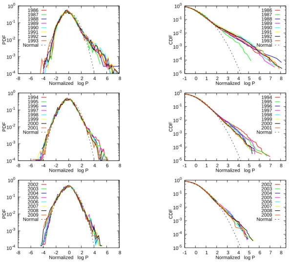
Figure 3: House price distributions by year
3 Size-adjustment to House Prices
3.1 Distribution of unadjusted house prices
Figure 3 presents the PDFs and the CDFs of the cross-sectional price distribution for each year from 1986 to 2009. To make the price distributions in different years comparable, we normalize the log prices in year t by subtracting the mean in year t (i.e., the mean of log prices in year t) and dividing by the standard deviation in year t (i.e., the standard deviation of log prices in year t). The lognormal lines in the figure represent the CDF of a standard lognormal distribution. Note that the CDFs are constructed in the same way as in Figure 2, that is, the value on the vertical axis corresponding to a price level is the sum of the densities above that price level.
The first thing we see from the figure is that, as in Figure 2, the PDFs and the CDFs show fatter upper tails than a lognormal distribution. More importantly, we see that the deviation
from a lognormal distribution tends to be larger in the late 1980s and the first half of the 1990s. Specifically, the PDFs in these years are substantially skewed to the right, indicating that during the bubble period house prices did not rise by the same percentage for every housing unit; instead, price increases were concentrated in particular housing units, so that relative prices across houses changed significantly.
The CDFs in this figure provide more detailed information regarding the shape of the price distributions. We see that the CDF for each year forms an almost straight line in this log- log graph, implying that the house price distribution is well approximated by a power law distribution (or a Pareto distribution) at least in the tail part, the PDF and CDF of which are given by
Pr(Pit= p) = ζtm
ζt
t
pζt+1; Pr(Pit ≥ p) = ( mt
p )ζt
; p > mt> 0 (6) where Pit denotes the price of house i in period t, and ζt and mt are time-variant positive parameters.6 The shape of a power law distribution is mainly determined by the parameter ζt, which is referred to as the exponent of the power law distribution. Smaller values for ζtimply fatter tails. Note that the CDF given in (6) implies that
ln Pr(Pit≥ p) = −ζtln p + ζtln mt.
In other words, the log of the cumulative probability should be linearly related to the log price, and the slope of the linear line between the two variables should be equal to −ζt. The CDFs in Figure 3 suggest the presence of such a linear relationship between the log price and the log of the cumulative probability. We see from the CDF in Figure 2 that ζ2008is about 2.8. Similarly, we find from the corresponding figures for the other years (which are not shown due to space limitations) ζ also all take values of around three. 7
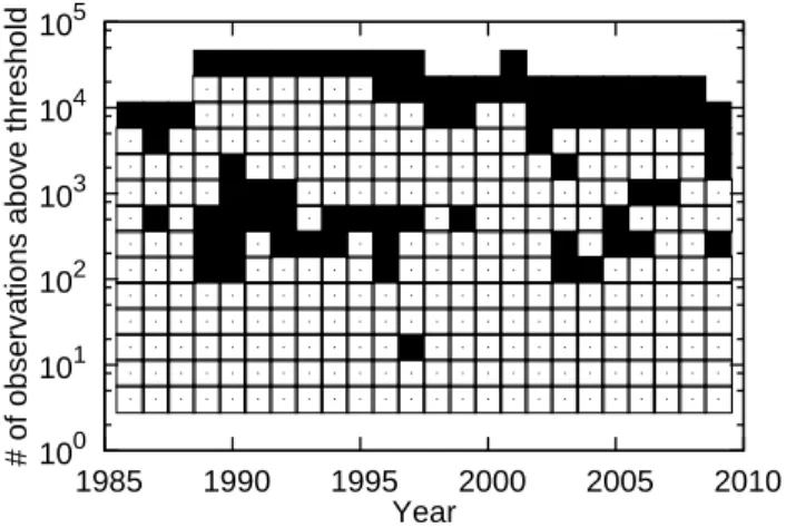
As a goodness-of-fit test, we employ the test proposed by Malevergne et al. (2009). Specif- ically, we test the null hypothesis that, beyond some threshold u, the upper tail of the house price distribution is characterized by a power law distribution
6See Gabaix (2008) for an extensive survey of empirical and theoretical studies on power laws in various economic contexts such as income and wealth, the size of cities and firms, and stock market returns.
7Note that we cannot obtain estimates for ζt from Figure 3. The CDFs in Figure 3 are for normalized prices, which are defined by [Pitexp(−µt)]1/σt, where µt and σt are the mean and the standard deviation in year t. Therefore, the slope of each CDF in Figure 3 is given by σtζt (rather than ζt) if the original price follows the power law distribution given by (6). Taleb (2007) provides many examples of power law distributions. For example, the net worth of Americans follows a power law distribution with an exponent of 1.1; the frequency of the use of words follows such a distribution with an exponent of 1.2; the population of U.S. cities has an exponent of 1.3; the number of hits on websites has an exponent of 1.4; the magnitude of earthquakes has an exponent of 2.8; and market moves have an exponent of 3 (or lower). The exponents for the house price distributions estimated here are greater than most of these figures, implying that the tail part of the house price distributions are less fat than in the other examples of power law distributions.
100 101 102 103 104 105
1985 1990 1995 2000 2005 2010
# of observations above threshold
Year
■ : The null (power law) is rejected at the 1 percent significance level.
□ : The null is not rejected at the 1 percent significance level. Figure 4: Power law distribution versus lognormal distribution
Pr(P = p; α) = α · u
α
pα+1 · 1p≥u
against the alternative that the upper tail follows a lognormal beyond the same threshold, i.e., Pr(P = p; α, β) =[√ π
βexp ( α2
4β ) (
1 − Φ ( α
√2β
))]−1
1 pexp
(−α lnpu− β ln2 up)· 1p≥u
where Φ(·) represents the CDF of a standard normal distribution. Note that this is equivalent to testing the null that the upper tail of the log price follows an exponential distribution against the alternative that it follows a normal distribution. For this transformed test, Del Castillo and Puig (1999) have shown that the clipped empirical coefficient of variation ˆc ≡ min(1, c) provides the uniformly most powerful unbiased test, where c is the empirical coefficient of variation. The result of our goodness-of-fit test is presented in Figure 4, where the horizontal axis represents the year and the vertical axis represents the number of observations above the threshold u. For example, 103 on the vertical axis means that the threshold u is set such that the number of observations above u is 103. A black square indicates that the null is rejected at the 1 percent significance level for a particular year-threshold combination, while a white square indicates that the null is not rejected at the same significance level. The figure shows that a power law distribution provides a good approximation for the 500 most expensive houses, while a lognormal distribution provides a better approximation for the set of less expensive houses.
10-5 10-4 10-3 10-2 10-1 100
50 100 150 200
Pr(>S)
S
exp( – 0.04 S ) 19861987
19881989 19901991 19921993 19941995 1996
10-5 10-4 10-3 10-2 10-1 100
50 100 150 200
Pr(>S)
S
exp( – 0.04 S ) 19971998
19992000 20012002 20032004 20052006 20072008 2009
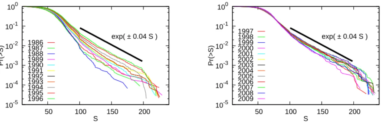
Figure 5: Cumulative house size distributions 3.2 Distribution of house sizes
Previous studies on wealth (or income) distributions across households have typically found that those distributions are characterized by fat upper tails, and that they follow a power law distribution (see Pareto (1896)). Given that houses form an important part of households’ wealth, it may be not that surprising to detect a similar pattern in house price distributions. However, the result that house prices follow a power law distribution is not consistent with the argument based on the central limit theorem. Why do house prices follow a power law distribution rather than a lognormal distribution? As a first step to address this question, we decompose the house price distribution as follows:
Pr(Pit = p) =∑
s
Pr(Pit= p | Si = s) Pr(Si = s), (7) where Sirepresents the size of housing unit i, which is measured by the floor space of that unit. The term Pr(Si = s) represents the distribution of house sizes, while the term∑ Pr(Pit= p | Si = s) represents the distribution of house prices conditional on house size. An important thing to note is that even if each of these conditional distributions is lognormal, the weighted sum of lognormals with different mean and variance is not a lognormal distribution. This is a potential source of the power law tails that we observed in our house price data.
We start by examining the term Pr(Si = s) in equation (7). Figure 5 presents the CDFs of house sizes for each year, with the floor space, measured in square meters, on the horizontal axis and the log of the CDF on the vertical axis. We see that the CDF for each year is close to a straight line in this semi-log graph, implying that the size distribution can be approximated by an exponential distribution whose PDF and CDF are given by
Pr(Si = s) = λtexp (−λts) ; Pr(Si≥ s) = exp (−λts) ; λt> 0. (8) Note that the CDF shown above implies that
ln Pr(Si≥ s) = −λts,
so that the log of the CDF depends linearly on house size. This is what we see in Figure 5. The slope of the CDF line, namely the value of λ, is almost identical for the different years and is somewhere around 0.04.
The fact that house sizes follow an exponential distribution implies that the tails of the size distribution are less fat than those of the price distribution. For example, for 2008, the fraction of housing units whose size deviates from the mean by more than 3σ is only 0.94 percent, while the corresponding number for the price distribution is 1.47 percent.8
3.3 Size-adjusted prices
We now turn to the relationship between the price of a house and its size, which is represented by the conditional probability Pr(Pit = p | Si = s) in equation (7). We propose a hedonic model which is consistent with the fact that house prices and sizes follow, respectively, a power law distribution with an exponent of ζt and an exponential distribution with an exponent of λt. That is, the log prices are determined as
ln Pit∼( λt
ζt )
Si+ ϵit, (9)
where ϵit is a normally distributed random variable, which, as we saw in Section 2.2, can be interpreted as the sum of many small and independent factors. To show equation (9), we first note that the PDF of the exponential distribution given in (8) implies that (λt/ζt)Si follows an exponential distribution with an exponent of ζt if Si itself is an exponential distribution with an exponent of λt. Next, we can show that the sum of the random variable that follows an exponential distribution and the random variable that follows a normal distribution is well approximated only by the exponential distribution when the sum takes large values (because of the much fatter tails of an exponential distribution).9 Combining the two, the right-hand side of (9) is well approximated by an exponential distribution with an exponent of ζt when the sum of the two terms on the right-hand side takes large values. On the other hand, the fact that Pit follows a power law distribution with an exponent of ζtimplies that ln Pit follows an exponential distribution with an exponent of ζt. In this way we can confirm that each side of equation (9) follows an identical distribution with an identical exponent.10
8To see why the tails of the house size distribution are less fat than the tails of the price distribution, consider a simple example in which household A has 100 times as much wealth as household B, so that A spends 100 times as much money on a house as B. What does A’s house look like? Does it have a bathroom that is 100 times larger than the one in B’s house? Alternatively, does it have 100 bathrooms? Needless to say, neither is true, because even a person of A’s wealth would have little use for such a gigantic bathroom (or so many bathrooms). Instead, it is more likely that the size of A’s house (and therefore the size and/or number of its bathroom) is only, say, 10 times greater and, consequently, the unit area price of A’s house, 10 times higher than B’s.
9See the appendix for a formal proof of this.
10The price-size relationship described by equation (9) provides an answer to the question regarding the choice of functional form for hedonic price equations, which has been extensively discussed by previous studies such
103 104 105
50 100 150 200 250
P
S exp( 0.013 S )
19861987 19881989 19901991 19921993 19941995 1996
103 104 105
50 100 150 200 250
P
S exp( 0.013 S )
19971998 19992000 20012002 20032004 20052006 20072008 2009
25 50 100 200 400
50 100 150 200 250
P / S
S
19861987 19881989 19901991 19921993 19941995
1996 25
50 100 200 400
50 100 150 200 250
P / S
S
19971998 19992000 20012002 20032004 20052006 20072008 2009
Figure 6: Relationship between house size and price
To empirically test the hedonic model given by (9), we first examine for a linear relationship between the log price of houses and their size. The upper panels of Figure 6 show the floor space on the horizontal axis and the median of the log price corresponding to that size on the vertical axis. These panels indicate that there exists a stable linear relationship between the two variables. Furthermore, equation (9) implies that the per unit area price, P/S = [exp(λ/ζ)S + positive constant]/S, decreases with S when S is small and increases with S when S is sufficiently large, so that there should exist a U-shaped relationship between the per unit area price and the house size. The lower panels of Figure 6, in which the vertical axis now measures P/S, confirms this prediction.
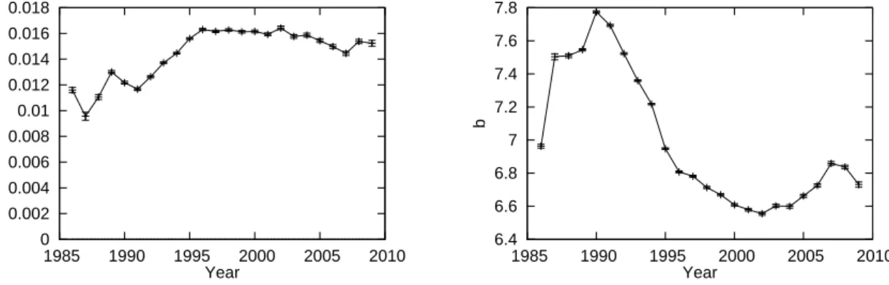
Second, we run an OLS regression of the form
ln Pit= atSi+ bt+ ηit (10)
to see whether the disturbance term ηit is indeed normally distributed as assumed in (9). The regression results are presented in Figures 7 and 8. Figure 7 shows the estimates of a and b for each year. The estimate of a is almost identical across years and is around 0.013, implying that an increase in the house size by a square meter leads to a 1.3 percent increase in the house price. More importantly, the estimate of a is very close to the value predicted by (9). That is, the value of ζ is around 3 as we saw in Section 3.1, and the value of λ is about 0.04 as
as Cropper et al. (1988), Diewert (2003), and Triplett (2004). The novelty of our approach is that we derive this functional form not from economic theories but from the statistical fact that house prices and sizes follow a power law and an exponential distribution, respectively.
0 0.002 0.004 0.006 0.008 0.01 0.012 0.014 0.016 0.018
1985 1990 1995 2000 2005 2010
a
Year
6.4 6.6 6.8 7 7.2 7.4 7.6 7.8
1985 1990 1995 2000 2005 2010
b
Year
Figure 7: Price-size regressions
we saw in Section 3.2, so that the coefficient on Si, namely λ/ζ, should be something around 0.013 (= 0.04/3). This is quite close to the point estimate of a for each year.11 Turning to the estimate of b, this exhibits substantial fluctuations: it increases by more than 20 percent per year from 1986 to 1990 and then declines by 10 percent per year from 1990 to 2002.
Figure 8 shows the CDFs of size adjusted prices defined by P˜it≡[Pitexp(−ˆatSi− ˆbt)]
1/ˆσt
, (11)
where ˆatand ˆbtare the estimates of atand bt, and ˆσt is the estimate for the standard deviation of ηit. Note that the hedonic model given by (9) implies that ˜Pit should be a lognormal distribution. The CDFs of the size adjusted prices are shown in the three panels on the right- hand side of Figure 8, while the price distributions without size adjustments (the same figures as in Figure 3) are shown on the left-hand side. Comparing these two sets of CDFs, we see that the CDFs of the size-adjusted prices are much closer to the CDF of a lognormal distribution. More specifically, the CDFs for 2002 to 2009, which are shown in the lower right panel, are almost identical to the CDF of a lognormal distribution. The same applies to the CDFs for 1996 to 2001, which are shown in the middle right panel. However, the CDFs for 1986 to 1995, which are presented in the upper right and the middle right panels, are still far from the CDF of a lognormal distribution, although they are slightly closer to it than the CDFs of the non-adjusted prices.
4 Location Adjustment to House Prices
The analysis in the previous section suggested that size-adjusted prices followed a lognormal distribution at least for quiet periods without large price fluctuations. This is consistent with
11Note that the per unit area price, exp(aS + b)/S takes its minimum value when S is equal to 1/a. Given the estimate of a, this implies that the per unit area price takes its minimum value when S = 1/0.013 ≈ 75, which is consistent with what we see in the lower two panels of Figure 6.
10-5 10-4 10-3 10-2 10-1 100
-1 0 1 2 3 4 5 6 7 8
CDF
Normalized log P 1986 1987 1988 1989 1990 1991 19921993 Normal
10-5 10-4 10-3 10-2 10-1 100
-1 0 1 2 3 4 5 6 7 8
CDF
Normalized log P – aS 1986 1987 1988 1989 1990 1991 19921993 Normal
10-5 10-4 10-3 10-2 10-1 100
-1 0 1 2 3 4 5 6 7 8
CDF
Normalized log P 1994 19951996 1997 1998 1999 2000 2001 Normal
10-5 10-4 10-3 10-2 10-1 100
-1 0 1 2 3 4 5 6 7 8
CDF
Normalized log P – aS 1994 19951996 1997 1998 1999 2000 2001 Normal
10-5 10-4 10-3 10-2 10-1 100
-1 0 1 2 3 4 5 6 7 8
CDF
Normalized log P 2002 2003 2004 2005 2006 2007 2008 2009 Normal
10-5 10-4 10-3 10-2 10-1 100
-1 0 1 2 3 4 5 6 7 8
CDF
Normalized log P – aS 2002 2003 2004 2005 2006 2007 2008 2009 Normal
Figure 8: Cumulative distributions of size-adjusted house prices
the idea that, as stated in (7), the power law tails of the original prices stem from the mixture of lognormal distributions with different mean and variance. At the same time, the analysis in the previous section showed that the fat tails of the price distribution remain largely unchanged for the bubble period (i.e., the late 1980s and the first half of the 1990s) even after controlling for the size effect. This suggests that there still remains some mixture of lognormal distributions. In this section, we test the hypothesis that the power law tails of the size adjusted prices during the bubble period arise due to the mixture of different lognormal distributions corre- sponding to different regions. To do so, we start by decomposing the size-adjusted price into the sum of conditional distributions:
Pr( ˜Pirt= p)=∑
θ
Pr( ˜Pirt= p | θrt= θ)Pr(θrt= θ) (12)
where ˜Pirt denotes the size-adjusted price for a house located in region r, which is defined by
10-3 10-2 10-1 100
0 0.01 0.02 0.03 0.04 0.05 0.06
CDF
a
1986 19871988 19891990 19911992 1993
10-3 10-2 10-1 100
-1 0 1 2 3 4
CDF
Normalized log P – aS 1986 19871988 19891990 19911992 1993
10-3 10-2 10-1 100
0.2 0.4 0.6 0.8 1 1.2
CDF
SD of Normalized log P – aS 1986 19871988 19891990 19911992 1993
10-3 10-2 10-1 100
0 0.01 0.02 0.03 0.04 0.05 0.06
CDF
a
1994 19951996 19971998 1999 20002001
10-3 10-2 10-1 100
-1 0 1 2 3 4
CDF
Normalized log P – aS 1994 19951996 19971998 1999 20002001
10-3 10-2 10-1 100
0.2 0.4 0.6 0.8 1 1.2
CDF
SD of Normalized log P – aS 1994 19951996 19971998 1999 20002001
10-3 10-2 10-1 100
0 0.01 0.02 0.03 0.04 0.05 0.06
CDF
a
2002 20032004 2005 20062007 20082009
10-3 10-2 10-1 100
-1 0 1 2 3 4
CDF
Normalized log P – aS 2002 20032004 2005 20062007 20082009
10-3 10-2 10-1 100
0.2 0.4 0.6 0.8 1 1.2
CDF
SD of Normalized log P – aS 2002 20032004 2005 20062007 20082009
Figure 9: Dispersion of ar, br and σr across pixels P˜irt≡ Pirtexp(−artSir − brt). The vector of parameters θrt is defined by
θrt≡ (art, brt, σrt), (13)
where the parameters art, brt, and σrtare the coefficient on the house size variable, the constant term, and the standard deviation of the disturbance term in equation (10), but it is assumed in this section that they could differ depending on the location of a house. The location effect is fully controlled for in the conditional distributions Pr( ˜Pirt = p | θrt = θ), so that they should be lognormals. According to equation (12), the distribution of ˜Pirtis a mixture of these lognormals, each of which is for a different region.
We first examine the distribution of θrt across different regions. Specifically, we divide the Greater Tokyo Area into pixels of 0.033 degrees latitude and 0.033 degrees longitude or roughly 3.3 by 3.3 km.12 Then, using size-adjusted prices within a pixel, we run a regression of the form:
ln Pirt= artSir+ brt+ ηirt (14) for each combination of r and t and obtain ˆθrt ≡ (ˆart, ˆbrt, ˆσrt). The regression results are
12Note that one degree is approximately 100 km.
10-5 10-4 10-3 10-2 10-1 100
-2 0 2 4 6 8
CDF
Normalized log(Price) – aS 1986 ds=0.033
ds=0.262 ds=0.524 ds=4.19 Normal
10-5 10-4 10-3 10-2 10-1 100
-2 0 2 4 6 8
CDF
Normalized log(Price) – aS 1998 ds=0.033
ds=0.262 ds=0.524 ds=4.19 Normal
10-5 10-4 10-3 10-2 10-1 100
-2 0 2 4 6 8
CDF
Normalized log(Price) – aS 1990 ds=0.033
ds=0.262 ds=0.524 ds=4.19 Normal
10-5 10-4 10-3 10-2 10-1 100
-2 0 2 4 6 8
CDF
Normalized log(Price) – aS 2002 ds=0.033
ds=0.262 ds=0.524 ds=4.19 Normal
10-5 10-4 10-3 10-2 10-1 100
-2 0 2 4 6 8
CDF
Normalized log(Price) – aS 1994 ds=0.033
ds=0.262 ds=0.524 ds=4.19 Normal
10-5 10-4 10-3 10-2 10-1 100
-2 0 2 4 6 8
CDF
Normalized log(Price) – aS 2006 ds=0.033
ds=0.262 ds=0.524 ds=4.19 Normal
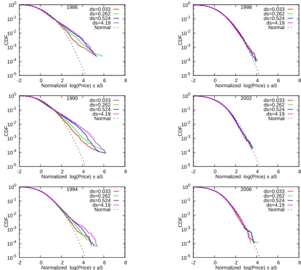
Figure 10: Cumulative distributions of size-adjusted house prices for different pixel sizes
presented in Figure 9.13 The three left-most panels show the CDFs of ˆart, while the panels in the middle and the right-most panels respectively show the CDFs of ˆbrt and ˆσrt. The CDFs of ˆ
artindicate that a is less dispersed across pixels during the period of the bubble and its collapse (1987-1995) than in the other years. On the other hand, the CDFs of ˆbrt and ˆσrt show that these parameters are more highly dispersed during the same period, implying that the sharp price hike during the bubble period was concentrated in particular pixels. Put differently, the housing market was segmented during this period.
Next, we investigate whether the conditional distributions are close to a lognormal distri- bution. Using the estimates of θrtobtained from the regression, we calculate the size-adjusted prices for each pixel:
P˜irt≡[Pirtexp(−ˆartSir− ˆbrt)]1/ˆσrt. (15)
13In conducting these regressions, we use only those pixels with more than twenty transactions in a year. The number of pixels used in the regressions is about 300 for each year.
The estimated CDFs of ˜Pirt are presented in Figure 10 for the years 1986, 1990, 1994, 1998, 2002, and 2006. Note that each of the six panels contains four different lines, each of which corresponds to a different pixel size, namely 4.190 by 4.190 degrees, 0.524 by 0.524 degrees, 0.263 by 0.263 degrees, and 0.033 by 0.033 degrees. The results for 1998, 2002, and 2006 indicate that the CDFs are very close to a lognormal distribution, irrespective of pixel size. This is not very surprising given that, as we saw in the previous section, the CDFs in these years were already close to a lognormal distribution before controlling for the location effect. For the period of the bubble and its collapse, we see more interesting results: for 1986, 1990, and 1994, the estimated CDF tends to become closer to a lognormal distribution as the pixel size becomes smaller.14
In sum, the analysis in this section shows that the distribution of size-adjusted prices within a pixel is fairly close to a lognormal distribution even during the period of the bubble and its collapse, but its mean and standard deviation are highly dispersed across different pixels. As a result, the sum of these lognormals turns out to be far from a lognormal distribution during this period. In other words, heterogeneity across pixels in terms of mean and standard deviation is the source of the fat upper tail of the size-adjusted price distribution during the period of the bubble and its collapse.
5 Summary and Some Policy Implications
In this paper, we found that the cross-sectional distribution of house prices in the Greater Tokyo Area has a fat upper tail, and the tail part is close to that of a power law distribution. On the other hand, the cross-sectional distribution of house sizes measured in terms of floor space has less fat tails than the price distribution and is close to an exponential distribution. We proposed a hedonic model consistent with these findings and confirmed that size-adjusted prices follow a lognormal distribution except for the period of the asset bubble and its collapse in Tokyo for which the price distribution remains asymmetric and skewed to the right even after controlling for the size effect. As for the period of the bubble and its collapse, we found some evidence that the sharp price movements were concentrated in particular areas, and this spatial heterogeneity is the source of the fat upper tail.
The analysis in this paper shows that the cross-sectional distribution of size-adjusted prices is very close to a lognormal distribution during regular times but deviated substantially from a lognormal during the bubble period. This suggests that the shape of the size-adjusted price distribution, especially the shape of the tail part, may contain information useful for the de-
14It should be noted that the estimated CDF does not fully converge to a lognormal even in the case of the smallest pixels. It may be the case that the CDF becomes much closer still to a lognormal distribution if we were able to reduce the pixel size even further. Unfortunately, we cannot do so because of the limited number of observations.
tection of housing bubbles. That is, the presence of a bubble can be safely ruled out if recent price observations are found to follow a lognormal distribution. On the other hand, if there are many outliers, especially near the upper tail, this may indicate the presence of a bubble, since such price observations are very unlikely to occur if they follow a lognormal distribution. This method of identifying bubbles is quite different from conventional ones based on aggregate measures of housing prices, which are estimated either by hedonic or repeat-sales regressions, and therefore should be a useful tool to supplement existing methods.
References
[1] Cochrane, J. H. (2002), “Stocks as Money: Convenience Yield and the Tech-Stock Bubble,” NBER Working Paper 8987.
[2] Cropper, M. L., L. B. Deck, and K. E. McConnell (1988), “On the Choice of Functional Form for Hedonic Price Functions,” Review of Economics and Statistics 70(4): 668-675. [3] Del Castillo, J., and P. Puig (1999), “The Best Test of Exponentiality Against Singly
Truncated Normal Alternatives,” Journal of the American Statistical Association 94, 529- 532.
[4] Diewert, W. E. (2003), “Hedonic Regressions: A Consumer Theory Approach,” in R. C. Feenstra and M. D. Shapiro (eds.), Scanner Data and Price Indexes, National Bureau of Economic Research Studies in Income and Wealth, Vol. 64, Chicago, IL: University of Chicago Press, 317-48.
[5] Diewert, W. E., J. de Haan, and R. Hendriks (2010), “The Decomposition of a House Price Index into Land and Structures Components: A Hedonic Regression Approach,” Discussion Paper 10-01, University of British Columbia.
[6] Feller, W. (1968), An Introduction to Probability Theory and Its Applications. Vol. 1, Third Edition, New York: Wiley.
[7] Gabaix, X. (2008), “Power Laws in Economics and Finance,” NBER Working Paper 14299. [8] Green, W. (2003), Econometric Analysis, Fifth Edition, Upper Saddle River, NJ: Prentice
Hall.
[9] Gyourko, J., C. Mayer, and T. Sinai (2006), “Superstar Cities,” NBER Working Paper 12355.
[10] Maattanen, N., and M. Tervio (2010), “Income Distribution and Housing Prices: An Assignment Model Approach,” CEPR Discussion Paper 7945.
[11] Malevergne, Y., V. Pisarenko, and D. Sornette (2009), “Gibrat’s Law for Cities: Uniformly Most Powerful Unbiased Test of the Pareto against the Lognormal,” American Economic Review, forthcoming.
[12] McMillen, D. P. (2008), “Changes in the Distribution of House Prices over Time: Struc- tural Characteristics, Neighborhood, or Coefficients?” Journal of Urban Economics 64(3): 573-589.
[13] Shimizu, C., K. G. Nishimura, and Y. Asami (2004), “Search and Vacancy Costs in the Tokyo Housing Market: An Attempt to Measure Social Costs of Imperfect Information,” Review of Urban and Regional Development Studies 16(3): 210-230.
[14] Shimizu, C., K. G. Nishimura, and T. Watanabe (2010), “House Prices in Tokyo: A Comparison of Repeat-Sales and Hedonic Measures,” Research Center for Price Dynamics Discussion Paper 62, Hitotsubashi University.
[15] Taleb, N. N. (2007), The Black Swan: The Impact of the Highly Improbable, New York: Random House, Inc.
[16] Triplett, J. (2004), “Handbook on Hedonic Indexes and Quality Adjustments in Price Indexes: Special Application to Information Technology Products,” OECD Science, Tech- nology and Industry Working Papers 2004/9.
[17] Van Nieuwerburgh, S., and P. O. Weill (2010), “Why Has House Price Dispersion Gone Up?” Review of Economic Studies, forthcoming.