本文 Thesis 総合研究大学院大学学術情報リポジトリ A1744本文

Growth History of Galaxy Clusters

Traced by Protoclusters at _{z ∼ 3 − 6}

Thesis for the degree of Doctor of Science

Jun Toshikawa

Department of Astronomical Science

School of Physical Science

The Graduate University for Advanced Studies

February 25, 2015

ACKNOWLEDGMENTS

First and foremost, I would like to express my deep sense of gratitude to my supervisor, Associate Prof. Nobunari Kashikawa. I could ask him for advice whenever I was in trouble, and he gave me uncountable instruction. Furthermore, he started to teach me even before my entering the graduate university. I could learn many things about the research of astronomy. This thesis would not have been possible unless his support. I am also thankful for the excellent example, he has provided as a successful man both in research and home.

I would like to appreciate Dr. Kazuaki Ota. Thanks to his previous work, I could get my research off to a very good start. He supported my research by giving suggestion as well as data. When I addressed a paper or proposals, he carefully checked them like a referee and provided valuable comments. It is an honor for me to take over his work, and I would like to make further advance.

I would like to show my deep appreciation for Prof. Roderik Overzier. With his great help from theoretical aspects, we were able to push our research toward new directions. Theoretical part of this thesis could not be completed without his supports. I have a lot of respect for his versatility from observational to theoretical research.

I am indebted to my collaborators for providing data, instruction, and comments on my study. Assistant Prof. Tomoki Morokuma provided optical imaging data; Associate Prof. Motohara Kentaro and Dr. Masao Hayashi provided near-infrared imgaging data; Associate Prof. Eiichi Egami provided mid-infrared imaging data. In addition to imaging data, Associate Prof. Kazuhiro Shimasaku, Associate Prof. Tohru Nagao, and Dr. Linhua Jiang brought me spectroscopic data. Dr. Takashi Hattori kindly gave me a lot of help for observations and data analysis, and Dr. Masao Hayashi kindly taught me how to do and gave me useful codes. Thanks to their instruction, I could save time and concentrate on interpretation and discussion. When I had to express my idea or interpretation in a paper or proposals, Prof. Matthew A. Malkan closely checked my English and corrected it to be more impressive. This thesis is constructed from these observational data, and I could not have researched without their cooperation.

I am also grateful to my colleagues, Dr. Takatoshi Shibuya, Mr. Yoshifumi Ishizaki, Mr. Shogo Ishikawa, and Mr. Masafusa Onoue for discussion at the seminar and a lot of help with my study. They empathetically taught me many technical things and answered even my petty questions. Not only about research, they answered my questions about the life in National Astronomical Observatory of Japan or in Tokyo. Therefore, I could get used to new surroundings soon and enjoy my Ph.D. course. On top of that I could get many help from Associate Prof. Tadayuki Kodama, Dr. Masakazu Kobayashi, Dr. Yousuke Utsumi, and Dr. Ken-ichi Tadaki.

I acknowledge financial support from the Japan Society for the Promotion of Science (JSPS) through JSPS Research Fellowship for Young Scientists for that last three years of the doctor course. I have been able to spend all time for my research due to the support.

Finally, I would like to thank to my parents and my wife for their understanding and encouragement. Because they are supporting my life in every way, I can go ahead.

ABSTRACT

ABSTRACT

We performed a systematic survey of protoclusters of galaxies across cosmic time (z ∼ 3 − 6). Protoclusters, which are defined as overdense regions of galaxies in the high-redshift universe, are the precursors of massive clusters of galaxies in the local universe. In the uni- verse at present, the spatial distribution of galaxies is significantly inhomogeneous. This is termed the large-scale structure, and galaxies reside in various environments from clusters to voids; it is clear that the physical properties of galaxies differ depending on their environment. Clusters of galaxies occupy particularly high-density regions in the large-scale structure of the universe, although the universe was initially almost homogeneous. The environments of clusters evolved drastically from the small density fluctuations of dark matter via merging and accre- tion. Therefore, galaxy clusters are important targets for understanding both galaxy evolution and structure formation. However, the number of known protoclusters is limited, and such structures are particularly rare. Increasing the number of known high-redshift protoclusters is the first step to improving our understanding of the entire history of cluster formation as well as the significance of environmental effects on galaxy evolution. Furthermore, most of the known protoclusters were discovered by using the probe of overdense regions, such as radio galaxies (RGs) and quasars (QSOs), which lie in very massive halos in the local universe. Some contradictory results, including that RGs and QSOs reside in low-density regions, have been observed at high redshift. Systematic searches for protoclusters without RGs or QSOs are im- perative to create unbiased samples and to lead correct understanding of cluster growth. In this thesis, we have probed for protoclusters from z ∼ 6 to z ∼ 3 with wide-field imaging, not using RGs/QSOs, in order to discover rare objects in high-redshift universe.

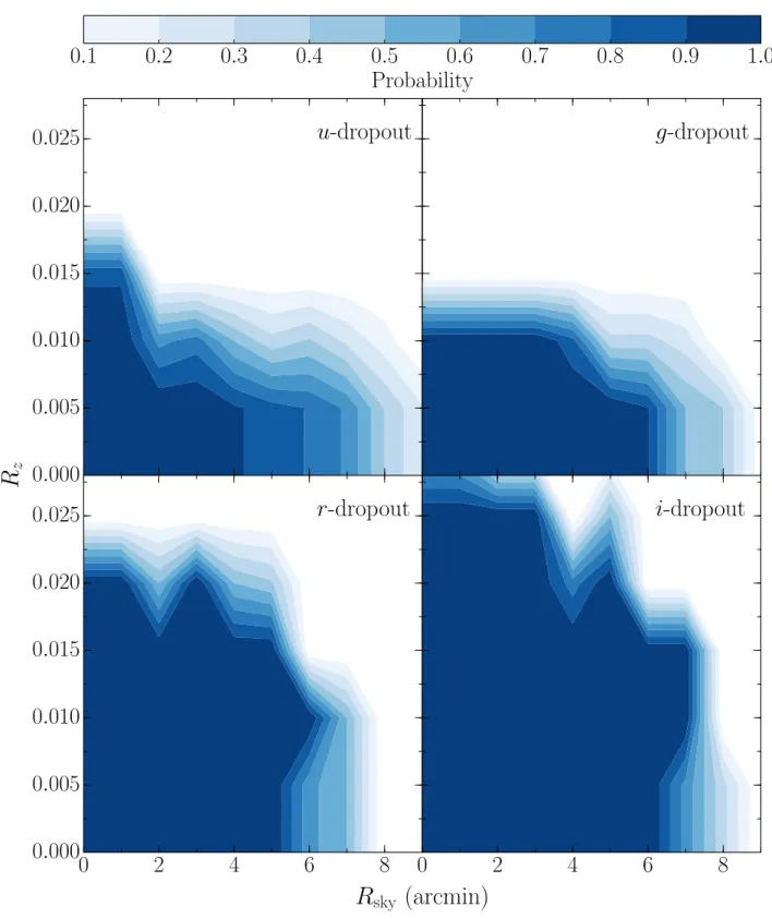
We used two sets of wide-field imaging data from the Subaru Deep Field and (SDF) and the Canada-France-Hawaii Telescope Legacy Survey (CFHTLS) Deep Fields. Both datasets are unique in terms of survey depth and area, which is advantageous in finding rare objects in the high-redshift universe. Based on samples selected using a dropout technique, we derived the sky distribution of galaxies from z ∼ 6 to z ∼ 3. In total, 22 protocluster candidates were identified from z ∼ 3 to z ∼ 6, based on surface overdensity defined by counting galaxies within a fixed aperture. We applied the same overdensity measurement to the simulated galaxy sample, which was selected to have the same redshift distribution from the light-cone model as in the dropout sample. We find that the overdensity at high redshift is strongly correlated with the descendant halo mass at z = 0, and ≳ 85% of the overdense regions with significance greater than 4σ are expected to grow up to dark matter halos with M > 10¹⁴M⊙, which corresponds to nearby rich cluster of galaxies, at z = 0. The number density of detected protocluster candidates with an overdense significance of > 4σ is approximately one candidate per 1 deg², which is consistent with the prediction of the model. The distribution of protocluster members is expected to be within 2 physical Mpc radius on sky, as well as the line-of-sight velocity of

∆v < 1000 km s⁻¹. Spectroscopic observations were carried out for nine of these candidates, and four genuine protoclusters were discovered by confirming galaxy clustering in spatial and line-of-sight directions. According to the redshifts determined by detecting the Lyα emission lines, we distinguished protocluster members from non-members. Furthermore, we discovered a protocluster at z = 6.01, which is the highest-redshift protocluster ever found.

Based on the protocluster sample, we investigated protocluster structure and galaxy prop- erties. We find that a protocluster at z = 6.01, which is far from virialization, is composed of

several small galaxy pairs. In contrast, at z = 3.67, half of the protocluster galaxies are con- centrated in the small central region of a protocluster, and the others are distributed around it. This result suggests that protocluster structure evolves drastically toward a virialized structure from z ∼ 6 to z ∼ 4, although more protocluster samples are required to confirm a general trend.

We investigated differences in the properties of protocluster and field galaxies. There are no significant differences in MUV, LLyα, and EWrest at z = 6.01; however, the Lyα emission lines are significantly suppressed in a z = 3.67 protocluster compared to field galaxies at the same redshift. We consider two possible causes of this difference: attenuation due to dust in member galaxies (which is associated with the rapid evolution of galaxies in high- density environments), and absorption due to intracluster neutral hydrogen gas. We were not able to find differences in UV continuum slope (an indicator of dust) between protocluster and field galaxies. A large amount of neutral hydrogen gas may explain the suppression of Lyα emission lines in protocluster galaxies; however, this hypothesis currently lacks significant supporting evidence. Our finding of Lyα suppression in more dynamically mature protocluster at lower redshift suggests that the properties of protocluster galaxies might be affected by their environment in combination with dramatic changes in the internal structure. However, we find two z ∼ 3 protoclusters that exhibit inconsistent tendencies in the protocluster properties even at the same redshift. This study, as a precursor to the Hyper Suprime-Cam (HSC) survey, demonstrates that wide-field imaging is an effective tool to locate high-redshift protoclusters, and future HSC surveys will enable us to derive a more complete picture of cluster formation and galaxy evolution in high-density environments.

CONTENTS

CONTENTS

ACKNOWLEDGMENTS i

ABSTRACT ii

1 INTRODUCTION 1

1.1 Mature Clusters of Galaxies . . . 1

1.2 Forming Clusters: Protoclusters . . . 3

1.3 This Thesis . . . 6

2 SAMPLE SELECTION 8 2.1 Photometric Data . . . 8

2.1.1 Subaru Deep Field . . . 8

2.1.2 CFHTLS Deep Fields . . . 8

2.2 Source Detection and Photometry . . . 15

2.3 Selection Criteria of Lyman Break Galaxies . . . 18

3 PROTOCLUSTER CANDIDATES 24 3.1 Sky Distribution and Overdensity . . . 24

3.2 Comparison with Model Predictions . . . 32

4 FOLLOW-UP SPECTROSCOPY 37 4.1 How to Confirm Protocluster . . . 37

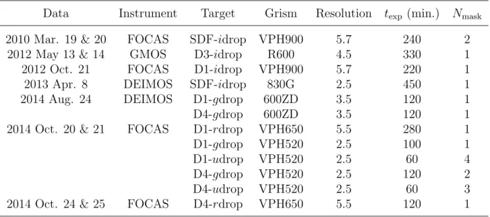
4.2 Observations . . . 39

4.3 Line Contaminations . . . 41

4.4 Results . . . 42

5 SED FITTING 78 5.1 Method . . . 78

5.2 Results . . . 79

6 DISCUSSIONS 82 6.1 Protocluster Search in Blank Fields . . . 82

6.2 Protocluster Structure . . . 83

6.2.1 z = 6.01 protocluster in the SDF . . . 83

6.2.2 z = 3.67 protocluster in the CFHTLS D4 . . . 85

6.3 Properties of Protocluster Members . . . 92

6.3.1 z = 6.01 Protocluster in the SDF . . . 92

6.3.2 z = 3.67 Protocluster in the CFHTLS D4 . . . 93

6.3.3 z ∼ 3 Protocluster in the CFHTLS D1 and D4 . . . 95

7 CONCLUSION 101

REFERENCES 103

1. INTRODUCTION

1. INTRODUCTION

1.1. Mature Clusters of Galaxies

The present-day universe exhibits the large-scale structures composed of clusters, filaments, voids, and sheet-like structures. The spatial distribution of galaxies is significantly inhomoge- neous, and clusters of galaxies (typically containing between 50 and 10³ member galaxies) are frequently located at the intersections of filaments. These rich structures are surrounded by extremely underdense regions, termed “voids,” which contain no (or very few) galaxies. The large-scale structure was first discovered from the angular distribution of galaxies based on photographic maps (Seldner et al. 1977). Subsequently, many of the early galaxy surveys, such as the CfA Redshift Survey (de Lapparent et al. 1986), more clearly revealed the structures of the distribution of galaxies. Modern galaxy redshift surveys, such as the Two-degree Field Galaxy Redshift Survey (2dFGRS; Colless et al. 2001), the Sloan Digital Sky Survey (SDSS; e.g., Tegmark et al. 2004), and the Galaxy And Mass Assembly (GAMA; Driver et al. 2011), revealed a more obvious filamentary structure, and showed that clusters form large networks of galaxies, termed the “cosmic web,” connected by groups of galaxies or filaments (e.g., Smargon et al. 2012; Einasto et al. 2014). From these observations, we recognized that galaxies reside in various environments from clusters to voids in the local universe. At the beginning of the universe, however, the amplitude of the density fluctuations was small. Exploring the structure formation toward the early universe has been one of the hottest issues in astronomy in recent years. Our understanding of large-scale structure have been aided by sophisticated simulations (e.g., Arag´on-Calvo et al. 2010; Angulo et al. 2012; Park et al. 2012). Based on the cold dark matter (CDM) models, the density fluctuations of dark matter evolve as time progress by merg- ing and by accretion. Baryonic matter accumulates in the gravitational potential wells formed by the dark matter (Springel et al. 2005). Particularly dense matter fluctuations eventually re- sulted in the formation of galaxies and clusters. Clusters of galaxies, which occupy the densest parts of the large-scale structure of the local universe, have evolved considerably compared to the initial condition of the universe. In principle, we can derive the information on the early universe from observations of the local universe, if the universe evolved under the simple laws of physics. However, due to poorly understood complex physical processes, information derived only from the local universe cannot be used to draw strong conclusions about the evolution of the universe. More reliable results may be obtained from both direct observations of the high- redshift universe and the local universe. Therefore, the growth of density fluctuations measured from comparisons of abundances and mass distributions of present-day clusters with those at earlier times provides unique constraints on the ΛCDM concordance model (e.g., Vikhlinin et al. 2003; Voit 2005; Mortonson et al. 2011).

Clusters of galaxies are of significant astronomical interest in terms of the environmental dependence of galaxy evolution. Observations of the local universe have revealed that the fraction of elliptical galaxies is larger in higher density region; this is known as the “morphology- density relation” (e.g., Dressler 1980). Moreover, clusters of galaxies represent a distinct relationship in the color-magnitude diagram. The “red sequence” of clusters is mainly composed of spheroidal and lenticular galaxies with old stellar populations and high stellar masses (e.g., Visvanathan & Sandage 1977; Lerchster et al. 2011). Bright and red (i.e., massive and old) galaxies are likely to inhabit clusters of galaxies, and the shape of the stellar mass function

is strongly influenced by the environment (e.g., Vulcani et al. 2012). Even in modest galaxy group environments, the star formation is known to be effectively quenched at z < 0.1 (e.g., Rasmussen et al. 2012). Furthermore, local clusters sometimes harbour cD galaxies, which are more massive, more extended, and less dense than the normal elliptical galaxies. In particular, massive and bright elliptical galaxies in a cluster have significantly different properties from their field counterparts, such as a larger stellar velocity dispersion and a higher α/Fe ratio. These differences suggest that elliptical galaxies in a cluster contain more dark matter and are characterized by a shorter star-formation timescale (Thomas et al. 2005; von der Linden et al. 2007). These are intuitively expected within the hierarchical structure formation scenario: halos in higher-density regions are expected to collapse earlier and merge more rapidly, leading to earlier galaxy formation and more rapid evolution (Kauffmann et al. 1999; Benson et al. 2001; Springel et al. 2005; De Lucia et al. 2006). In this manner, both observational and theoretical studies predict that galaxy evolution strongly depends on the environment. When and how did these distinct properties form? Galaxy evolution is determined by diverse physical processes, which are closely interrelated. What is the most dominant process in the evolutionary history of galaxy: when or where galaxies are born? Even if galaxies in high- and low-density environments have the same evolutionary history, environmental differences between cluster and field galaxies as seen in the present universe could be caused simply because cluster galaxies are formed earlier. In contrast, it is likely that galaxies follow different growth paths due to posteriori effects following their birth; this would also be an origin of the diversity of the properties of galaxies. In high-density regions, many physical processes, such as galaxy mergers and interactions, would affect the evolutionary history. Highly evolved clusters in the local universe have been intricately affected by both these nature and nurture physical processes; thus, it is difficult to sort out which factors are more essential in our understanding of cluster and galaxy evolution. One promising approach is to directly investigate the primitive properties of galaxies in the first clusters of galaxies to appear during the early epoch.

As described above, clusters of galaxies are important targets in terms of both structure formation and galaxy evolution. The number density of clusters in the local universe is typically 10⁻⁶ − 10⁻⁷Mpc⁻³, although it depends on the richness of the cluster, as well as the number density of groups or poor clusters is 10⁻⁴ − 10⁻⁶Mpc⁻³ (Bahcall & Cen 1993). Clusters of galaxies are defined as being in dynamical equilibrium, and the deep gravitational wells contain the bulk of the very hot gases (T ≥ 10⁷K). As a result, clusters of galaxies are detected most readily from X-ray emissions (e.g., Rosati et al. 1998), or by the effects on the cosmic microwave background (e.g., Sunyaev & Zeldovich 1972; Barbosa et al. 1996); most known clusters of galaxies have been discovered during astronomical X-ray surveys (e.g., B¨ohringer et al. 2004; Lloyd-Davies et al. 2011; Reichardt et al. 2013). The other commonly used method to identify clusters of galaxies is using optical and infrared photometry, which can be used to determine the overdensity of massive and passive galaxies at high redshift (e.g., Gladders & Yee 2000; Eisenhardt et al. 2008). This method relies upon the observation that clusters of galaxies appear to have a red sequence, which is only available in the detection of well-evolved clusters. However, the number of mature clusters, that are detectable via X-ray or red sequence, decreases sharply beyond z > 1, and the fraction of star-forming galaxies in a cluster of galaxies increases at higher redshift (Butcher & Oemler 1984; Haines et al. 2009; Lerchster et al. 2011), and a higher star-formation rate (SFR) is observed in higher-density environments at z ∼ 1 (e.g., Popesso et al. 2011). Distant mature clusters have been discovered at z ≲ 2 using these methods (e.g., Stanford et al. 2006; Papovich et al. 2010; Tanaka et al. 2010; Muzzin et al.

1. INTRODUCTION 1.2. Forming Clusters: Protoclusters

2013). In fact, the most distant mature cluster of galaxies detected via X-ray emission has only been found at z = 2.00 (Gobat et al. 2011, 2013), and a cluster candidate with red sequence appears to be at z = 2.2 (Spitler et al. 2012). The search for more distant clusters (especially immature clusters) that cannot be identified from X-ray emissions, the Sunyaev–Zel’dovich effect, or red sequences, is required to fully understand their evolutionary history, especially during the primitive phase.

1.2. Forming Clusters: Protoclusters

Protoclusters, which are expected to be forming clusters, would provide much information on the primordial conditions of clusters at their birth; however, they are difficult to find due to their low number density. Beyond z = 3, star-forming galaxies, such as Lyman break galaxies (LBGs) and Lyα emitters (LAEs), are almost the only tracers that have been used to follow the evolution of large-scale structures. LBGs are selected from a comparison of the observed flux ratios in different broad-bands (Steidel et al. 1995). This technique makes use of the almost continuous absorption signature due to intergalactic Hi gas, which significantly absorbs the continuum blueward part of the Lylimit and the lines of Lyman series. Because intergalactic Hi gas exists at all of the redshifts between targets and observers, the flux at all wavelengths blueward part of the Lyα can be strongly attenuated (Madau 1995; Meiksin 2006; Inoue et al. 2014). In this manner, LBGs are isolated on a color–color diagram using an optimal combination of broad-bands. On the other hand, LAEs are identified by narrow- band excess. Young hot stars produce a large flux of UV continuum photons, which ionize the surrounding interstellar hydrogen. If the galaxies are sufficiently young to be opaque to this ionizing radiation, the light is eventually converted into Lyα photons, which can then escape from the galaxy after multiple resonance scattering. This results in a strong Lyα emission line, which is observed as a narrow-band excess. However, this is expected to be observed only when there is no absorption due to dust. Therefore, LAEs are expected to be younger with lower metallicity than LBGs (e.g., Ono et al. 2010a; Finkelstein et al. 2009, 2011). Surveys of high- redshift galaxies have been performed using both techniques to detect continuum depression and prominent Lyα emission (e.g., Rhoads et al. 2000; Ouchi et al. 2003; Bouwens et al. 2007), and statistical samples of higher redshift galaxies beyond z ∼ 7 have recently been obtained by new facilities (e.g., McLure et al. 2013; Bouwens et al. 2014; Konno et al. 2014; Ishigaki et al. 2014). Following these surveys, a number of z ≳ 7 galaxies have been spectroscopically confirmed (e.g., Fontana et al. 2010; Vanzella et al. 2011; Ono et al. 2012; Finkelstein et al. 2013).

Although massive clusters such as those seen in the local universe had not yet formed at z > 3, protoclusters can be searched for by identifying high surface-number density regions of star-forming galaxies, such as LBGs and LAEs. These can be confirmed as protoclusters, once they have been revealed to also be clustered on the line of sight by spectroscopic observations. There are very few clear examples of these star-forming galaxies that are strongly clustered beyond z = 2 (e.g., Le Fevre et al. 1996; Pentericci et al. 1997; Giavalisco et al. 1994; Venemans et al. 2005; Lee et al. 2014). Some have also been found in the overdense regions of other galaxy populations, such as Hα emitters and Extremely Red Objects (ERO) (e.g., Kuiper et al. 2011a). Although young star-forming galaxies form the majority of these protoclusters, some

red and massive galaxies certainly exist in protoclusters, suggesting that environmental effects actually occur at least up to z ∼ 2−3 (e.g., Galametz et al. 2010; Kubo et al. 2013). It has been found that red galaxies (as selected by NIR photometry) are clustered in known protoclusters, and have already started to form red-sequence galaxies at 2 ≲ z ≲ 3 (Kodama et al. 2007; Zirm et al. 2008; Lemaux et al. 2014). These color differences between protocluster and field galaxies are directly related to the differences in stellar populations, which were evaluated from a combination of multi-color photometry and spectroscopy. For example, stellar mass is a basic and readily observable property that can be used to determine details of the star-formation history; protocluster galaxies have higher stellar masses than their field counterparts (Steidel et al. 2005; Kuiper et al. 2010). Hatch et al. (2011b) reported that the total SFR density within protoclusters is greater than that of field galaxies by an order of magnitude; however, the mean SFR is similar between protocluster and field galaxies. These results imply that the environment does not greatly influence the star-formation activity of protocluster galaxies at z ∼ 2. Based on these results, the differences in stellar mass at z ∼ 2−3 between protocluster and field galaxies may be attributed to differences in star-formation duration or the formation epoch. On the other hand, very rare objects, such as Lyα blobs, submillimeter galaxies, and active galactic nuclei, are likely to be discovered in high-density environments (Lehmer et al. 2009; Digby-North et al. 2010; Tamura et al. 2010; Matsuda et al. 2011). Dannerbauer et al. (2014) found an excess of dusty starburst galaxies in a protocluster at z = 2.2 from a combination of far infrared and radio observations, implying that the properties of the dust already differed in protoclusters. Furthermore, large amounts of cold gas have been found around a z = 2.9 protocluster, which fell into the halo potential well of the protocluster, as an ingredient in star formation (Cucciati et al. 2014). Other differences, such as in metallicity and galaxy size, have also been ascertained (e.g., Zirm et al. 2012; Kulas et al. 2013; Shimakawa et al. 2014). In addition to revealing differences between protocluster and field galaxies, a wide variety of properties of protoclusters with the same redshift has been revealed (e.g., Valentino et al. 2014). At z ∼ 2−3, there have been many observations revealing differences between protocluster and field galaxies; however, the causes of these differences remain unclear. To address this question, further observations of higher-redshift protoclusters are important to probe the onset of the initial environmental effects in the early universe.

Although the physical properties of protoclusters at higher redshifts are not well char- acterized (primarily due to the difficulties in multi-wavelength imaging as well as the limited quantity of spectroscopic data), a handful of sample protoclusters have been discovered at z > 4 (e.g., Ouchi et al. 2005; Venemans et al. 2007; Capak et al. 2011; Kuiper et al. 2011b), and some overdense regions have been identified without spectroscopic confirmation at higher redshifts (Malhotra et al. 2005; Stiavelli et al. 2005; Zheng et al. 2006; Kim et al. 2009). Even at z ∼ 8, an overdense region of Y-dropout galaxies has been identified (Trenti et al. 2012). In earlier epochs, at z ∼ 4−5, Overzier et al. (2009b) found no significant difference in the stellar mass between protocluster and field galaxies, and only found differences in the number density. In addition, Overzier et al. (2009b) showed that the total stellar mass of protocluster galaxies at z = 4.1 is significantly smaller than that of early type galaxies with ages of > 3.5 Gyr, indicating that these galaxies were formed at z ≳ 4, in a massive cluster at z = 1.2. If the protocluster is a progenitor of a massive cluster, this would suggest that we miss a large fraction of the mass that is expected to have already existed at z ∼ 4. Many possibilities exist to explain the causes of the stellar-mass deficit. For example, protocluster members may be spread over a much wider spatial extent at z ∼ 4, and we may fail to find a large fraction of the protocluster galax-

1. INTRODUCTION 1.2. Forming Clusters: Protoclusters

ies due to the small field-of-view (FoV). Alternatively, we may miss other galaxy populations, including old and passive galaxies, which could drop out from the sample selection processes that are optimized for star-forming galaxies (e.g., LBG and LAE). Some galaxies are found to have already undergone episodic star formation, even at z ∼ 5. This is likely to be triggered by galaxy merging or interaction, which occurred frequently in high-density environments. In addition, it is also possible that protoclusters are progenitors of smaller clusters or groups. If so, we may expect that there would be other more massive protoclusters at z ∼ 4, which will become rich clusters at z ∼ 1.

It is important to search for protoclusters across cosmic time in order to directly investigate protoclusters at even higher redshifts. The small number of known protoclusters, especially at z > 3, makes it difficult to identify systematic trends in terms of the cluster formation his- tory. Increasing the number of high-redshift protoclusters is the first step in understanding the history of cluster formation as well as the significance of environmental effects on galaxy evolution. As mentioned above, protoclusters have been found from z ∼ 2 to z ∼ 6; however, these are heterogeneous samples, collected with different sample selection criteria, overden- sity estimates, and definitions of protoclusters. For this reason, a systematic approach with a uniform method is desirable to eliminate some difficulties in comparing protoclusters. Fur- thermore, follow-up spectroscopy is also important in the study of protoclusters. An analysis based only on photometric data limits a detailed understanding of physical properties in the high-density environment, such as the three-dimensional structure. In addition, samples may be contaminated by lower-redshift objects, which dilute the intrinsic properties of protoclusters. To locate and identify rare objects such as protoclusters, wide surveys are required. Deep observations are also necessary to find faint galaxies at high redshifts. However, in practice, it is difficult to simultaneously perform both wide and deep observations due to instrumental limits: generally, large telescopes do not have a wide FoV. Protoclusters beyond z > 3 (N ∼ 10−20) have been discovered in regions centered on radio galaxies (RGs) or quasars (QSOs) (Miley & De Breuck 2008, and references therein). Rhs and QSOs have been used as potentially useful probes of large-scale structure (i.e., as signposts of possible regions of galaxy overdensity). In the local universe, Mandelbaum et al. (2009) showed that the host dark matter halo of radio-loud active galactic nuclei (AGN) was massive (> 10^12.5M⊙), and furthermore, was more massive than that of normal galaxies with the same stellar mass, based on clustering and galaxy–galaxy lensing analysis. Although this result implies that radio-loud AGNs follow a different halo mass–stellar mass relation than normal galaxies, they did not find a dependence of the radio luminosity on the halo mass. Similar results have been obtained at higher redshifts of 0.4 < z < 0.8 (e.g., Yates et al. 1989; Best 2000; Wake et al. 2008); the clustering strength of radio-loud AGNs is greater on scales of ∼ 1 Mpc than that of normal galaxies (Donoso et al. 2010). Therefore, at least at z ≲ 1, RGs and QSOs tend to reside in more massive dark matter halos, guaranteeing that they are good probes of high-density environments. We should bear in mind, however, that it remains unclear why there is a relationship between the activity of AGNs and the environment.

Some protoclusters have been discovered at z ≳ 2 using RGs and QSOs as overdensity probes (e.g., Steidel & Hamilton 1992; Venemans et al. 2007). However, it is not always the case that RGs and QSOs occur in overdense regions of the early universe because strong radiation from RGs or QSOs may provide contradictory feedback that suppresses nearby galaxy formation, especially with low-mass galaxies (Barkana & Loeb 1999). Kashikawa et al. (2007)

found a ring-like structure of LAEs around a luminous QSO at z ∼ 5, which is possible evidence of negative feedback on star-formation activity in galaxies neighboring QSOs. Morselli et al. (2014) reported four QSOs at z ∼ 6 that were found possible overdense regions of LBGs; however these LBGs were not located in the vicinity of the QSOs, and were mainly distributed

∼ 3 physical Mpc from the central QSOs. QSOs have similar clustering strength to normal L∗

galaxies at z ≳ 1.5 (Croom et al. 2005; Coil et al. 2007). In contrast, at 1.3 < z < 2.3, it has been found that RGs and QSOs are typically in overdense environments, which are defined by galaxy number count within a fixed aperture centered on an RG or QSO (Mayo et al. 2012; Wylezalek et al. 2013, 2014). More than half of the RG and QSO fields are overdense at the 2σ level, and 9.6% of the RG and QSO fields are overdense at the 5σ level. Hatch et al. (2014) also obtained a similar result by comparing the environments of RGs and radio- loud QSOs with those of a counter sample without AGNs, but with same stellar mass and age distributions. These results suggest that there is a relationship between the environment and the AGN activity apart from the dependence of the mass on the environment. In spite of these findings, however, there is no clear relationship between environment and the physical properties of AGNs (such as the mass of black holes, the radio luminosity, or the spectral index), and it should be noted that approximately 20% of RGs and QSOs reside in underdense regions (Hatch et al. 2014). Many contradictory results have been reported; for examplej, (Hatch et al. 2011a) investigated six RG fields at z ∼ 2.5, three of which were in overdense regions and the others in underdense regions. Furthermore, at higher redshifts of z ∼ 4−7, RGs and QSOs were reported in various environments from low- to high-density regions (Ba˜nados et al. 2013; Husband et al. 2013; Simpson et al. 2014; Adams et al. 2014). A few protoclusters or large-scale structures at z ∼ 3−6 have been discovered serendipitously by blank surveys (e.g., Steidel et al. 1998; Shimasaku et al. 2003; Ouchi et al. 2005; Capak et al. 2011), suggesting that early massive structures do not always host RGs/QSOs. The physical mechanisms for a possible correlation between RGs/QSOs and overdense environments is still veiled in mystery. We may only see biased protoclusters by relying RGs and QSOs to search for overdense regions. Whereas unbiased samples are required to study the environmental effects on galaxy evolution, due to the low number density, it has been difficult to discover protoclusters without RGs or QSOs at z > 3.

1.3. This Thesis

It has been established that the large-scale structure of the universe is composed of various clusters of galaxies, and galaxy evolution depends strongly on the environment. However, ques- tions remain as to the principal mechanisms of structure formation as well as galaxy evolution in clusters of galaxies. In addition to investigations of completely developed clusters in the local universe, it is essential to gain insight into the early stages of cluster formation to understand the entire history of clustering of galaxies. The number of known protoclusters is not sufficiently large to allow detailed systematic studies of cluster formation and galaxy evolution based on statistical analysis. Furthermore, so far there have been no plausible high-redshift protoclus- ters beyond z = 6; rather, only a few photometric candidates have been found. Investigating protoclusters during the epoch of reionization may also be important in understanding the early history of the universe, because reionization processes and thermal histories in overdense

1. INTRODUCTION 1.3. This Thesis

regions are expected to significantly differ from those of average density, which is due to the enhanced number of ionizing sources and grater radiative feedback (e.g., McQuinn et al. 2007; Iliev et al. 2008). Since the observed excess of the galaxy number at z ≳ 7 would be altered by the topology of Hii bubbles, search for protoclusters at z ≳ 7 must also be investigated from the viewpoint of reionization processes.

Here, we present a systematic survey of protoclusters at z ≳ 3 using wide-field imaging. This forms a complementary approach to protocluster research compared to previous surveys targeting at RG/QSO fields using small FoV. This survey was performed with two unique fields of the Subaru Deep Field (SDF) and the Canada-France-Hawaii Telescope Legacy Survey (CFHTLS) Deep Fields, without high-density tracers due to RGs and QSOs. In this thesis, a total of 22 protocluster candidates were identified from z ∼ 3 to z ∼ 6. The series of follow-up spectroscopic observations on nine of these candidates confirms the existence of four protoclusters, including the most distant protocluster at z = 6.01 known to data with sufficient spectroscopic confirmation. Based on this sample, we set out to address the differences in the properties between protocluster and field galaxies across cosmic time. Higher redshift protoclusters would preserve the more primitive nature of cluster of galaxies; for this reason, they are suitable targets to study the effects of the early environment on galaxy evolution.

This thesis is organized as follows. §2 describes the imaging data used in this study and our color selection of z ∼ 3 − 6 galaxies. In §3, we determine the significance of the surface number density of the z ∼ 3−6 galaxies in the overdense region, and protocluster candidates are defined by comparing theoretical model. In §4, we show our follow-up spectroscopic observations and the evidence of a protocluster. In §5, the procedure and results of SED fitting are shown. In

§6, we discuss the structure and properties of the protocluster at z ∼ 3 − 6. The conclusions are given in §7. We assume the following cosmological parameters: ΩM = 0.3, ΩΛ = 0.7, H0 = 70 km s⁻¹Mpc⁻¹. Magnitudes are given in the AB system.

2. SAMPLE SELECTION

2.1. Photometric Data

2.1.1. Subaru Deep Field

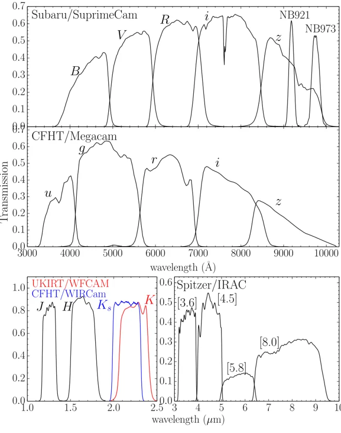
We used the SDF public data, which has limiting magnitudes of B = 28.45, V = 27.74, R = 27.80, i = 27.43, and z = 26.62 (2^′′ aperture, 3σ). We have also obtained new, deeper R-, i^′-, and z^′-band images. These images were constructed by stacking all the data taken from 2001 to 2008 in the course of a study of distant supernovae (Poznanski et al. 2007; Graur et al. 2011), containing almost 30 hours worth of integration time in total. The 3σ limiting magnitudes of these new deep images are 28.35, 27.72, and 27.09 at R-, i-, and z-bands, respectively. These are about 0.5 mag deeper than the SDF public data. The SDF was observed with several optical narrow-bands; two bands of these are used in this study. They are NB921 and NB973 centered at λc = 9196 and 9755 ˚A, respectively. All seven optical images, whose response curves are shown in Figure 1, were convolved to a common seeing size of 0.^′′98. The details of these image properties are summarized in Table 1.

In addition to the optical imaging, infrared imaging are conducted in the SDF. Near- infrared (NIR) images of J-, H-, K-band were taken with the WFCAM on the UKIRT (Casali et al. 2007) in March, April, and July 2010 (Hayashi et al., in prep). As shown in Figure 2, the SDF was covered by a mosaiced J-, H-, K-band image, although the depth was not uniform from field to field and the H-band images are not entirely covered the SDF. The seeing sizes of NIR images are 1.^′′1. Mid-infrared (MIR) images were obtained by the Infrared Array Camera (IRAC; Fazio et al. 2004) onboard Spitzer. IRAC uses four broad-band with central wavelengths at approximately 3.6, 4.5, 5.8, and 8.0µm. The details of these NIR and MIR image properties are summarized in Table 2 and 3, respectively, and the response curves are shown in Figure 1. While the FoV of the SDF would not be large enough to find a protocluster (actually the expected number density is ∼ 1 deg⁻², see Section 3.2 for detail), the SDF would, so far, be a better field to search for protoclusters at z ∼ 6 than any other fields due to the combination of deep and wide imaging. Therefore, only i-dropout galaxies will be investigated in the SDF. Although i-dropout galaxies are basically selected from two color diagram of i − z and z − J, i-dropout sample is selected by only i − z color in this thesis because the z-band image is much deeper than the J-band image. The J-band image will be secondarily used to reject apparent contaminations by M/L/T dwarfs.

2.1.2. CFHTLS Deep Fields

In addition to the SDF, we made use of publicly available data from the CFHTLS (T0007: Gwyn 2012), which was obtained by MegaCam mounted at the prime focus of the CFHT. The Deep Fields of the CFHTLS were used in this thesis, and it consists of four independent fields, each of which has about 1 deg² area (∼ 4 deg² area in total) with u-, g-, r-, i-, and z-bands. The CFHTLS Deep Fields provide two types of stacked images: one is generated using a sigma- clipped combination algorithm, and the other is using the standard median combination. Two sets of images of u-, g-, r-, i-, and z-bands are available for each type of stacked images: the

2. SAMPLE SELECTION 2.1. Photometric Data

85% and 25% best seeing images. We used the 85% best seeing images stacked by a sigma- clipped combination algorithm. The four independent fields have almost same depths within

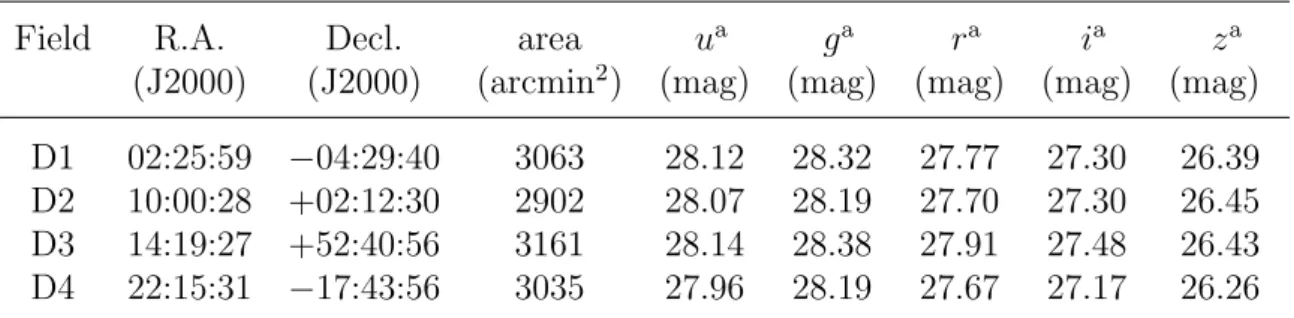
≲0.2 mag; therefore, the CFHTLS Deep Fields are one of the suitable fields to systematically study the large scale structure in high-redshift universe. The details, such as field centers, areas, and limiting magnitudes, of each field are summarized in Table 4. The seeing size and pixel scale of all images are ∼ 0.^′′7 and 0.^′′186, respectively.

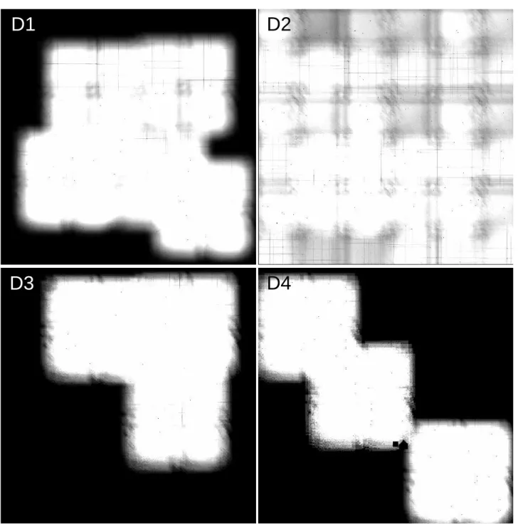
The CFHTLS Deep Fields are also observed in near-infrared wavelength of J-, H-, and Ks-bands by using WIRCam on CFHT, except the D2 Field’s J-band which was observed with WFCAM on UKIRT. We also used the public NIR data of the WIRCam Deep Survey (WIRDS T0002: Bielby et al. 2012). The FoV of WIRCam is 21^′ × 21^′, and the pixel scale is 0.^′′3/pixel. The publicly available images were rescaled to match the pixel scale of MegaCam and have the same image size with the optical images of CFHTLS Deep Fields in order to make it easy to run SExtractor (Bertin & Arnouts 1996) in double image mode. Only the part (∼ 50%) of each of the 1^◦ × 1^◦ CFHTLS Deep Fields was covered by NIR imaging; therefore, the pixel count out of the NIR FoV is set to zero in order to match the image size of CFHTLS Deep Fields. Five WIRCam pointings were taken in the D1 field, nine in D2, and three in D3 and D4 fields. The total area is ∼ 2.4 deg², and each field has almost uniform depth between pointings. The effective areas and the limiting magnitudes of WIRDS are summarized in Table 5. The field coverages of WIRDS are shown in Figure 3.

Table 1. Optical imaging data in the SDF

B V R i z NB921 NB973

3σ limiting magnitude^a(mag) 28.57 27.85 28.35 27.72 27.09 26.67 25.56

exposure time (hour) 10 6 27 28 31 15 15

aThe limiting magnitudes are measured with a aperture of 2 × FWHM.

Table 2. NIR imaging data in the SDF

filter pointing exposure time limiting mag.^a

(hour) (3σ)

detector 1 detector 2 detector 3 detector 4

J SDF1 2.5 23.86 23.88 23.97 23.76

SDF2 10 — 24.69 24.74 —

SDF3 9 24.74 — — —

SDF4 1.1 23.30 23.24 — —

H SDF1^b No data

SDF2 5 — 23.94 24.13 —

SDF3 5 24.23 — — —

SDF4^b No data

K SDF1 5 23.97 23.98 23.91 23.85

SDF2 5 — 24.13 24.12 —

SDF3 5 24.13 — — —

SDF4 0.4 22.75 22.59 — —

Note. — The subregions overlapped with the optical FoV are shown. The numbers of pointing and detector are the same as Figure 2.

aThe limiting magnitudes are measured with a aperture of 2 × FWHM. Since the sensitivities of the detectors are slightly different, the depth are dependent on both pointing and detector.

bThis subregion are not observed.

2. SAMPLE SELECTION 2.1. Photometric Data

Table 3. MIR imaging data in the SDF

3.6µm 4.5µm 5.8µm 8.0µm 3σ limiting magnitude^a(mag) 25.67 25.90 23.98 23.64

FWHM (arcsec) 2.2 2.1 2.3 2.3

aThe limiting magnitudes are measured with a aperture of 2 × FWHM.

Table 4. Optical imaging data in the CFHTLS Deep Fields

Field R.A. Decl. area u^a g^a r^a i^a z^a

(J2000) (J2000) (arcmin²) (mag) (mag) (mag) (mag) (mag) D1 02:25:59 −04:29:40 3063 28.12 28.32 27.77 27.30 26.39 D2 10:00:28 +02:12:30 2902 28.07 28.19 27.70 27.30 26.45 D3 14:19:27 +52:40:56 3161 28.14 28.38 27.91 27.48 26.43 D4 22:15:31 −17:43:56 3035 27.96 28.19 27.67 27.17 26.26

a3σ limiting magnitude in a 1.^′′4 aperture.

Table 5. NIR imaging data in the CFHTLS Deep Fields

Field area J^a H^a Ks^a

(arcmin²) (mag) (mag) (mag)

D1 1764 24.91 24.60 24.63

D2 2880 24.07 24.55 24.38

D3 1404 25.03 24.87 24.66

D4 1296 25.02 24.59 24.46

a3σ limiting magnitude in a 1.^′′4 aperture.

0.0

0.1

0.2

0.3

0.4

0.5

0.6

0.7 Subaru/SuprimeCam

B

V

R ⁱ

z

NB921

NB973

3000 4000 5000 6000 7000 8000 9000 10000

wavelength (˚ A)

0.0

0.1

0.2

0.3

0.4

0.5

0.6

0.7 CFHT/Megacam

u

g r _i

z

1.0 1.5 2.0 2.5

0.0

0.2

0.4

0.6

0.8

1.0 UKIRT/WFCAM

CFHT/WIRCam

J H ^K

^K

3 4 5 6 7 8 9 10

0.0

0.1

0.2

0.3

0.4

0.5

0.6 Spitzer/IRAC

[3.6] ^[4.5]

[5.8]

[8.0]

wavelength (µm)

T ra n sm is si on

Fig. 1.— The filter transmission curves.

2. SAMPLE SELECTION 2.1. Photometric Data

Fig. 2.— Arrangement of the individual WFCAM detectors in each pointing over the optical FoV of the SDF. Each square shows the FoV of the individual detectors, and the background image is the z^′-band image.

D1 D2

D3 D4

Fig. 3.— Weight maps of NIR imaging for the CFHTLS D1, D2, D3, and D4 fields.

2. SAMPLE SELECTION 2.2. Source Detection and Photometry

2.2. Source Detection and Photometry

Object detection and photometry in the optical and NIR images were performed by running SExtractor with double image mode on the images. In the SDF, we will focus on i-dropout galaxies because the depth of the z-band image is much deep as shown in Table 1; thus, we will use the z-band image as a detection image. On the other hand, in the CFHTLS Deep Fields, we made i-detected catalogs for u-, g-, and r-dropout galaxies as well as z-detected one for i-dropout galaxies. We can investigate large-scale galaxy distribution from z ∼ 3 even to z ∼ 6 by the combination of the deep images of the SDF and the wide images of the CFHTLS Deep Fields.

In the SDF, object detections were made in the z-band, corresponding to the rest-frame wavelength of 1200−1400 ˚A at z = 6. Then, the magnitudes, as well as photometric parameters, were measured in the other both bands at exactly the same positions and with the apertures of 2 × FWHM (2.0 arcsec) as in the detection-band image. We used the task “double image mode” of the SExtractor. Objects were detected when they have five connected pixels whose signal was higher than 2σ above the sky background RMS noise. Photometric measurements were made at the 2σ level. The objects are removed when they are in the masked regions with poor image quality. These regions are around bright stars, diffraction and bleed spikes from the bright stars. The regions near the frame edges were also masked where the depths were not uniform due to the dither pattern. The remaining effective area of analysis was 876 arcmin². Finally, ∼102,000 objects were detected down to z^′ = 27.09 (3σ limiting magnitude).

In the CFHTLS Deep Fields, the criteria of object detection were modified in order to optimize the image quality of CFHTLS Deep Fields obtained by MegaCam. We applied a Gaussian smoothing with FWHM = 3.0 pixels to the images in order to detect faint objects. After object detection, we used unfiltered images for photometry, and objects detected in low S/N regions were removed from the catalog. In MegaCam images, stars brighter than ∼ 9 mag produce a large halo, which has a radius of ∼ 3.5 arcmin. This resulted in larger mask areas compared with the SDF; the effective area of the CFHTLS Deep Fields is ∼ 83% of the FoV, but that of the SDF is ∼ 95%. Finally, ∼330,000–420,000 and 230,000–270,000 objects were listed in the i- and z-detected catalogues of CFHTLS Deep Fields down to the 3σ limiting magnitude of i- and z-bands in each field, respectively.

To estimate the detection completeness, we used the IRAF task mkobjects to create artificial objects on the original image. Artificial objects were created with the same PSF as real images, and were randomly distributed. To avoid blending artificial objects with real objects, we avoided positions close to the real objects with distances shorter than two times the FWHM of the real objects. We extracted the artificial objects using SExtractor with the same parameter set. In the z-band of the SDF, we generated 3000 artificial objects in the 23 to 29 magnitude range, and repeated this procedure 20 times. The detection completeness was more than 90% at z^′ = 25 and 70% at 3σ limiting magnitude. In the i- and z-bands of the CFHTLS Deep Fields, we generated 50,000 artificial objects in the 20–30 mag range, and extracted using SExtractor with the same parameter set. This procedure was repeated 10 times, and the detection completeness was evaluated as 70–50% at the 3σ limiting magnitude of i- and z-band in each field.

In the SDF, MIR images obtained by Spitzer/IRAC are also available. Photometry in MIR images should be performed more carefully than optical and NIR images, since PSFs in MIR

images are generally much larger than those in optical and NIR images. As a result, close objects tend to blend each other and the aperture flux of an object is likely to be contaminated by those of neighboring objects. To avoid the contamination, we conduct the following procedure to achieve an accurate photometry. First, we identified possible neighboring objects within a radius of 6.^′′0, which corresponds to 3 × FWHM of the IRAC images (Figure 4 (a)), around the targeted object in z-selected catalogue, and deblend them by using GALFIT (Peng et al. 2002). GALFIT is a software that fits 2D parametrized profile (e.g., S´ersic profile, Gaussian, and PSF) directly to the image, generating a model profile image (Figure 4 (b)) and a residual (raw − model) images. We use S´ersic profile for galaxies and PSF for stars on determining object profile in the z-band image. Then, GALFIT was rerun on each IRAC image, with the same profile parameters obtained in the z-band image. We assume that the profiles of z-band image are the same as those of the IRAC images. If close objects were too faint to fit, these objects are excluded from the fitting components in GALFIT. Finally, we obtained the residual images almost free from contamination from close objects (Figure 4 (c)). We conducted a photometry by using IRAF task phot with the aperture of 2 × FWHM to measure the MIR flux of targets. Note that it would be better to use the NIR images, especially K-band, which has closer wavelength coverage to the IRAC-bands, to determine a model profile instead of the z-band image. However, the depth of the NIR images of the SDF is much shallower (≳ 1.0 mag) than that of the MIR images, as shown in Table 2 and 3. Therefore, re-fitting in MIR images was sometimes failed based on the same profile parameters with the z-band image, especially using S´ersic profile, which has more fitting parameters (e.g., half-light radius, S´ersic index, and position angle) than PSF. In this case, we used PSF fitting instead of S´ersic profile fitting.

2. SAMPLE SELECTION 2.2. Source Detection and Photometry

Fig. 4.— The example of the removing contamination. (a) Raw images, (b) model images simulated by GALFIT, and (c) residual images in z^′, [3.6], [4.5], [5.8], and [8.0], respectively. The FoV of each panel is 12^′′× 12^′′.

2.3. Selection Criteria of Lyman Break Galaxies

We selected high-redshift galaxy samples by using Lyman break technique. This technique makes use of two color diagram to distinguish high-redshift galaxies from low-redshift galaxies and dwarf stars since high-redshift galaxies have unique spectral feature of Lyman break, which is caused by intergalactic medium (IGM) absorption. The selection criteria of u-, g-, r-, and i-dropout galaxies are followings (van der Burg et al. 2010):

u−dropout : 1.0 < (u − g) ∧ −1.0 < (g − r) < 1.2 ∧ 1.5(g − r) < (u − g) − 0.75,

g−dropout : 1.0 < (g − r) ∧ −1.0 < (r − i) < 1.0 ∧ 1.5(r − i) < (g − r) − 0.80 ∧ u > mlim,2σ, r−dropout : 1.2 < (r − i) ∧ −1.0 < (i − z) < 0.7 ∧ 1.5(i − z) < (r − i) − 1.00 ∧ u, g > mlim,2σ,

i−dropout : (i − z) > 1.5 ∧ u, g, r > mlim,2σ in the CFHTLS (B, V, R > mlim,2σ in the SDF), where mlim,2σ is a 2σ limiting magnitude. These selection criteria of u-, g-, and r-dropout galaxies are shown on two color diagrams of Figure 5. As shown in this figure, the possi- ble contamination of dropout selection, such as low-redshift elliptical galaxies having strong 4000˚A/Balmer break and dwarf stars, are effectively separated from high-redshift galaxies ac- cording to those criteria. Based on these criteria, for u-, g-, and r-dropout galaxies, we used i-band detected catalogues down to the 3σ limiting magnitude, and z-band detected one for i-dropout galaxies. The number and number counts of dropout galaxies in each field are shown in Tabel 6 and Figure 6, respectively.

We estimated redshift distribution of these dropout galaxies by using the population syn- thesis model code GALAXEV (Bruzual & Charlot 2003) and IGM absorption (Madau 1995). The estimate of IGM absorption relies on the distribution function of intergalactic absorbers of Lyα forest, Lyman-limit systems, and damped Lyα systems. It should be noted that, although we employed Madau’s model to estimate IGM attenuation in this thesis, some works proposed updated distribution functions based on recent observations (Meiksin 2006; Inoue et al. 2014). In GALAXEV, we simulated a large variety of galaxy spectral energy distributions (SEDs) using the Padova 1994 simple stellar population model. We assumed a Salpeter (1955) initial mass function (IMF) with lower and upper mass cutoffs mL = 0.1 M⊙ and mU = 100 M⊙, two metallicities (0.2 and 0.02Z⊙), and two types of star formation history of instantaneous burst and constant. We extracted model spectra with ages between ∼ 5 Myr and 500 Myr and applied the reddening law of Calzetti et al. (2000) with E(B − V ) between 0.0 and 1.0. The expected colors of high-redshift galaxies are estimated by convolving these simulated SEDs with filter transmission curves. The redshift distribution of u-, g-, r-, and i-dropout galaxies, applying our dropout selection criteria to these simulated galaxy catalogue are shown in Figure 7. The redshift evolution tracks of these simulated young star-forming galaxies are shown in Figure 5. We evaluated the contamination rate for these color-selection criteria. The sources of the majority of the contamination were dwarf stars and old elliptical galaxies, the latter being possible to satisfy the color criteria due to the 4000˚A/Balmer break. To estimate the contam- ination rate of dwarf stars, we use the TRILEGAL galactic model (Girardi et al. 2005). Since this model enables us to set up various structural parameters of thin disc, thick disc, halo, and bulge, we used exponential disk model with default values of scale length and height, and Cahbrier’s IMF was applied. The galactic latitudes were set to be the same as the observations (|b| = 82^◦ in the SDF, |b| ∼ 50^◦ in the CFHTLS Deep Fields). Then, photometry of simulated dwarf stars was calculated with CFHT/Megacam’s filter set. These simulated dwarf stars are

2. SAMPLE SELECTION 2.3. Selection Criteria of Lyman Break Galaxies

plotted in Figure 5 as green dots. Next, we simulated old galaxy SEDs using the GALAXEV, assuming two relatively high metallicities (Z⊙ and 2.5Z⊙), and extracted model spectra with age of 1 − 32 Gyr. The redshift evolution tracks of these simulated old galaxies are also plotted in Figure 5. As shown in this figure, the redshift tracks of old galaxies are away from all dropout selection regions. And, although a few dwarf stars are located only in the r- and i-dropout selection regions, the main locus of dwarf stars lie far from these regions. Actually, the con- tamination rate of dwarf stars in r-dropout samples is expected to be 2.2 − 7.8% depending on the galactic latitude of the CFHTLS Deep Fields (|b| = 40 − 60^◦), and the contamination rate in i-dropout samples is 3.4 − 6.4% in the CFHTLS Deep Field and 1.9% in the SDF, whose galactic latitude is +82^◦. Practical contamination rate would be slightly higher due to the photometric errors, as discussed later. Based on these simulation of dwarf stars and old galaxies, the dropout selection criteria used in this thesis are confirmed to be able to separate high-redshift galaxies from contaminations.

In addition to this estimate based on model predictions of dwarf stars and old galaxies, we checked the estimated contamination rate by comparing with observational works. According to the ERO catalogue by Miyazaki et al. (2003), few EROs can meet our dropout selection criteria, since the criterion of non-detection in shorter wavelength bands is effective to remove low- redshift galaxies. Actually, Malhotra et al. (2005) show that i-dropout objects with i − z > 1.3 do not include any EROs based on their spectroscopy. As for the contamination of dwarf stars, some dwarf stars can satisfy our dropout selection criteria based on the dwarf star catalogue by Hawley et al. (2002). Furthermore, from the combination of the star count model developed by Nakajima et al. (2000) and the luminosity function of dwarf stars from Gould et al. (1996); Zheng et al. (2001, 2004), the contamination rates are only about 1 − 6% at the galactic coordinates corresponding to our survey area. These contamination rates were found to be almost consistent with model predictions. Only for the SDF, J-band data is available in whole optical survey area though it is shallower than the optical images. According to Hawley et al. (2002), dwarf stars having i − z > 1.5 should have a very red color in NIR wavelength (z^′− J ≳ 2); therefore, typical dwarf stars can be detected even in the shallow J-band image. Therefore, we additionally imposed the criterion of z − J < 0.8 only on i-dropout objects detected in J-band. This would make contamination rate in i-dropout sample smaller. Based on these consideration, we assumed a contamination rate in our dropout selection of up to a few percent, mainly consisting of contamination from dwarf stars. In the subsequent analyses and discussions, we ignore the possible contamination by low-redshift galaxies.

Finally, we estimated the contamination rate resulted from photometric noise, which may scatter even lower-redshift sources to satisfy our dropout selection criteria, in addition to above intrinsic contaminations. We performed the following simple simulation, as same as in Wilkins et al. (2011a) and Bouwens et al. (2011b), to estimate the contamination rate due to the photometric noise. We first randomly choose brighter objects, and dim these bright source so as to match the magnitudes of our dropout samples by scaling the flux, then distribute these artificial objects on the original image using IRAF task mkobjects. We here assume faint objects have the same color distributions as that of bright objects whose photometric noise should be negligible. We extracted the artificial objects using SExtractor and impose our color criteria of dropout galaxies. The number of artificial objects in a given magnitude interval was chosen to be the same as the observed number of object in the same magnitude interval. We finally found

∼ 5 − 10% contamination rate in u-, g- and r-dropout samples and ∼ 15 − 20% in i-dropout

samples. Since the total number of i-dropout galaxies are much smaller (N_i ∼ 200) than those of u-, g-, and r-dropout galaxies (N ∼ 10³− 10⁴), even a few contaminations of photometric noise have a large effect on the contaminatin rate of i-dropout galaxies. It should be noted that these contaminants appeared almost randomly over the image in the repeated simulation, suggesting the contamination rate is homogeneous over the survey field and did not change the overdensity significance estimated in the next section.

Table 6. Number of dropout galaxies

Field area Nu Ng Nr Ni

(arcmin²)

D1 3063 17110 10416 2433 148 D2 2902 14515 11160 2539 231 D3 3161 21454 14896 2579 232 D4 3035 10484 11288 1926 188

SDF 876 – – – 258

2. SAMPLE SELECTION 2.3. Selection Criteria of Lyman Break Galaxies

−_{0.5 0.0 0.5 1.0 1.5}

g − r 0.0

0.5 1.0 1.5 2.0 2.5 3.0

u−g

u-dropout

−_{0.5 0.0 0.5 1.0 1.5}

r − i 0.0

0.5 1.0 1.5 2.0 2.5 3.0

g−r

g-dropout

−_{0.5 0.0 0.5 1.0 1.5}

i − z 0.0

0.5 1.0 1.5 2.0 2.5 3.0

r−i

r-dropout

20 21 22 23 24 25 26 27 28 z-band magnitude

0.0 0.5 1.0 1.5 2.0

i−z

i-dropout

Fig. 5.— Demonstration of dropout galaxy selection on two color and color-magnitude dia- grams. Thick black lines show the borders of dropout galaxy selection, and blue and cyan lines indicate redshift evolution tracks of young star-forming galaxies like LBGs (thin blue: age = 10 Myr and E(B − V) = 0.1, thick blue: age = 250 Myr and E(B − V) = 0.1, thin cyan: age = 10 Myr and E(B − V) = 0.4, and thick cyan: age = 250 Myr and E(B − V) = 0.4). Three red lines are redshift evolution tracks of elliptical galaxies at z ∼ 0-1.5 with ages of 1, 7, and 22Gyr, and green dots are dwarf stars estimated by the TRILEGAL galactic model (Girardi et al. 2005). Note that redshift evolution tracks in the i-dropout panel can shift horizontally depending assumption of stellar mass since the x-axis of the i-dropout panel is magnitude not color.

20 21 22 23 24 25 26 27 i-band magnitude (mag)

10⁻⁴ 10⁻³ 10⁻² 10⁻¹ 10⁰ 10¹

u-dropout

cumulativenumberdensity(arcmin−2 )

D1 D2 D3 D4

20 21 22 23 24 25 26 27

i-band magnitude (mag) 10⁻⁴

10⁻³ 10⁻² 10⁻¹ 10⁰ 10¹

g-dropout D1 D2 D3 D4

24 25 26 27

i-band magnitude (mag) 10⁻⁴

10⁻³ 10⁻² 10⁻¹

10⁰ _r-dropout D1 D2 D3 D4

25.0 25.5 26.0 26.5

z-band magnitude (mag) 10⁻⁴

10⁻³ 10⁻²

10⁻¹ i-dropout SDF D1 D2 D3 D4

Fig. 6.— Cumulative number counts of the u-, g-, r-, and i-dropout galaxies. The detection completeness was corrected. Although, in the SDF, i-dropout galaxies were selected down to the 3σ limiting magnitude of 27.09 mag, the drawing range of z-band is limited to 26.5 mag in order to make it clearer to check consistency between the SDF and the CFHTLS.

2. SAMPLE SELECTION 2.3. Selection Criteria of Lyman Break Galaxies

2.5 3.0 3.5 4.0 4.5 5.0 5.5 6.0 6.5 7.0

redshift

0.0

0.2

0.4

0.6

0.8

1.0

fr ac ti on

u-dropout g-dropout r-dropout i-dropout

Fig. 7.— Expected redshift distribution of u-, g-, r-, and i-dropout galaxies.

3. PROTOCLUSTER CANDIDATES

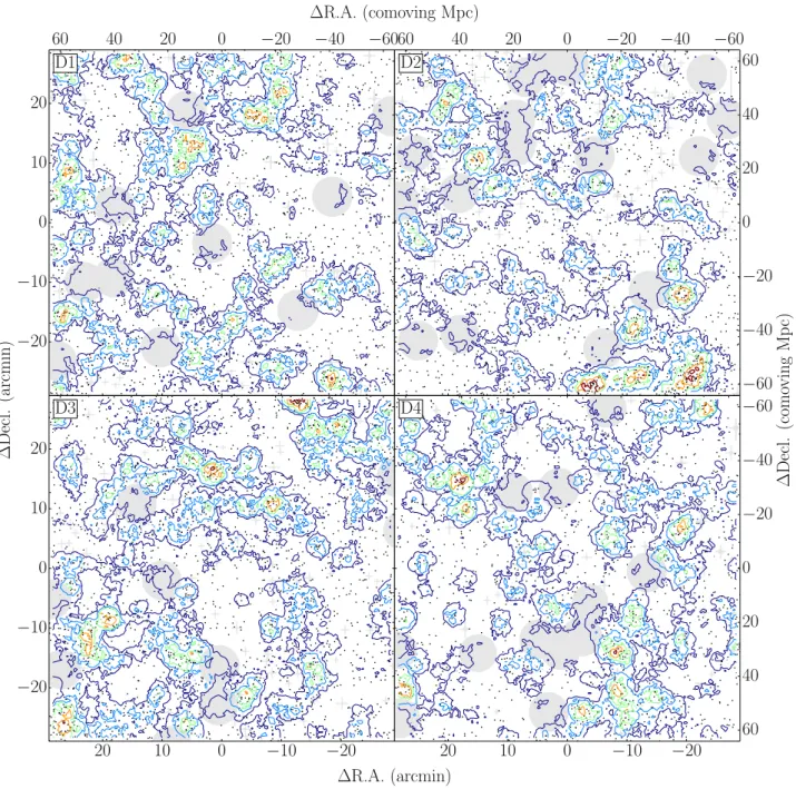
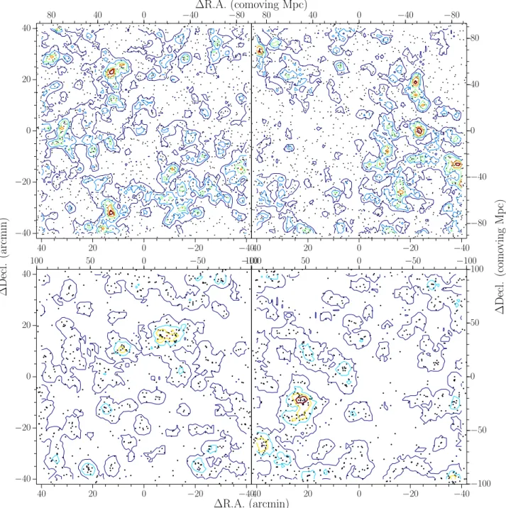
3.1. Sky Distribution and Overdensity

There are various methods to quantify galaxy distribution and clustering in the literature. Although spectroscopic observations would be the most direct and accurate methods to reveal three-dimensional structure of galaxies, they usually require a lot of telescope time. It is also suffers from incompleteness in a redshift space due to OH sky emissions and bias to easily identified emission line galaxies. To overcome these problems, many methods to use projected two-dimensional distributions of galaxies have been proposed. In the local universe, many effective methods are available based on rich data sets, such as tests of the asymmetry, the angular separation, and density contrasts of the structure (West et al. 1988), the adaptive- kernel based DEDICA algorithm (Pisani 1993, 1996; Ramella et al. 2007), the average two-point correlation function statistic (Salvador-Sole et al. 1993), and wavelet analysis (Flin & Krywult 2006). Using N -body simulation of dark matter, Arag´on-Calvo et al. (2007) have proposed the multiscale morphology filter to identify cosmic web and to extract galaxy distribution. While there are many sophisticated methods to quantify structures in the local universe, they are almost impossible to apply to the high-redshift universe where most of faint galaxies would be missed, and even if galaxies were detected down to faint end, its survey area is usually too small.

Simple methods to measure the local number density are commonly used to define environ- ments in the high-redshift universe: defined by the separation from N th nearest neighbour or the number of galaxies in a fixed aperture. Muldrew et al. (2012) have studied these two meth- ods’ advantage and disadvantage by using mock galaxy catalogue. Nearest neighbour method probes the internal properties of the halo, when neighbour number, N , is small enough. In con- trast, fixed aperture method can probe the halo as a whole: larger overdensity values indicate that massive halos are embedded. The comparison between nearest neighbour and fixed aper- ture methods were expanded to higher redshift by Shattow et al. (2013). They have found that nearest neighbour method tends to show larger scatter in the correlation between projected real (three-dimensional) overdensity. Fixed aperture method indicates better correlation between projected overdensities at z = 2 and real overdensity at z = 0.. From these considerations, fixed aperture method would be better to search protoclusters.

Based on the dropout samples described in Section 2.3, we have estimated the local surface number density by counting dropout galaxies within a fixed aperture in order to determine the overdensity significance quantitatively. A radius of a aperture has to be properly set according to the spatial scale of protoclusters. In the local universe, typical value of R200 for X-ray clusters is 0.5 Mpc. This indicates that, at least, > 0.5 Mpc radius is required to enclose most of protocluster members since it is expected that the distribution of protocluster members is wider than that of local clusters based on hierarchical structure formation model. On the other hand, Arag´on-Calvo et al. (2010) have predicted that galaxies are falling on clusters non-spherically through the filaments of cosmic web; thus, too large aperture will wash out the overdensity signal of protoclusters. Chiang et al. (2013) have estimated the typical radius of protoclusters at 2 ≲ z ≲ 5 by using the combination N -body simulation (Springel et al. 2005) and the semi-analytic galaxy formation model (Guo et al. 2011). Their defined radius corresponds to the size in which about 65% of the mass in bound halos and 40% of total