本文 Thesis 総合研究大学院大学学術情報リポジトリ A1901本文

(1)

The Galaxy–Halo Connection Across Cosmic History

Shogo Ishikawa

Department of Astronomical Science

School of Physical Sciences

SOKENDAI (The Graduate University for Advanced Studies)

(2)

ACKNOWLEDGMENTS

I am deeply grateful for my supervisor, Professor Nobunari Kashikawa, for his continuous supports of my research and the Ph.D. life in NAOJ. He devoted his precious time to discuss and improve my work, and gave me useful comments and inspirations whenever I got into difficulties. I have learnt a lot of things from him, and all of his teachings, remarks, and the attitude and the passion for research are my valuable assets in my life.

I would like to show my deep appreciation for Professor Tadayuki Kodama and Dr. Takashi Hamana, who are also my supervisors in SOKENDAI/NAOJ. They supported my research and gave useful comments from various aspects to improve my study and papers.

I am grateful for my colleagues and the collaborators of this research, Dr. Jun Toshikawa, Mr. Yoshifumi Ishizaki, Mr. Masafusa Onoue, Mr. Hisakazu Uchiyama, Dr. Masayuki Tanaka, Dr. Yuu Niino, and Dr. Kohei Ichikawa. I also thank people in Optical and Infrared Astronomy Division in NAOJ, people in Department of Astronomical Science in SOKENDAI, Subaru Telescope, and my friends.

Finally, I would like to show my deep and sincere gratitude to my parents, Noboru Ishikawa and Yuko Ishikawa, my sister, Mayu Moriyama (Ishikawa), and my grandparents, Tetsuzo Suzuki and Sumi Suzuki, for their understanding, helps, supports, and continuous encouragements to me.

(3)

ABSTRACT

In this thesis, I discuss the relationship between observable galaxies and their underlying invisible host dark haloes over the global cosmic time at z = 0 − 5 based upon the precision clustering analyses. At each redshift, I collect a large number of galaxy samples enough to obtain high-quality two-point auto angular correlation function (ACF), which is a useful estimator to measure the strength of galaxy clustering quantitatively. Furthermore, the high accurate ACFs enable to carry out more precise clustering analyses using a “halo occupation distribution (HOD)” formalism, which characterizes the occupation number and the distribution of galaxies within the virialized dark haloes as a function of the dark halo mass.

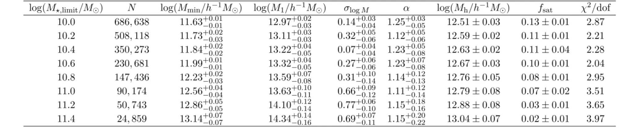
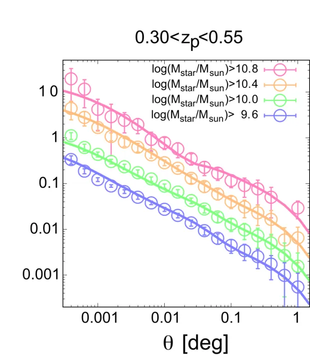
At low-redshift (z < 1.4) Universe, I collect numerous galaxy samples using the data of the Hyper Suprime-Cam Subaru Strategic Program (HSC SSP) Wide-layer. By using the photometric images with the extremely wide survey area taken by the Subaru/Hyper Suprime-Cam, I collect a large number of massive galaxies (M_⋆ > 10¹¹M_⊙) up to z = 1.4 as well as the less massive galaxies down to the limiting magnitude of i < 25.5 mag. Deep optical multi-wavelength images enable to apply a spectral energy distribution (SED) fitting technique to derive the stellar mass and the photometric redshift of each galaxy sample with high accuracies. I divide galaxy samples into subsamples according to their photometric redshift and the stellar mass in order to investigate the dependence of the clustering properties upon the physical properties by computing the ACFs of each subsample. Thanks to the numerous galaxy samples, derived ACFs show excellent S/N ratios, and the HOD model is able to reproduce the observed ACFs over all magnitude ranges. The mean halo masses of low-z dark haloes increase monotonically with increasing the stellar-mass limits and the cosmic time, indicating the evidence that massive haloes host massive galaxies and the halo growth via halo mergers. Our observed stellar-to-halo mass ratios (SHMRs) are in good agreement with the theoretical model of Behroozi et al. (2013b), although the slope at high-mass end shows a deviation from the model prediction.

The epoch at z ∼ 2, known as the “cosmic noon”, is important era to study formation and evolution of galaxy; however, it has been very difficult to construct a large number of galaxy samples, which is essential to carry out the precision clustering analyses. By combining our original data with publicly available data, I apply BzK/gzK selection to the wide-field imaging data over 5.2 deg², which is the largest-ever survey area of the BzK/gzK study. I select 41, 112 sgzK galaxies down to K_AB< 23.0. The ACFs based upon the largest sgzK sample with high quality enable to perform the HOD analysis. The mean halo mass and the HOD mass parameters are found to increase monotonically with increasing K-band magnitude, suggesting that more luminous sgzK galaxies reside in more massive dark haloes. Following the dark halo mass evolution using the extended Press–Schechter formalism and the number evolution of satellite galaxies in a dark halo, I find that faint Lyman break galaxies at z ∼ 4 could evolve into the faintest sgzK galaxies (22.0 ≤ K^AB ≤ 23.0) at z ∼ 2 and into the Milky-Way-like galaxies or elliptical galaxies in the local Universe, whereas the most luminous sgzK galaxies (18.0 ≤ KAB ≤ 21.0) could evolve into the most massive systems in the local Universe. In addition, the SHMRs of the sgzK galaxies are found to be consistent with the theoretical prediction, as well as the previous observational results at z ∼ 2.

At high-redshift (z > 3) Universe, I carry out the HOD analysis using the dropout galaxy samples at z ∼ 3, 4, and 5 using the Canada–France–Hawaii Telescope Legacy Survey (CFHTLS) Deep Field. Deep- and wide-field images of the CFHTLS Deep Survey enable to obtain sufficiently accurate ACFs to apply the HOD analysis. The mean dark halo masses, ⟨Mh⟩ = 10^11.7−12.8^h⁻¹^M⊙, is found to

(4)

increase with the stellar-mass limit. The threshold dark halo mass to possess a central galaxy within dark haloes, M_min, show almost identical behavior to their stellar mass, compared to low-z with the same stellar-mass limit, whereas the threshold dark halo mass to possess one satellite galaxy, M₁, show systematically higher values at z = 3 − 5 than those of low-z over the entire stellar-mass range. The satellite fractions, which represent the percentages of the satellite galaxy with respect to the total samples, are found to be significantly small compared to z ∼ 2, indicating the drastically increase of satellite galaxies from z = 3 − 2. Along with the high M1 values and the low satellite fractions of high-z galaxies, satellite galaxies form inefficiently within dark haloes at high-z. Assuming the main-sequence of star-forming galaxies, I computed the SHMRs, which is found to agree with those derived using the SED fitting method. The observed SHMRs are highly consistent with the theoretical predictions based on the abundance-matching method within 1σ confidence intervals. The pivot halo mass, M_h^pivot, which is the mass at the most efficient star-formation in galaxies, is, for the first time, found to increase with cosmic time at z > 3, and the SHMRs at M_h^pivotshow little evolution, indicating that mass growth rates of stellar components and dark haloes are comparable at 3 < z < 5.

From the precision clustering/HOD analyses, I firstly achieve to trace the redshift evolution of M_h^pivot across cosmic history by observations. The evolution of M_h^pivot is follows the theoretical prediction of Behroozi et al. (2013b): M_h^pivot increases with decreasing the redshift at z = 3 − 5 and has a peak at z ∼ 2, which is known as the highest star-formation era, and then decrease the star- formation efficiency with increasing the cosmic time at z = 2 − 0. This result of the redshift evolution of star-formation efficiencies is consistent with the theoretical models (e.g., Behroozi et al. 2013a,b; Moster et al. 2013) as well as the observational results (e.g., Hopkins & Beacom 2006). Moreover, I find that M_h^pivot to be almost unchanged around log(M_h^pivot/M_⊙) = 12.1 ± 0.2 over cosmic time at 0 < z < 5 and conclude that galaxy formation is ubiquitously most efficient near a halo mass of

⟨Mh⟩ ∼ 10¹²^M⊙ over cosmic time.

(5)

LIST OF ABBREVIATIONS

ABBREVIATION DESCRIPTION

ACF Two-Point Angular Auto Correlation Function BAO Baryon Acoustic Oscillation

CDM Cold Dark Matter

CFHTLS Canada–France–Hawaii Telescope Legacy Survey CLF Conditional Luminosity Function

HOD Halo Occupation Distribution

HSC Hyper Suprime-Cam

LBG Lyman break galaxy

NIR Near Infra-Red

SED Spectral Energy Distribution SHMR Stellar-to-Halo Mass Ratio

SMOKA Subaru–Mitaka–Okayama–Kiso Archive SPH Smoothed Particle Hydrodynamics

WIRDS WIRCam Deep Survey

(6)

1. INTRODUCTION

1.1. Dark Matter and Structure Formation

1.1.1. Large-scale structure of the Universe

After “the Great Debate” about the scale of the Universe between Harlow Shapley and Heber Curtis, spiral nebulae have been recognized as extragalactic objects like our Milky Way Galaxy. Before that, some studies have reported that gaseous emission lines of nebulae except for the Andromeda Nebula show red-shifted spectra (e.g., Slipher 1917), indicating that most of the extragalaxies go away from our galaxy. Georges Lemaˆıtre interpreted the redshift of extragalaxies is originated from the expansion of the Universe (Lemaˆıtre 1927) based upon the general relativity theory, which is constructed by Albert Einstein (Einstein 1911, 1916), and Edwin Hubble discovered a tight correlation between the recession velocities of galaxies (equivalent to galaxy redshifts) and their radial distances, which is known as “Hubble’s law” (Hubble 1929). Above the historical studies have established the picture of “Galaxy Universe”: the Universe is composed of numerous galaxies.

Using the redshift of galaxy as a quantity of galaxy distance, a distribution map of galaxies can be drawn. A first attempt to draw the 3D galaxy distribution map was the Center for Astrophysics (CfA) Redshift Survey, which carried out the spectroscopic galaxy observations to measure the redshifts of the large number of galaxy at Harvard-Smithsonian Center for Astrophysics (Huchra & Geller 1982; Huchra et al. 1983). The CfA survey, which is a pioneering redshift survey, gave great insights into knowledge of structure of the Universe and opened the door for the idea of the hierarchical structure model of the Universe in units of galaxies; however, the number of spectroscopically observed galaxy was about 2, 000 and the observable redshift was limited for the local Universe (z ∼ 0.05). By advancing the capabilities and efficiency of the observational instruments, many ambitious redshift surveys were implemented to achieve more precise descriptions of the galaxy 3D map by increasing the number of galaxy and limitation of redshift for the purpose of revealing the large-scale structure of the Universe.

The second CfA Redshift Survey (CfA2 Survey) started in 1984 and collected ∼ 20, 000 local bright galaxies in the northern sky. de Lapparent et al. (1986) firstly showed the map of galaxies by slicing the survey area of CfA2 Survey with narrow declination range (∆decl ∼ 6 degrees with ∆R.A.

∼ 135 degrees) and Geller & Huchra (1989) discovered a supercluster that consists of a lot of galaxy clusters (Figure 1). That amazingly vast galactic filament was termed “the Great Wall” (the scale of the Great Wall is estimated beyond 500 million light years) and it was also found that the Great Wall is surrounded by a wide area with extremely low galaxy density, known as a “cosmic void”.

The Sloan Digital Sky Survey (SDSS; York et al. 2000) is the largest redshift survey that is carried out both the multi-wavelength photometric observation as well as the spectroscopically observation using a wide-angle optical telescope mounted at Apache Point Observatory. This survey covered

∼ 12, 000 deg², which corresponds to ∼ 1/4 of the total sky, by five optical photometric images (u-, g-, r-, i-, and z-band; Fukugita et al. 1996) and selected about 375 million objects. The targets of the spectroscopic observation were selected based upon above the photometric observation and redshifts of about one million galaxies and 100, 000 quasars were confirmed. Gott et al. (2005) produced the map of the Universe from the scale of the Kuiper-Belt objects in our solar system to z ∼ 1.69 using the SDSS data and discovered an ”SDSS Great Wall” of galaxies with length of ∼ 1.37 billion light

(11)

1.1. Dark Matter and Structure Formation

Figure 1.— The galaxy distribution map drawn by the second CfA Redshift Survey (CfA2 Survey). In this figure, about 1, 100 spectroscopically observed galaxies are plotted. The filamentary structure of galaxies can be seen. It is noted that the long-drawn galaxy distribution around the center of the figure is not real structure but the effect of a Finger-of-God. This figure is originally presented in Geller & Huchra (1989) and credit of this figure is the Smithsonian Astrophysical Observatory.

years (∼ 423 Mpc), which is the largest structure in the Universe.

1.1.2. Dark side of the Universe

The 3D map of the Universe drawn by the extensive redshift surveys revealed there are a lot of structures such as filaments, voids, sheets, and nods, and the hierarchical structure of the present-day Universe (galaxies, galaxy groups, galaxy clusters, and galaxy superclusters) is formed by combined those structures complexly. However, it is known that the total amount of baryonic mass is quite small to form the large-scale structure of the Universe which can be seen in present-day Universe within Hubble time (which is an approximately age of the Universe calculated by an inverse Hubble constant, 1/H₀ ∼ 14.4 Gyr) by numerical simulations, known as the “missing mass problem”. To explain the shortage of the total amount of mass of the Universe and the anisotropy of the cosmic microwave background radiation (CMB), some cosmological models have been proposed to compensate the missing masses of the visible matters.

One of the most leading hypothesis to describe the picture of the Universe is a “ΛCDM” (e.g., Turner et al. 1984; Davis et al. 1985) paradigm, which is constructed based upon the idea of the “cold dark matter” model (CDM; Peebles 1982; Bond et al. 1982; Blumenthal et al. 1984). Dark matter is a hypothetical matter to fill a gap of the lack of the total mass of the Universe. The original idea of dark matter has been proposed by Fritz Zwicky to explain the mass gap between the galaxy cluster and field spiral galaxies (Zwicky 1933, 1937). He investigated the mass-to-luminosity ratio of the Coma galaxy

(12)

cluster and local Kapteyn stellar systems and reported that the mass-to-luminosity ratio of Coma cluster is M/L ∼ 500, whereas each Kapteyn system shows M/L ∼ 3, indicating that galaxy clusters are bounded by more massive gravitational system compared to field galaxies, and galaxy clusters are not the accumulated objects of galaxies. Another evidence for the existence of dark matter is a rotation curve of spiral galaxies. Rubin & Ford (1970) measured rotational velocities of the arms of Andromeda galaxy as a function of the radius from the galaxy center, and reported that radial velocities do not follow the Keplerian motion, showing the constant rotational velocity, irrespective of its radius. Many observational studies support the flat rotational velocity for spiral galaxies (e.g., Kent 1987; Sofue & Rubin 2001), and infer that invisible matter is extended to the outer regions of spiral galaxies to keep the rotational velocity constant. In addition, there are a lot of observational evidence for supporting the existence of dark matter such as the X-ray observation (e.g., Clowe et al. 2006; Akerib et al. 2014) and the weak gravitational lensing effect (e.g., Massey et al. 2007; Miyazaki et al. 2015).

Above problems (the missing mass problem and the rotation velocity problem) and observational results can be naturally explained by introducing the invisible matter in structure formation model. Some dark matter candidates have been proposed from the astrophysical aspect (massive astrophysical compact halo objects; MACHOs) and the aspect from the elementary particle theory (weakly inter- acting massive particles; WIMPs). MACHO is a baryonic candidate of dark matter that is too faint to detect by observations such as black holes, neutron stars, white and brown dwarfs, and planets. However, recent observations show that Big Bang nucleosynthesis model cannot produce the total amount of baryon enough for dark matter (Dar 1995) and the total mass of MACHO is much smaller than the expected mass of dark matter (Tisserand et al. 2007); thus, it is not expected that MACHO hardly contributes the total mass of dark matter. WIMPs is an elementary particle candidate of dark matter and it is assumed that they do not show the electromagnetic interaction, only show the gravitational interaction. Due to the achievement to approximately reproduce the large-scale structure of the Universe seen today by the cosmological simulations with WIMPs, it has been regarded that the possible candidate for dark matter is likely to be WIMPs, although it is still unclear which elementary particle is WIMPs.

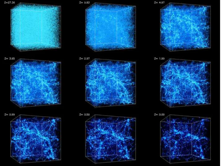
By introducing dark matter and investigating the evolution of the distribution across the cosmic time by the cosmological N -body simulations, it is found that dark matter gradually forms clumpy structures by congregating together by their gravity. Thanks to the high-quality capability of recent calculating equipments, one can trace the evolutionary history of dark matter distribution from z ∼ 130 to z = 0 and very small dark matter clumps by the latest cosmological dark matter N -body simulations, e.g., the Millennium simulation (Springel et al. 2005), the Bolshoi simulation (Klypin et al. 2011), and the MultiDark simulation (Prada et al. 2012), due to the high particle mass resolution as well as the spatial resolution. Figure 2 is an example of the cosmological N -body simulation with dark matter. One can find the clumpy and the filamentary structure in the simulation boxes, which are similar structure seen in the 3D map of the galaxies.

In summary, both the observational problems such as the missing mass problem and the constant rotation curve of the spiral galaxies as well as the theoretical problems to reproduce the large-scale structure of the Universe by the cosmological simulations are resolved simultaneously by introducing the assumed matter, termed dark matter. Considering the results of the cosmological simulations and the observational constraints, the candidate of dark matter is preferable to be massive elementary

(13)

1.1. Dark Matter and Structure Formation

Figure 2.— Redshift evolution of dark matter distribution from z = 30 (top left) to z = 0 (bottom right) by the cosmological N -body simulation. The box size is 43 Mpc. One can find the clumpy and the filamentary structure in the simulation boxes. Credit of this figure is Kavli Institute for Cosmological Physics (KICP) at the University of Chicago.

(14)

particles with no electromagnetic interactions (CDM).

1.2. Galaxy–Halo Connection

According to the paradigm of the ΛCDM, all of galaxies form and evolve within the clump of dark matter, termed a “dark halo”. Therefore, the structure formation in the Universe is largely governed by dark matter. Understanding of the formation scenario of the large-scale structure of the Universe boils down to the question of 1) how dark matter and dark haloes, which are harbors of galaxies, have been evolved, and 2) how galaxies have formed and evolved within dark haloes. The dark matter distribution is well studied by the cosmological N -body simulations precisely (see Section 1.1.2); however, the detailed scenario of galaxies is still an outstanding question. One can largely gain insights into the structure formation model if observed galaxies can be connected to the underlying dark matter (Figure 3). Nevertheless, it is quite difficult to link galaxies to their host dark haloes because dark matter cannot be observed directly by the telescope.

Figure 3.— The image of the distribution of dark matter and galaxies obtained by the numerical simulation. Left panel shows the results of the cosmological N -body simulation at z ∼ 2 and the central panel is a simplified view of the network of dark matter. The right panel displays the sites of highly star-forming regions shown in yellow. The credit of this figure is The Virgo Consortium/Alexandre Amblard/ESA. Refer to Amblard et al. (2011) for more details.

There are various technique for the connection between galaxies and their host dark haloes, i.e., a galaxy clustering technique (e.g., Totsuji & Kihara 1969; Peebles 1980; Eisenstein et al. 2005; Zehavi et al. 2011), an abundance-matching method (e.g., Col´ın et al. 1999; Kravtsov & Klypin 1999; Vale

& Ostriker 2004; Conroy et al. 2006), and a weak-lensing technique (e.g., Tyson et al. 1990; Kaiser 1998; Bacon et al. 2000; Wittman et al. 2000). However, the galaxy clustering is the almost only method to relate high-redshift observed galaxies to dark haloes. In this section, I will give a detailed prescription how observed galaxies can be linked to their host dark haloes along the description of the galaxy clustering.

(15)

1.2. Galaxy–Halo Connection

1.2.1. Galaxy clustering

One of the most critical methods to connect observed galaxies to the underlying invisible dark matter is to use the galaxy clustering. Galaxy clustering represents how galaxies bound together by their gravity. Galaxies within massive dark haloes show high amplitude of the galaxy clustering because massive dark haloes strongly correlate with each other, whereas galaxies within less massive dark haloes show the weak clustering amplitude. Thus, one can unveil the properties of invisible dark haloes by investigating the strength of amplitudes of the galaxy clustering.

The pioneering study of the galaxy clustering is Totsuji & Kihara (1969), who firstly applied a two-point angular correlation function (ACF) for galaxy samples obtained by Shane & Wirtanen (1967) to estimate the galaxy clustering statistically. The ACF, which is practically described ω(θ), represents how galaxies distribute over random/uniform distribution with a separation angle of θ. A probability to find both a galaxy at an element of solid angle δΩ₁ and another one at δΩ₂ with a separation angle of θ simultaneously, δP (θ), can be written using the ACF as follows:

δP (θ) = ¯N [1 + ω(θ)] δΩ₁δΩ₂, (1)

where ¯N is an averaged surface density of galaxy on the celestial sphere. By defining the two-point real-space auto correlation function as ξ(r), which represents the excess of galaxy distribution over the random distribution with distance r in real-space, δP can be easily extended into real-space as,

δP (r) = ¯n [1 + ξ(r)] δV1δV2, (2)

where ¯n is an averaged number density of galaxy and δV is a comoving volume element. The ACF is quite useful quantity to estimate the galaxy clustering strength statistically; however, the drawback of the ACF is that one have to collect the sufficient number of galaxy samples to obtain ACFs with high S/N ratio.

Many observational studies attempt to reveal the relationship between various galaxies and host haloes via the clustering analysis. Zehavi et al. (2005, 2011) carried out precise clustering analyses using the large number of local galaxies obtained by the SDSS survey and discussed the correlation between galaxy properties and strengths of the galaxy clustering. Using the selection methods for the specific galaxy populations or the photometric redshift via the SED fitting technique (see Section 3.1.2), galaxy clustering analyses have been applied for galaxies at z > 1 (e.g., Adelberger et al. 2005; Kashikawa et al. 2006; McCracken et al. 2010; Wake et al. 2011; Coupon et al. 2012; Ishikawa et al. 2015). Furthermore, Barone-Nugent et al. (2014) computed the ACF at z ∼ 7.2 and derived the bias parameter (refer to Section 2.1.4) using the data of the Hubble eXtreme Deep Field (XDF; Illingworth et al. 2013) and the Cosmic Assembly Near-infrared Deep Extragalactic Legacy Survey (CANDELS; Grogin et al. 2011; Koekemoer et al. 2011).

By dividing galaxy samples into subsamples according to their baryonic properties such as stellar masses, luminosities, and magnitudes, one can discuss the dependence of the clustering properties on baryonic properties of galaxies. One can also reveal the relationship between the dark halo masses and the properties of galaxies; however, it is necessary to assume some analytical formulae and the approximated picture of a one-to-one correspondence between galaxies and dark haloes. Thus, more precise model is required to interpret observed galaxy clustering in terms of the realistic physical processes.

(16)

1.2.2. Halo occupation distribution model

A “halo occupation distribution” (HOD, e.g., Ma & Fry 2000; Seljak 2000; Berlind & Weinberg 2002; Berlind et al. 2003; van den Bosch et al. 2003a) is a powerful theoretical approach that relates the galaxy distribution to the dark matter distribution. The HOD formalism describes the galaxy distribution within the host dark halo by characterizing them from the perspective of the probability distribution P (N |M) that a halo of virial mass M contains N galaxies with specific physical properties, such as color or galaxy type. One of the advantages of the HOD formalism is that the HOD parameters have explicit physical meanings; this enables us to easily interpret the relationship between the galaxies and the host haloes.

The largest difference between the HOD framework and other galaxy–halo correspondence methods, such as the abundance-matching method, is that the HOD model is based on a more realistic halo model and does not assume a one-to-one correspondence between galaxies and host haloes. It is known that different types of galaxy pairs contribute to the ACF between large-angular scales and small-angular scales. At the small-angular scale, galaxy clustering is contributed to mainly by galaxy pairs that are located in the same dark halo, referred to as the “1-halo term”, whereas galaxy clustering at the large-angular scale is attributed to galaxy pairs that reside in different dark haloes, referred to as the “2-halo term”. These two components result in different power-law slopes of the ACF at the two angular scales; these characteristics are well described using the HOD formalism. In Figure 4, I present the conceptual diagram to represent what type of the galaxy pair is dominant for the HOD formalism at each angular scale.

The HOD model predicts a power spectrum of galaxies by assuming some analytical formulae for characterizing the dark haloes and the occupation manner of galaxies within dark haloes. The occupation of galaxies can be described by formulating the number of galaxies within dark haloes, N_tot(M_h), as a function of dark halo mass M_h. Total number of galaxies is composed of two types of galaxies: a central galaxy and satellite galaxies. One can describe the number of galaxies within dark haloes by considering the above galaxy types as N_tot(M_h) = N_cen(M_h) + N_sat(M_h), where N_cen(M_h) and N_sat(M_h) represent the number of the central and the satellite galaxies within dark haloes as a function of halo mass M_h. It is noted that N_cen(M_h) satisfies the condition of N_cen(M_h) ∈ [0, 1] because dark haloes cannot possess multiple central galaxies due to the definition of the central galaxy. Once the galaxy power spectrum from the HOD model is computed, one can derive a correlation function of galaxies in real space by the Fourier transformation using a so-called “Wiener-Khintchine relation”. The ACF can be derived by projecting the real-space two-point correlation function using a “Limber’s approximation” (Limber 1953). I plotted the galaxy power spectrum, real-space correlation function, and the projected ACF calculated by the HOD formalism in Figure 5. Detailed descriptions of the theoretical framework of the HOD formalism are given in Section 2.3.

1.2.3. Interpretation of observed galaxy clustering using the HOD model Recently, many studies use the HOD model to interpret the observed galaxy clustering signals in high-redshift Universe as well as local/low-redshift Universe. Zehavi et al. (2005) carried out the HOD analysis to investigate the dependence of the galaxy properties such as galaxy color or its luminosity on the galaxy clustering using the numerous local galaxy samples (200, 000 galaxies over 2, 500 deg²

(17)

Figure 4.— A conceptual diagram to explain the HOD formalism. Left figure is an illustration to represent how galaxies correlate with each other and right figure is the observed ACF and the best-fit HOD fitting. In the HOD model, massive dark haloes can possess one central galaxy and multiple satellite galaxies within them, whereas less massive dark haloes contain only one or no central galaxy. Within massive dark haloes, strong clustering of the central–satellite galaxy clustering and the satellite–satellite galaxy clustering can be observed (red arrows in left figure); these clustering signals appear at small-angular scales in ACFs, termed the “1-halo term” (dotted red line in right figure). On the other hand, at large-angular scale, only the galaxy clustering between central galaxies within different dark haloes (green arrows in left figure) appears to the ACF, termed the “2-halo term” (dotted green line in right figure). The observed ACF can be represented by the sum of each component (solid blue line in right figure), the 1-halo term and the 2-halo term. It is noted that the observed ACF of right figure is measured by the galaxies obtained by the HSC SSP survey at 0.80 < z_phot< 1.10 with stellar-mass limit of log (M_⋆/M_⊙) > 9.8.

(18)

0.01 0.1 1 10 100 1000 10000

0.1 1 1 0

P(k) [(h Mp c-1)3]

k [h Mpc-1]

0.1 1 10 100 1000 10000 100000

0.01 0.1 1 10

ξ(r)

r [h-1 Mpc]

0.001 0.01 0.1 1 10

0.001 0.01 0.1 1

ω (θ

)

θ [deg]

Figure 5.— The galaxy power spectrum, P (k), (left panel), the real-space two-point correlation function, ξ(r), (middle panel), and the ACF, ω(θ), (right panel) predicted by the HOD formalism. First, the HOD model compute the power spectrum of galaxies from the assumption of some analytical formulae and the galaxy occupation within dark haloes. Power spectrum can be transformed from Fourier space into real space using the Wiener-Khintchine relation, and the transformed function os the real-space two-point correlation function. The ACF is derived by projecting the real-space two- point correlation function using the Limber’s approximation. One can compare observed galaxy ACFs with the ACF calculated by the HOD model and investigate the properties of host dark haloes of galaxy samples by constraining the occupation of galaxies within dark haloes. The power spectrum, the real-space two-point correlation function, and the ACF presented in this figure are derived from the best-fit HOD model for galaxies obtained by the HSC SSP survey at 0.80 < z_phot < 1.10 with stellar-mass limit of log (M_⋆/M_⊙) > 9.8.

(19)

at z < 0.22) obtained by the second data release of SDSS survey, and Zehavi et al. (2011) extended their analyses by increasing the redshift range and the number of galaxy samples (700, 000 galaxies over 8, 000 deg² at z < 0.25) using the completed data of SDSS redshift survey (see Section 3.1.1).

As is the case with the local Universe, low-z Universe has been well investigated the relation between galaxies and their host haloes because of the easiness in collecting a large number of galaxy samples (e.g., Matsuoka et al. 2011; Wake et al. 2011; Coupon et al. 2012; Skibba et al. 2014; Coupon et al. 2015; Rodr´ıguez-Torres et al. 2016); however, z ∼ 2 Universe has not been well studies due to the difficulty of the sample selection. McCracken et al. (2010) collected the star-forming galaxies (sBzK galaxies) and passively evolving galaxies (pBzK galaxies) at z ∼ 2 using the “BzK selection technique” (Daddi et al. 2004) in the COSMOS field, and B´ethermin et al. (2014) firstly applied the HOD analysis on the sBzK galaxies using the photometric catalogue of McCracken et al. (2010). Moreover, Ishikawa et al. (2016) carried out precise clustering analysis and HOD analysis on star-forming galaxies at z ∼ 2, which is approximately twice sample number compared to McCracken et al. (2010) selected by Ishikawa et al. (2015).

It has been investigated in higher-redshift Universe (z > 3) compared to z ∼ 2 because the selection method of the high-redshift galaxy has already been established in the mid-1990s (e.g., Steidel et al. 1996) and they can be selected only using the optical images. Harikane et al. (2016) carried out clustering and HOD analyses of Lyman break galaxies at z = 4 − 7 by combining data of Hyper Suprime-Cam and publicly available data of Hubble Space Telescope. They investigated the redshift evolution of SHMRs but the accuracy of the clustering analysis is not good due to the small number of galaxy samples. Ishikawa et al. (2017) collected a large number of LBG samples enough to carry out precise clustering analysis in high-z Universe and confirmed the validity of the model prediction of the stellar-to-halo mass ratio presented by Behroozi et al. (2013b).

1.2.4. Beyond the “classical” HOD model

The HOD formalism has been developed to interpret galaxy clustering with relating the underlying dark matter and succeeded to reveal the relation between galaxies and host haloes; however, there is still room for improvement. For example, the HOD model does not assume that central galaxy should be brighter or heavier than satellite galaxies within the same dark haloes. Moreover, there is no condition that massive haloes should possess brighter or heavier galaxies compared to less massive haloes, provided that galaxies satisfy the threshold of the stellar mass (or the flux) for its sample selection. However, it seems oddly by considering the observational results; the central galaxy of galaxy clusters is the brightest galaxies among the member galaxy, termed a “brightest cluster galaxy (BCG)”, and the stellar masses of central galaxies monotonically increase with increasing their host haloes according to stellar mass–halo mass relations in the local Universe (e.g., Leauthaud et al. 2012; Kravtsov et al. 2014; Coupon et al. 2015).

To fill a gap between the “classical” HOD formalism as a toy model and realistic physical conditions, some improved HOD models have been proposed. The early attempt was to consider the constraint of the observed luminosity functions or the stellar-mass functions in the HOD model, known as a “conditional luminosity function model” (CLF; Yang et al. 2003; van den Bosch et al. 2003a) and a

“conditional mass function model” (CMF; Moster et al. 2010). The CLF model considers the average number of galaxies within the dark haloes with mass M_h_{, Φ(L|M}_h), with luminosities within the range

(20)

of L ± L/2, whereas the CMF model considers the average number of galaxies within the dark haloes with mass M_h, Φ(M_⋆_|M_h), with stellar masses within the range of M_⋆_{± M}_⋆/2. Therefore, one can say that the CFL and the CMF model is the differential form of the classical HOD model with respect to the luminosity or the stellar mass. By constraining the number of galaxies according to the luminosity or the stellar mass of galaxies, it seems to be resolved the issue that HOD model distributes galaxies regardless their baryonic properties. Nevertheless, both the luminosity functions and the stellar-mass functions are suffered from relatively large scatters and not observed correctly especially in high-z Universe. Leauthaud et al. (2012) carried out the HOD analysis for the galaxy samples at z ≲ 1 in the COSMOS field using an extended HOD model that is introduced the constrain of the parame- terized form of the stellar-to-halo mass ratio (Behroozi et al. 2010) constructed by Leauthaud et al. (2011). Moreover, Zu & Mandelbaum (2015) proposed another post HOD model to compensate the stellar-mass incompleteness of galaxy samples by introducing the observed stellar-mass function in the formulated HOD model, named an “iHOD model”, where i denotes “incompleteness”.

The classical HOD model assumes that galaxy clustering is primarily governed only by the halo mass, albeit other physical properties of dark haloes. However, recent studies have reported that galaxy clustering strengths also depend on the age of host haloes, known as a “halo assembly bias” (e.g., Gao & White 2007; Reed et al. 2007; Miyatake et al. 2016). Hearin et al. (2016) developed an improved HOD formalism, called a “decorated HOD model”, which is taken into account the effect of the halo assembly bias in their HOD model. Zentner et al. (2016) reanalyzed the galaxy clustering of the SDSS galaxies, which are originally analyzed by Zehavi et al. (2011), using the decorated HOD model and concluded that the halo assembly bias cannot be ruled out its possibility for the SDSS galaxies. Another big feature of the decorated HOD model is that this model uses the results of the cosmological N -body simulations for information of dark haloes instead of employing the analytical formulae of dark haloes; one assigns observed galaxies to dark haloes following the occupation manner of the HOD formalism in the similar manner as the abundance-matching method and the ACF from the decorated HOD model can be calculated by measuring the clustering of galaxies within the simulation box. However, we should keep in mind that detailed properties of the halo assembly bias is under discussion. Miyatake et al. (2016) found a strong correlation between concentrations of cluster member galaxies and the density fluctuations of dark matter using the local SDSS clusters; however, it is still unclear whether the above correlation can be applied for galaxy-size haloes and the more distant clusters. Tinker et al. (2016) investigate the correlation between halo ages and galaxy ages to identify the halo assembly bias using a galaxy group catalogue (Blanton et al. 2005) and concluded that massive galaxies show correlation between a large-scale environment and a large-scale density fluctuation, whereas the correlation between them cannot be seen for less massive galaxies (M_⋆ ≲ 10¹²M_⊙). Further elucidation of the halo assembly bias and improvement of the HOD model with the assembly bias may require future observations.

1.2.5. Stellar-to-halo mass ratio

Another method that can be used to relate the dark halo to the distribution of baryons in the dark halo is termed the “stellar-to-halo mass ratio” (SHMR), which is defined as the ratio between the dark halo mass and the galaxy stellar mass, represents the conversion efficiency from baryonic matter into stellar components within dark haloes. The SHMR has been the subject of many theoretical studies aiming to reveal or constrain the properties of galaxies and the conversion efficiency from

(21)

baryons into galaxies in dark haloes (e.g., Behroozi et al. 2010; Moster et al. 2010; Yang et al. 2012; Behroozi et al. 2013a,b). On the M_h versus M_⋆/M_h diagram, the SHMR has a peak at M_h _{∼ 10}¹²M_⊙, which corresponds to the most efficient mass, termed a “pivot halo mass” (M_h^pivot; Leauthaud et al. 2012), to convert from baryonic matter into stars, which is consistent with theoretical prediction (e.g., Blumenthal et al. 1984). However, the SHMR at the M_h^pivot is much smaller than the universal baryon fraction (Ωb/Ωm∼ 0.167) (e.g., Behroozi et al. 2010; Leauthaud et al. 2012; Yang et al. 2012), indicating that a part of baryon in dark haloes are not converted into stars. This characteristic dark halo mass is determined by the equilibrium of the suppression mechanism that star formation becomes equal between the shallow gravitational potential wells for less-massive dark haloes and active galactic nuclei (AGN) feedback, and high virial temperature of massive dark halo.

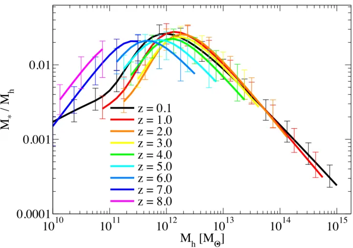
Yang et al. (2012) presented a functional form of the SHMR up to z ∼ 4 using the observational stellar-mass functions and the two-point correlation functions via the CLF model. Moster et al. (2013) carried out numerical simulations to constrain the SHMR at 0 < z < 4 with observational constrains of stellar-mass functions. They found that the most efficient halo mass shows mild redshift evolution; log (M_h^pivot/M_⊙) ∼ 11.8 at z = 0 and log (M_h^pivot^/M⊙) ∼ 12.5 at z ∼ 4, indicating that star formation in high-redshift preliminary takes place only in massive dark haloes. Behroozi et al. (2013b) predicted that the redshift evolution of the SHRM from z = 8 to z = 0 using numerical simulations. Figure 6 is the results of their SHMRs obtained by the numerical simulation with observational constrains of stellar-mass functions, specific star-formation rates, and cosmic star-formation rates at each redshift. They concluded that star formation is the most efficient at M_h _{∼ 10}¹²M_⊙ and its evolution is quite small at 0 < z < 5; however, there was a trend that the pivot halo mass became larger with increasing redshift from z = 0 to z = 3, and the conversion efficiency for the massive dark halo was the highest when 2 < z < 3. Besides above theoretical approach to the SHMRs, many studies tackle to reveal the details and the redshift evolution of SHMRs using the semi-analytical model (e.g., De Lucia & Blaizot 2007; Guo et al. 2011; Birrer et al. 2014; Somerville et al. 2015).

In addition to the theoretical works, observational studies have been revealed the SHMR, almost of which are implemented by clustering analyses. Leauthaud et al. (2012) carried out HOD analyses for z < 1 galaxies in the COSMOS field; they employed an improved HOD model that included the constraints of the SHMR of central/satellite galaxies, enabling them to investigate the SHMR of central and satellite galaxies separately. Leauthaud et al. (2012) showed that the M_h^pivot mass varies with the redshift, which is evidence of mass downsizing at 0 < z < 1, and the SHMR of satellite galaxies becomes dominant for massive dark halo (M_h > 10¹³M_⊙; Figure 7). Coupon et al. (2015) also investigated the SHMRs of galaxies at z ∼ 0.8 by adopting the HOD+SHMR model of Leauthaud et al. (2012) in the CFHTLenS (Heymans et al. 2012) and the VIPERS fields (Guzzo et al. 2014; Garilli et al. 2014). They showed an excess of the SHMR for massive dark haloes compared to the results of Behroozi et al. (2013b), indicating that the total amount of stellar components within massive haloes is dominant from the satellite galaxies.

Recent observational studies also reveal the SHMRs even at z > 1 Universe by overcoming the difficulties to estimate galaxy stellar masses as well as dark halo masses. McCracken et al. (2015) obtained galaxies at 0 < z < 3 by the SED fitting technique in the UltraVISTA field (McCracken et al. 2012). They calculated the SHMR up to z < 2.5; however, SHMRs at z > 1 are not estimated correctly due to the large scatters of the photometric redshifts. Ishikawa et al. (2016) carried out the HOD analysis on star-forming galaxies at z ∼ 2 and revealed the SHMR, showing that the decreasing

(22)

10

¹⁰

10

¹¹

10

¹²

10

¹³

10

¹⁴

10

¹⁵

M

h

^[M

O^●

^]

0.0001

0.001

0.01 M

*

/ M

h

z = 0.1

z = 1.0

z = 2.0

z = 3.0

z = 4.0

z = 5.0

z = 6.0

z = 7.0

z = 8.0

Figure 6.— The redshift evolution of the SHMRs calculated by numerical simulations (Behroozi et al. 2013b). In this simulation, they only considered the contribution of central galaxies; thus, these SHMRs are the relation of the central galaxies. The SHMRs are calculated using observational constraints of galaxy stellar-mass functions, specific star-formation rates, and cosmic star-formation rates from z = 0 to z = 8 at each redshift. This figure shows that the most efficient halo mass (M_h^pivot) is M_h^pivot_{∼ 10}¹²M_⊙ regardless its redshift and the values of the SHMRs at M_h^pivotdo not significantly change at z = 0 − 8. This figure is originally presented by Behroozi et al. (2013b).

(23)

10

¹¹

10

¹²

10

¹³

10

¹⁴

Halo Mass M

_200b

[ M ]

0.01

0.10 tot a l(M

*

)/ M

200b

WMAP5 _b/ _m

Sa^te lli^te

s Cent

rals

z = 0.37

Ω Ω

○・

Figure 7.— The results of the SHMRs of galaxies at z ∼ 0.37 in the COSMOS field derived by Leauthaud et al. (2012). They used the improved HOD model including the constrains of the SHMR, and investigate the relationship between galaxies and dark haloes by a joint analysis of the spatial galaxy clustering, the galaxy–galaxy lensing, and the stellar-mass function developed by Leauthaud et al. (2011). The total SHMR is attributed by central galaxies for less massive dark haloes and consistent with the results of Behroozi et al. (2013b), whereas satellite galaxies are dominant for massive dark haloes (M_h≳10¹³M_⊙). This figure is originally presented by Leauthaud et al. (2012).

(24)

trend of the SHMR of massive galaxies can be seen even at high-z. Harikane et al. (2016) calculated the SHMRs of quite less massive (M_⋆ _{∼ 10}⁷⁻⁹M_⊙) Lyman break galaxies (LBGs) at z = 4 − 7 using the archive data of the Hubble Space Telescope and the Subaru Telescope/Hyper Suprime-Cam. They found that the redshift evolution of their SHMRs was consistent with the theoretical predictions via the abundance-matching technique (Behroozi et al. 2013b), and baryon conversion efficiency at z ∼ 4 increased monotonically up to ⟨M^h⟩ ∼ 10¹²^M⊙. Moreover, Ishikawa et al. (2017) carried out HOD analyses on LBGs at z ∼ 3, 4, and 5 using the publicly available data of the Canada–France–Hawaii Telescope Legacy Survey (CFHTLS; Gwyn 2012) Deep Fields and achieved to calculate the M_h^pivot at z > 1 firstly. They showed increasing trend of M_h^pivot with increasing cosmic time at z > 3, and the SHMRs at M_h^pivot show little evolution, indicating that mass growth rates of stellar components and dark haloes are comparable at 3 < z < 5.

1.3. This Thesis

The ultimate goal of this study is to reveal how the large-scale structure of the Universe formed and evolved. To resolve this issue, it is necessary to unveil how galaxies formed and evolved within underlying dark haloes. Since the evolutionary history of dark matter, which are bearers of the structure formation, is well studied by the cosmological N -body simulation, one can gain insights into the structure formation scenario by linking galaxy evolution to the dark halo evolution. However, understanding of the scenario of galaxy formation and evolution is essential to complex physical mechanisms with baryons and it is difficult to research the evolutionary relationship among galaxy populations by tracing the evolution of their baryon characteristics.

Another approach to study the evolutionary history of galaxies is to trace the evolution of host halo masses of various galaxy populations. One can estimate the evolutionary model of galaxy to determine the properties of galaxies, including the dark halo mass, the stellar mass, the star-formation rate, and the morphology over cosmic time, and to compare these quantities with theoretical models. The dark halo mass of galaxies is a particularly important parameter to trace the mass assembly history of galaxies because, according to the ΛCDM model, dark haloes grow monotonically with cosmic time by merging, irrespective of the baryonic processes. However, the measurement of the mass of the dark halo is no straightforward. One of the most effective methods to determine the mass of dark haloes is to use the galaxy clustering.

Dark halo masses tell us the evolutionary connection among galaxy populations; however, this method just gives a possibility for the galaxy evolution since baryonic evolutions are not considered. Therefore, other properties of galaxies should be taken into account to establish the valid evolutionary history of galaxies. It is difficult to obtain baryonic properties of galaxy, such as the stellar mass, age, star-formation rate, and the amount of dust extinction; however, one can derive those quantities by carrying out the SED fitting technique, provided that multiple color photometric data are available. In addition, one can derive the distribution pattern of galaxies by applying the HOD formalism. The evolutionary history can be constructed validly by investigating the evolution of satellite fractions and SHMRs, as well as the evolution of dark halo masses among various galaxy populations at various redshifts.

In this thesis, I discuss the relationship between galaxies and their host dark haloes at z = 0.3−5.4

(25)

1.3. This Thesis

based upon the results of precision clustering analyses. Thanks to quite wide survey areas, I succeed to collect the large number of galaxy samples enough to obtain the high-quality ACF at each redshift. Furthermore, our high accurate ACFs enable us to carry out more precise clustering analyses using the HOD formalism. In addition, I reveal the baryonic properties of galaxies using multi-wavelength data, especially photometric redshifts and galaxy stellar masses, by applying the SED fitting technique and investigate the properties of dark haloes by the properties of baryons. By combining both aspects of galaxies of baryons and dark haloes, I target to unveil the evolutionary history of galaxies from z ∼ 5.4 to z = 0.3 by tracing the evolution of baryonic properties such as satellite fractions and SHMRs, as well as the evolution of host dark halo masses.

This thesis is organized as follows. In Section 2, I present a theoretical framework of the galaxy clustering and the HOD formalism. The results of clustering and HOD analyses are given in Sec- tion 3, 4, and 5: in Section 3, I show the results of clustering using/HOD analyses at 0.3 < z < 1.4 using the data of the Hyper Suprime-Cam Subaru Strategic Project (HSC SSP) survey, the relations between star-forming galaxies at 1.4 < z < 2.5 (sgzK galaxies) and their host haloes by accurate clustering analyses based on the wide-field survey is presented in Section 4, and the results of the precision clustering/HOD analyses and the details and the evolution of SHMRs of LBGs at 2.5 < z < 5.4 is given in Section 5. In Section 6, I give the organized discussion across cosmic history using the above results. Conclusion of this thesis and future prospects are presented in Section 7. Adopted cosmological parameters and the typical physical scales under those parameters are shown in the overview of each section.

(26)

2. A THEORETICAL FRAMEWORK OF GALAXY

CLUSTERING ANALYSIS

2.1. Galaxy Clustering Statistics

2.1.1. Two-point angular auto correlation function

A Two-point angular auto correlation function (ACF) is an extensively used physical quantity to estimate the strength of the galaxy clustering statistically. The first attempt to apply the correlation function to measure the strength of galaxy clustering is Totsuji & Kihara (1969), and ACFs are widely accepted as a useful tool for clustering analysis after introduction of the famous textbook (Peebles 1980).

The very early studies of galaxy clustering (e.g., Davis et al. 1978; Phillipps et al. 1978) simply count the separation angles of galaxies because the number of galaxies that are confirmed their redshifts are quite small. Those early studies revealed that the ACF follows the power law as

ω(θ) = Aωθ^1−γ, (3)

where A_ω is an amplitude of the ACF and γ is a power-law slope. The simple counting method is, however, no longer used for almost all today’s clustering analyses, including my study of this thesis, because of dealing enormous galaxy samples. Therefore, various ACF estimators have been proposed to evaluate the ACFs by dealing the galaxy distribution statistically. The most commonly used ACF estimator is proposed by Landy & Szalay (1993) as,

ωLS(θ) = DD − 2DR + RR

RR ^, ⁽⁴⁾

where DD, DR, and RR are the normalized pair counts of galaxy–galaxy, galaxy–random, and random– random samples with separation angle of θ ± δθ, respectively. To estimate the excess of galaxy distribution over the homogeneous distribution, it is necessary to to generate random samples over the survey region. The random distribution is required to trace the geometry of galaxy distribution accurately, including the masked regions and edges of the photometric images. The number of random samples is typically more than ten times as many as the number of galaxy samples to reduce the Poisson error.

It is known that the variance of the estimator of Landy & Szalay (1993) is small that is comparable to Poisson error (e.g., Kerscher et al. 2000; Vargas-Maga˜na et al. 2013). Besides the estimator of Landy

& Szalay, various ACF estimators have been proposed (e.g., Hewett 1982; Davis & Peebles 1983; Rivolo 1986; Hamilton 1993). Definitions of some of those ACF estimators, (ω_DP, ω_Ham, ω_Nat represent the estimator of Davis & Peebles, Hamilton, and a natural ACF definition, respectively), are as follows:

ω_DP = ^{DD − DR}

DR ^, ⁽⁵⁾

ω_Ham= DD × RR − DR²

DR² ^, ⁽⁶⁾

and

ω_Nat= ^{DD − RR}

RR ^, ⁽⁷⁾

(27)

2.1. Galaxy Clustering Statistics

respectively.

Pons-Border´ıa et al. (1999) compared the behaviors of some ACF estimators using a so-called

“Cox point process”, which is a process to compute ACFs using samples that are knows the “true” correlation function. They assigned galaxies to the CDM simulation box, whose box size was 80 h⁻¹Mpc, and compared the Cox ACF with ACF estimators, repeating this procedure 10 times. The referenced ACF estimators were proposed by Peebles & Hauser (1974), Davis & Peebles (1983), Rivolo (1986), Hamilton (1993), Landy & Szalay (1993), and Stoyan & Stoyan (1994). Pons-Border´ıa et al. (1999) concluded that, at a large-angular scale, Hamilton (1993) and Landy & Szalay (1993) show apparently small variances compared to others but values of ACF do not significantly change between ACF estimators, and Stoyan & Stoyan (1994) can estimate ACFs with small errors at a small-angular scale. However, the main conclusion of Pons-Border´ıa et al. (1999) was that there is no supreme estimator and each estimator has its advantages and disadvantages, thus, one should choose an appropriate ACF estimator for their purpose.

Kerscher et al. (2000) also investigated the difference of the ACF estimators by comparing them with the “true” correlation function of Virgo Hubble volume simulation cluster catalogue via direct counting. The result was almost identical to the result of Pons-Border´ıa et al. (1999); deviations of Hamilton (1993) and Landy & Szalay (1993) are smaller than others and those ACFs are comparable at a large-angular scale, whereas there is no significantly difference among estimators at a small-angular scale. They also investigated that the impact of the random size on the ACF, and concluded that the estimator of Landy & Szalay (1993) is preferable to Hamilton (1993) because of the small effect of the number of random samples.

The comparison of the ACFs calculated by some ACF estimators using our galaxy samples are shown in Figure 8. The ACFs are calculated by the estimators of Landy & Szalay (1993), Davis & Peebles (1983), Hamilton (1993), and the natural definition, respectively. Galaxy samples of these ACFs satisfy the conditions of 0.55 < z_phot < 0.80 and log(M_⋆/M_⊙) > 11.2, which are selected by the HSC SSP Wide-layer photometric catalogue of Mizuki at the region 3. The shaded region of each panel represents the 1σ Poisson error computed by the equation (10). As discussed in Pons-Border´ıa et al. (1999) and Kerscher et al. (2000), ACFs at small-angular scales are not significantly different among ACF estimators. On the other hand, at large-angular scales, ACFs of Davis & Peebles (1983) and the natural definition overestimate compared to those of Landy & Szalay (1993) and Hamilton (1993). The difference between the ACF derived by Landy & Szalay (1993) and Hamilton (1993) is quite small over all angular scales. The only one different point between these estimators is the most smallest angular scale; the ACF of Hamilton (1993) has a characteristic increase that cannot be explained by the halo model, i.e., the HOD model. We should keep in mind that one cannot determine the appropriate ACF estimator from this comparison because the “true” ACF of these galaxy samples is still unknown.

In this thesis, I employ the Landy & Szalay (1993) ACF estimator to quantify the strengths of galaxy clusterings because of following reasons. First, Landy & Szalay estimator can evaluate the ACFs with small variances at all angular scales. Especially, deviations at large-angular scales have large impact on the estimation accuracy of dark halo masses. Dark halo masses are calculated by the amplitude of the ACF. ACFs are typically fitted at 0.01 < θ < 1 (in units of the degree) to estimate the clustering strength and large errors in this angular scale lead to large uncertainties of dark halo masses. In addition, M_min, which is an HOD mass parameter to scale the threshold dark halo mass

(28)

0.001 0.01

0.1 1 10

0.001 0.01 0.1 1

ω (θ)

θ [deg]

Landy & Szalay (1993) Davis & Peebles (1983)

0.001 0.01

0.1 1 10

0.001 0.01 0.1 1

ω (θ)

θ [deg]

Hamilton (1993)

0.001 0.01

0.1 1 10

0.001 0.01 0.1 1

ω (θ)

θ [deg]

Natural Definition

0.001 0.01

0.1 1 10

0.001 0.01 0.1 1

ω (θ)

θ [deg]

Figure 8.— Comparison of the ACFs calculated by the estimator of Landy & Szalay (1993, blue), Davis

& Peebles (1983, green), Hamilton (1993, orange), and the natural definition (red), respectively. Solid lines are the values of ACF at each angular scales and shaded regions represent the 1σ Poisson errors calculated by the equation (10). All of these ACFs are computed by the galaxy samples satisfying 0.55 < z_phot< 0.80 and log(M⋆/M_⊙) > 11.2 obtained by data of Hyper Suprime-Cam SSP Wide-layer at the region 3.

(29)

2.1. Galaxy Clustering Statistics

to possess the central galaxy, is sensitive to the ACFs at large-angular scales. Dark halo masses from HOD analyses and SHMRs will be suffered large uncertainties if ACFs are noisy at large-angular scales. The other reason is that most of previous clustering studies employ the estimator of Landy

& Szalay (1993). Although Hamilton (1993) can evaluate identical ACFs to Landy & Szalay (1993), comparison should be done using the same estimator. From here, all of the observed ACF will be calculated through the definition of Landy & Szalay (1993).

It has been reported that observed ACFs at large-angular scales are underestimated due to the limitation of the survey field, known as the “integral constraint” (IC; Groth & Peebles 1977). The IC is determined the area of the survey field and its geometry, thus, one can estimate the IC using the random–random pair counting as

IC = ^Σθ^1−γ^RR(θ)

ΣRR(θ) ^, ⁽⁸⁾

assuming a power-law form (equation 3) for the intrinsic ACF (Roche et al. 1999). ACFs can be corrected their biased large-angular bins using the IC as

ω(θ) = ω_meas_{(θ) ×} ^θ^1−γ

θ^1−γ_{− IC}^, ⁽⁹⁾

where ω_meas(θ) is a measured ACF.

2.1.2. Error estimation of the ACF

The ACF is suffered from statistical errors, especially for the case that the number of galaxy samples is quite small. The simplest method to evaluate the error of the ACF is the Poisson error, which can be calculated as,

δω(θ) =

√1 + ω(θ)

DD(θ) ^. ⁽¹⁰⁾

As above definition, the Poisson error is biased if the number of galaxy pairs, DD(θ), is small, i.e., clustering signals at small-angular scales are significantly suffered from large Poisson errors.

The Poisson error has mainly two problematic points: the Poisson error is not considered 1) the field-to-field variance and 2) the correlation between different angular bins. Recent extensive surveys, e.g., Subaru Hyper Suprime-Cam survey, the Dark Energy Survey (DES; Dark Energy Survey Collaboration et al. 2016), and the Baryon Oscillation Spectroscopic Survey (BOSS; Dawson et al. 2013), cover more than 1, 000 deg² and clustering signals differ at the part of survey field due to the factor of nature such as cosmic variance, as well as the artificial factor such as the variance of the observational depth. Moreover, unlike the power spectrum in Fourier space, galaxy clustering signals in real-space measurements are correlated with each other; thus, one should account for the covariance of the ACF measurement.

To address these issues, some error estimation methods have been proposed to evaluate the clustering uncertainties by resampling the observed galaxy samples. Efron (1979) developed a “bootstrap resampling method” and the bootstrap method is firstly applied to the estimation of the uncertainties of the galaxy clustering by Barrow et al. (1984). The procedure of the bootstrap method is as follows: one randomly resamples the galaxy samples allowing for redundancy as many as the number of original galaxy samples, and calculate the ACF at each step, repeating this step for many times. The error of

本文 Thesis 総合研究大学院大学学術情報リポジトリ A1901本文

The Galaxy–Halo Connection Across Cosmic History

Shogo Ishikawa

Department of Astronomical Science

School of Physical Sciences

SOKENDAI (The Graduate University for Advanced Studies)

ACKNOWLEDGMENTS

ABSTRACT

LIST OF ABBREVIATIONS

CONTENTS

1. INTRODUCTION

1.1. Dark Matter and Structure Formation

1.2. Galaxy–Halo Connection

10

10

10

10

10

10

M

[M

]

0.0001

0.001

0.01

M

/ M

z = 0.1

z = 1.0

z = 2.0

z = 3.0

z = 4.0

z = 5.0

z = 6.0

z = 7.0

z = 8.0

10

10

10

10

Halo Mass M

[ M ]

0.01

0.10

tot a l(M

)/ M

z = 0.37

Ω Ω

1.3. This Thesis

2. A THEORETICAL FRAMEWORK OF GALAXY

CLUSTERING ANALYSIS

2.1. Galaxy Clustering Statistics

ω (θ)

θ [deg]

ω (θ)

θ [deg]

ω (θ)

θ [deg]

ω (θ)

θ [deg]

^[M

^]