Imperative Programs with 2ultiple Faults
Si-2ohamed 1A2RAOUI
)octor of Philosophy
)epartment of Informatics
School of 2ultidisciplinary Sciences
SO0EN)AI (The Graduate University for
Advanced Studies)
複数欠陥のある命令型プログラムを対象とした
論理式ベース欠陥箇所特定方式に関する研究
A dissertation presented by
Si-Mohamed LAMRAOUI
to
The Department of Informatics in partial fulfillment of the requirements
for the degree of Doctor of Philosophy
in the subject of
Formal Verification & Software Engineering
SOKENDAI (The Graduate University for Advanced Studies) Tokyo, Japan
2016
All rights reserved.
Formula-based Fault Localization for
Imperative Programs with Multiple Faults
Abstract
Program debugging is a trial and error process of finding and eliminating bugs or defects in a computer program, and thus making it behave as expected. As software and hardware systems grow in complexity, debugging techniques for ensuring their correctness are increasingly important. Manual debugging is tedious, time-consuming and error-prone. Thus, making debugging automatically has been one of the major research topics in automated software engineering. Automatic formal verification of programs, such as the bounded model-checking (BMC) method, is useful for checking if a program exhibits erroneous behavior or not. Identifying root causes, which are the fundamental reasons for the occurrence of failing program executions, still involves manual inspection and therefore needs a vast amount of human efforts. This calls for a new method that performs fault localization automatically.
Automatic fault localization of imperative programs is a well-known problem and has been studied from various approaches. Back in the early 1980’s, program slicing was introduced. A few years later model-based debugging (MBD) was presented. MBD combines the slicing method with the Reiter’s model-based diagnosis theory framework. Thereafter, a work proposed to replace in MBD the algorithmic method for calculating program slices by a method following the Boolean satisfiability prob- lem. In hardware debugging, more specifically in very-large-scale integration (VLSI) and system on chip (SoC) designs, an alternative method for localizing fault was shown effective. The method uses a debugging formulation based on maximum sat- isfiability (MaxSAT), which is a promising approach to the fault localization tool for imperative programs.
This thesis introduces and studies a new automatic fault localization method, which is formula-based fault localization for imperative programs written in ANSI C.
iii
The presented method combines the MBD with MaxSAT, specifically with partial maximum satisfiability. In contrast to other work on fault localization of imperative programs, we focus in this thesis on the localization of faults in multi-fault programs. Fault localization of multi-fault programs is a problem of great importance since real- world programs often have more than one fault. We demonstrate in this thesis that the fault localization of multi-fault programs requires further considerations to be successful. Dealing with multi-fault programs implies that faults may be spread in different program execution paths and that fault localization reports contain informa- tion from different faults. Therefore, it is required to use many program failing inputs in order to cover faults as much as possible. Since more than one failing execution is considered, it implies that the complexity of the problem increases and thus it is necessary to have an efficient method to localize all faults in an acceptable amount of time. Moreover, generated fault localization reports have to be processed so that the software engineers spend less time in a posteriori root causes inspection. Here are the main contributions of this thesis. First, we reformulate the problem of formula-based fault localization systematically from a theoretical viewpoint. Second, we introduce new methods for encoding imperative programs into trace formulas. The way pro- grams are encoded has a significant impact on the precision and efficiency of the root causes identification procedure. Third, we present an efficient method to calculate and combine root causes obtained from different failing executions. Fourth, all the methods are implemented in a tool, SNIPER. Several experiments are conducted on SNIPER to show the capabilities of the presented approach.
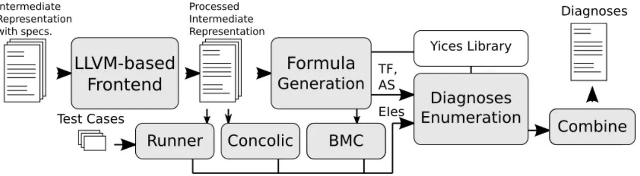
This thesis is organized as follows. Chapter 2 presents backgrounds of the fault localization of imperative programs. Chapter 3 introduces a series of concepts and terminologies that are needed to define the formula-based fault localization problem. These concepts and terminologies are used in the other chapters. Chapter 4 details the architecture of the tool SNIPER. The implementation of SNIPER, which is based on the LLVM compiler infrastructure and the Yices 1 partial maximum satisfiability solver, is detailed in Annex A. SNIPER is a basis on top of which we implement the different trace formulas presented in Chapters 5 and 7 and the algorithm of Chapter 6. In each of these chapters, we use SNIPER to empirically study the presented methods.
Chapter 5 introduces a method for encoding programs, the full flow-sensitive trace formula (FFTF), which is equivalent to the control flow graph of the target program. The FFTF with appropriate algorithms is successful in localizing root causes in multi- fault programs for at least two of the benchmarks we used. However, although the FFTF is expressive, it is not efficient in view of computing time. In the Chapters 6 and 7 we present methods to deal with this problem. Chapter 6 presents a fault localization algorithm, which enumerates minimal correction subsets (MCS) in an incremental fashion. We show on a benchmark that the computing time can be reduced with this algorithm. Chapter 7 introduces an alternative method for encoding programs, the hardened flow-sensitive trace formula (HFTF). We empirically show on two benchmarks that the use of the HFTF, as compared to the FFTF, makes the fault localization algorithm produce less spurious root causes and perform faster. The HFTF is shown to be as expressive as the FFTF for most programs. Finally, Chapter 8 summarizes the contributions of this thesis and presents a list of future work on formula-based fault localization of imperative programs.
Title Page . . . i
Abstract . . . iii
Table of Contents . . . vi
List of Figures . . . x
List of Tables . . . xi
Acknowledgments . . . xiv
1 Introduction 1 2 Backgrounds 4 2.1 Introduction . . . 4
2.2 Program Debugging . . . 5
2.3 Program Slicing . . . 6
2.3.1 Static Slicing . . . 6
2.3.2 Dynamic Slicing . . . 6
2.4 Coverage-based Fault Localization . . . 7
2.5 Counterexample Minimization . . . 9
2.6 Model-based Diagnosis . . . 9
2.7 Formula-based Fault Localization . . . 10
2.8 Program Fault Types . . . 10
2.8.1 Single-fault Programs . . . 12
2.8.2 Multi-fault Programs . . . 13
3 Preliminaries 17 3.1 Boolean Satisfiability Problem . . . 17
3.1.1 Basic Definitions . . . 17
3.1.2 Satisfiability and Unsatisfiability . . . 18
3.1.3 Maximum Satisfiability . . . 18
3.1.4 Partial Maximum Satisfiability . . . 19
3.2 Satisfiability Modulo Theories . . . 19
3.3 Bounded Model Checking . . . 20
3.4 Formula-based Fault Localization . . . 20
vi
3.4.1 MUS, MCS, Hitting Set, and MSS . . . 20
3.4.2 Root Causes . . . 22
3.4.3 Code Size Reduction . . . 22
3.4.4 Failing Program Paths . . . 23
3.4.5 Fault Localization Problem . . . 25
3.4.6 Example . . . 25
3.5 Static Single Assignment Form . . . 27
3.6 Program Dependence Graph . . . 30
4 Proposed Tool Architecture 33 4.1 Overview . . . 33
4.2 Program Encoding . . . 36
4.3 Test Cases Generation . . . 36
4.3.1 BMC Module . . . 37
4.3.2 Concolic Module . . . 38
4.3.3 Runner Module . . . 38
4.4 Diagnosis Enumeration . . . 39
4.4.1 Classic MCS Enumeration . . . 39
4.4.2 Basic Diagnosis Enumeration for Imperative Programs . . . . 42
4.4.3 Discussions . . . 42
4.5 Diagnosis Combination . . . 43
4.5.1 Flattening-based Combination . . . 44
4.5.2 Hitting-set-based Combination . . . 44
4.5.3 Union Pair-wise-based Combination . . . 45
4.5.4 Discussion and Related Work . . . 48
5 Full Flow-sensitive Trace Formula 50 5.1 Introduction . . . 50
5.2 Trace Formula Encodings . . . 51
5.3 Full Flow-sensitive Trace Formula . . . 52
5.3.1 Encoding of the Data Computation . . . 53
5.3.2 Encoding of the Control-Flow . . . 53
5.3.3 Whole Trace Formula . . . 54
5.3.4 Formula Granularity Level . . . 55
5.4 Fault Localization with FFTF and AllDiagnoses Algorithm . . . 57
5.5 Experiments on the TCAS Benchmark . . . 59
5.5.1 TCAS Benchmark . . . 59
5.5.2 Experimental Setup . . . 59
5.5.3 Results for Single and Multiple Faults . . . 60
5.5.4 Results with Different Formula Granularity Levels . . . 61
5.6 Experiments on the Bekkouche’s Benchmark . . . 63
5.6.1 Bekkouche’s Benchmark . . . 63
5.6.2 Results for Single and Multiple Faults . . . 63
5.6.3 SNIPER vs. BugAssist . . . 65
5.7 Discussion . . . 66
5.8 Summary . . . 68
6 Incremental Diagnosis Enumeration 75 6.1 Introduction . . . 75
6.2 Proposed Approach . . . 76
6.3 Experiments on the TCAS Benchmark . . . 77
6.3.1 Results . . . 77
6.4 Summary . . . 79
7 Hardened Flow-sensitive Trace Formula 80 7.1 Introduction . . . 80
7.2 Proposed Approach . . . 81
7.2.1 Hardened Flow-sensitive Trace Formula . . . 81
7.2.2 Calculating Hardened Flow-sensitive Trace Formula . . . 84
7.2.3 Fault Localization with Hardened Flow-sensitive Trace Formula 85 7.2.4 Example . . . 85
7.3 Experiments on the Bekkouche’s Benchmark . . . 87
7.3.1 Full Flow-sensitive TF vs. Hardened Flow-sensitive TF . . . . 87
7.4 Experiments on the TCAS Benchmark . . . 90
7.4.1 Experimental Setup . . . 90
7.4.2 Full Flow-sensitive TF vs. Hardened Flow-sensitive TF . . . . 90
7.5 Discussion and Related Work . . . 94
7.6 Summary . . . 95
8 Conclusion 97 8.1 Summary of the Thesis . . . 97
8.2 Future Work . . . 98
Bibliography 100 A Tool Implementation 109 A.1 LLVM Compiler Infrastructure . . . 109
A.1.1 Intermediate Representation Compilation . . . 110
A.2 Yices SMT Solver . . . 111
A.2.1 Application Programming Interface . . . 111
A.2.2 Incremental Assertions . . . 113
A.3 Program Parsing and Pre-processing . . . 113
A.3.1 Intermediate Representation Parsing . . . 114
A.3.2 Function Inlining . . . 114
A.3.3 Local Variables Processing . . . 116
A.3.4 Static Single Assignment Form Transformation . . . 117
A.3.5 Loops Processing . . . 117
A.3.6 Finalization . . . 121
B List of Publications 122 B.1 Journal Papers (refereed) . . . 122
B.2 International Conference Papers (refereed) . . . 122
B.3 Domestic Conference and Workshop Papers . . . 122
B.4 Awards & Honors . . . 123
2.1 A typical debugging process . . . 5
2.2 Fault types found in imperative programs . . . 15
3.1 Control flow graph of function foo . . . 24
3.2 The statement s2 is control-dependent on the statement s1 . . . 30
3.3 The statement s2 is data-dependent on the statement s1 . . . 31
3.4 A function and its PDG . . . 32
4.1 SNIPER tool flow . . . 33
5.1 Clause Enabling/Disabling . . . 58
5.2 Results of running SNIPER on the TCAS benchmark with different granularity levels for the FFTF . . . 62
5.3 A failing execution path . . . 67
5.4 Execution path after the clause B was relaxed . . . 67
6.1 Results of running SNIPER on the TCAS benchmark with and without push & pop optimization. . . 78
7.1 Control flow graph of function rotate (Listing 2.1) . . . 86
7.2 Results on Bekkouche’s benchmark with both types of encoding . . . 88
7.3 Results of running SNIPER on the TCAS benchmark with both types of encoding (part 1/2) . . . 91
7.4 Results of running SNIPER on the TCAS benchmark with both types of encoding (part 2/2) . . . 92
A.1 Frontend for LLVM . . . 110
A.2 A loop CFG in normal form . . . 119
A.3 From left to right, the steps to unroll a loop . . . 121
x
2.1 An example of data collected in coverage-based methods . . . 7 5.1 The types of trace formula used in formula-based fault localization and
their specificities (1/2) . . . 50 5.2 The types of trace formula used in formula-based fault localization and
their specificities (2/2) . . . 51 5.3 Results of SNIPER with the FFTF and BugAssist on the TCAS. Ver-
sions no. 33 and no. 38 are omitted from the table in order to compare the results with BugAssist [47], which does not have entries for them. For versions no. 4 and no. 41, a new option of SNIPER that checks the array index overflow/underflow can detect the missing fault. . . . 70 5.4 Types of Error in the TCAS programs . . . 71 5.5 Results of running SNIPER on the Bekkouche’s benchmark. . . 72 5.6 Results on the Bekkouche’s benchmark . . . 73 5.7 The types of trace formula used in formula-based fault localization and
their specificities . . . 74
xi
2.1 A single-fault program . . . 13
2.2 A multi-fault program infected by independent faults . . . 16
3.1 A function that returns a positive value at a given index, or zero if the index is negative . . . 23
3.2 A multi-fault program infected by two faults . . . 24
3.3 A function that computes an absolute value . . . 26
5.1 Code fragment from program Maxmin6varKO3 showing the two faults (underlined) . . . 64
A.1 Example of using the Yices API . . . 112
A.2 Loading and parsing of the input LLVM IR bitcode . . . 114
A.3 Forcing function inlining. . . 115
A.4 Function foo . . . 115
A.5 Before Inlining . . . 115
A.6 After Inlining . . . 115
A.7 Before processing. . . 116
A.8 After processing. . . 116
A.9 SNIPER inlining procedure. . . 116
A.10 Original Intermediate Representation . . . 117
A.11 Intermediate Representation in SSA form . . . 117
A.12 Transform a LLVM function into SSA form . . . 117
A.13 Unroll to a given bound all loops present in the target function . . . . 118
A.14 Loop before rotation . . . 119
A.15 Loop after lowering . . . 120
xii
A.16 Loop after rotation . . . 120 A.17 Assigning names to anonymous instructions . . . 121
My time as a graduate student at SOKENDAI and NII has been supported by many kind people. This page attempts to recognize those who have been most helpful along the way.
Firstly, I would like to express my sincere gratitude to my advisor Prof. Shin Nakajima for the continuous support of my Ph.D study and related research, for his patience, motivation, and immense knowledge. His guidance helped me in all the time of research and writing of this thesis. I could not have imagined having a better advisor and mentor for my Ph.D study.
Besides my advisor, I would like to thank the rest of my thesis committee: Prof. Hiroshi Hosobe, Prof. Kozo Okano, Prof. Ichiro Satoh, and Prof. Tomohiro Yoneda, for their insightful comments and encouragement, but also for the hard question which incented me to widen my research from various perspectives.
I thank my fellow labmates in for the stimulating discussions and for all the fun we have had in the last three years.
Last but not the least, I would like to thank my family: my parents and to my brothers and sister for supporting me throughout writing this thesis and my life in general.
xiv
xv
Introduction
As software-intensive systems constitute the social infrastructure to support our daily life, achieving the required reliability levels is a major concern in software en- gineering. In 1972, E.W. Dijkstra [27] discussed in his Turing awards lecture the importance of the correct by construction (CbyC) style development of programs. The presentation is a driving force of a wide variety of work in formal methods, espe- cially in the European research community. The idea is to construct correct programs from their initial formal specifications in a stepwise refinement manner. Correctness of the refinement is ensured in each step, and thus the resultant programs are correct. E.W. Dijkstra, actually, had a negative opinion on the effectiveness of a posteriori verification of programs. Although the idea of CbyC is scientifically sound, it is not adapted in practice. Constructing programs or programming is more or less a human process, requiring much experience and insight. The reliability of programs is also a matter of human activities.
Introducing some form of automation to a posteriori verification of programs is an alternative approach for achieving the required reliability levels. These methods adapt mathematical logic as their scientific bases. Software artifacts such as de- sign specifications or programs have their representations encoded as logic formulas. Correctness of programs with respect to the given specifications is a process of math- ematical reasoning. This can be automated when formulas are in decidable fragments of first-order theory. In particular, with the advent of the efficient Boolean satisfia-
1
bility (SAT) technology [74], SAT-based methods occupy one of the central themes in automated software engineering. These are applying SAT to automatic test-case generations or bounded model checking of programs [20, 21, 41, 51, 66]. They are effective in checking whether the target program is faulty or not. Identifying root causes of the faulty behavior still needs a vast amount of human efforts. Localizing root causes automatically is now an important research challenge.
Automatic fault localization is formulated as a problem of mathematical logic. R. Reiter [77] introduced the model based diagnosis (MBD) theory. In the MBD theory, the model of the artifact is encoded in a formula of some suitable logic. The model together with a given specification is unsatisfiable if the artifact is faulty. The problem is to find a set of clauses in the artifact model that are responsible for this unsatisfiability. If the formula is encoded in Boolean, it is exactly an in- stance of Boolean unsatisfiability problem (UNSAT). As the complexity of UNSAT is coNP-complete, M.H. Liffiton et al. [59] turns it into a dual problem of maximum satisfiability (MaxSAT) whose complexity is NP-complete [12]. R. Reiter’s framework and M.H. Liffiton’s work are successful in the fault localization of VLSI circuit de- signs [80] together with efficient MaxSAT algorithms. Similar methods are employed in the fault localization of imperative programs, but they are limited to programs with a single fault in them [47, 95]. There is a need for a new method to identify multiple faults in a program.
This thesis presents a new automatic fault localization method for programs that have multiple faults in them. The method adapts a modest assumption on the failure model of imperative ANSI C programs. The key observation is the way to encode all the potential failing execution paths in a logic formula, called trace formula (TF). The TF encodes the failure model as well as those potential failing execution paths, and thus has much impact on the preciseness and efficiency of localizing faults. The proposed method is implemented in a tool, SNIPER. In some experiments on typical benchmark problems, SNIPER successfully identifies all the injected, both single and multiple faults. These experiments show that the assumption of the failure model is adequate at least for the benchmark problems used, and the fault localization is efficient.
The organization of the thesis is as follows. Chapter 2 presents backgrounds of the fault localization of imperative programs. Chapter 3 introduces a series of con- cepts and terminologies that are needed to define the formula-based fault localization problem. These concepts and terminologies are used in the other chapters. Chap- ter 4 details the architecture of the tool SNIPER. The implementation of SNIPER, which is based on the LLVM compiler infrastructure and the Yices 1 partial maximum satisfiability solver, is detailed in Annex A. SNIPER is a basis on top of which we implement the different trace formulas presented in Chapter 5 and 7 and the algo- rithm of Chapter 6. In each of these chapters, we use SNIPER to empirically study the presented methods. Chapter 5 introduces a method for encoding programs, the full flow-sensitive trace formula (FFTF), which is equivalent to the program’s control flow graph. The FFTF with appropriated algorithms is successful in localizing root causes in multi-fault programs for at least two of the benchmarks we used. However, because the FFTF is expressive, it is not efficient in view of computing time. In the Chapter 6 and 7 we present methods to deal with this problem. Chapter 6 presents a fault localization algorithm, which enumerates minimal correction subsets (MCS) in an incremental fashion. We show on a benchmark that the computing time can be reduced with this algorithm. Chapter 7 introduces an alternative method for en- coding programs, the hardened flow-sensitive trace formula (HFTF). We empirically show on two benchmarks that the use of the HFTF, as compared to the FFTF, makes the fault localization algorithm produce less spurious root causes and perform faster. Finally, Chapter 8 summarizes the contributions of this thesis and presents a list of future work on formula-based fault localization of imperative programs.
Backgrounds
This chapter introduces backgrounds of the automatic fault localization of imper- ative programs, and summarizes related work.
2.1 Introduction
In the world of software development, software reliability [73] is of a great im- portance, however, it is rather immature in general. “Software reliability is the probability of failure-free operation of a computer program for a specified time in a specified environment [71]”. E.W. Dijkstra believed that program reliability would be achieved by finding a way to avoid writing programs with bugs from the very beginning [27]. Such a way would make the programming process cost effective since software engineers would not waste their time in debugging programs. Correct by construction (CbyC) style development is one such approach. For example, the ver- ification method [64] helps in assisting the development of software and hardware systems. The program is refined in a stepwise manner, starting from its formal spec- ification, and ending with actual code. Therefore, the correctness at each refinement step is preserved. However, formal specifications are difficult to apply in practice because of their very limited expressiveness compared to the Natural language. It requires a big effort to use and understand the notation for software engineers.
Even though the idea of CbyC was attracting, posteriori verification became a
4
standard in recent years. The focus changed from product over process and the goal is now to detect faults after the code is developed. Thus was born the activity of program debugging, which aims at improving software reliability.
2.2 Program Debugging
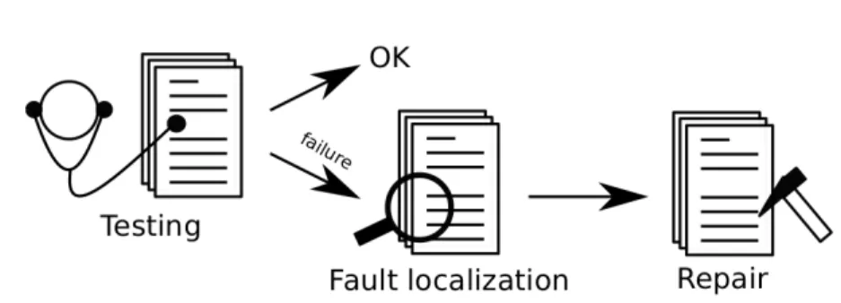
Figure 2.1: A typical debugging process
Program debugging is a complex activity that involves several tasks. As illustrated in Figure 2.1, debugging starts by testing a target program to see if it is faulty or not. Testing can be done manually or automatically. There exist various automatic tech- niques, including program testing or automatic formal verification. Once the testing phase is finished and in the case the target program exhibits inappropriate behavior (i.e., failures), the next task consists of identifying the reasons of the failures. This task is called fault localization. Fault localization can be time-consuming and difficult especially when done manually. Once the reasons of the failures are successfully iden- tified and their root causes are localized, they need to be corrected. Fault repair aims at repairing the faults previously identified. The process of debugging ends when the target program behaves as expected.
Three of the debugging tasks are closely related and can strongly influence each other. A good testing result is important for making the fault localization task easy to perform. Similarly, fault reports generated by the fault localization task must contain enough information to facilitate and speed up the fault repair task.
In the present thesis, we focus on the task of automatic fault localization. In the following sections, we present existing approaches to tackle the problem of fault
localization in imperative programs.
2.3 Program Slicing
Program slicing [88, 89, 90] is a technique for analyzing imperative programs, which can be used in debugging to locate root causes of errors. Program slicing consists of finding the instructions of a program that can affect a variable v at a line l, a slicing criterion. The subset of instructions obtained from the whole program is called a slice. A slice is defined with respect to a slicing criterion. If the slicing criterion refers to a violation of an assertion, then the obtained slice is a subset of program statements that directly affect the assertion violation. Thus, the slice contains root causes. Further, we sometimes say a failing slicing when a slice of code contains faults. Similarly, a slice of code that does not contain faults is called a successful slice.
Program slicing for localizing faults was empirically shown effective [52]. The average code size reduction (CSR) of program slices is around 30% [13]; such amount of program code needs to be inspected manually to find real root causes.
2.3.1 Static Slicing
According to the original definition of slicing [89], a static slice of a program P is all statements of P that may affect the value taken by a variable v at a point p of the program. This slice is defined for a slicing criterion C = (s, V ), where s is a statement of the program P and V is a subset of variables in P . Computing a static slice consists of finding successive sets of statements that are indirectly pertinent, in accordance with data and control dependencies.
2.3.2 Dynamic Slicing
Dynamic slicing is similar to static slicing but instead it uses information obtained at execution time. A dynamic slice contains all statements that actually affect the value of a variable at a program point for a particular program execution. A static
slice would contain all statements that may have affected the value of a variable at a program point for any program execution.
With dynamic slicing the produced slices are usually smaller than with static slicing. This is because static slicing methods do not make any assumptions regarding program inputs. Whereas a dynamic slice contains only the program statements that are dependent on specific program inputs.
2.4 Coverage-based Fault Localization
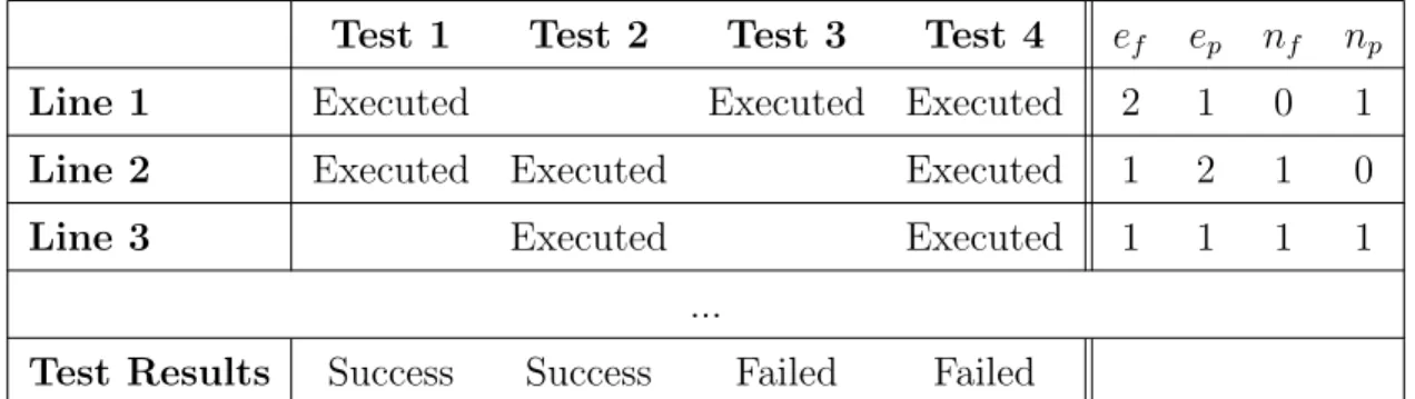
Coverage-based or spectrum-based debugging [45, 46, 78, 91] calculates ranking orders between program statements or spectrums to show that a particular fragment of code is more suspicious than the others. The method needs many successful and failing executions to calculate the statistical measures. The method basically relies on program testing technique, and needs input-output test data. Generating unbiased test data set is a major challenge.
The method consists of collecting data while executing the program in order to determine the potential root cause locations. The data can be collected at different spectrum, such as: line, block, function, class, or packet.
Example
Test 1 Test 2 Test 3 Test 4 ef ep nf np
Line 1 Executed Executed Executed 2 1 0 1
Line 2 Executed Executed Executed 1 2 1 0
Line 3 Executed Executed 1 1 1 1
...
Test Results Success Success Failed Failed
Table 2.1: An example of data collected in coverage-based methods
In the example of Table 2.1, the Line 1 is executed by the Tests 1, 3, and 4. Two of these tests failed (ef) and one succeeded (ep). All the failed tests were executed
on this line (nf) and one successful test does not execute this line (np). The Line 2 is executed by Tests 1, 2, and 4. One of these tests failed (ef) and two succeeded (ep). One failed test does not execute this line (nf) and all the successful tests execute this line (np).
Metrics
Metrics allow to calculate a Hamming distance between code entities (line, block, function, class) and a bug. There exists many different metrics. The entities can be sorted depending on the distance, the nearest ones from the bug contain the most probable the bug, and the farthest ones are probably not causing the bug. Based on this sorting, software engineers can find faster the source of the error than a manual search.
Tarantula
Tarantula is a metric but also a tool introduced by Jones et al. [45]. Tarantula is representative of the coverage-based approach. It was developed in order to provide a standalone tool for the visualization of program lines of code. The studied lines of code are colored depending on their suspiciousness. In addition to the color, varying from green for not suspected lines to red for suspected lines, a shade shows the number of time the lines where effectively executed by the test suite. These two information are combined in order to produce a display that shows the degree of suspiciousness associated to each line.
Tarantula can be greatly affected by the test data used, and this is also true for all methods following the coverage-based approach. In the experiment sections of Chapter 5 and Chapter 7 we show two cases on which Tarantula is unable to find the faults. The reason is that Tarantula is using statistics to compute the root cause locations. Depending on the provided test data (test-cases) but also the types of faults in the target program, the method may or may not find the faults. We discuss the types of faults in more details in Section 2.8.
2.5 Counterexample Minimization
Model checking methods are used to automatically check whether a target artifact is faulty or not. When the target artifact is shown to be faulty, a model checking methods outputs a counterexample. It requires a great amount of manual efforts to identify root causes by studying the generated counterexamples. Counterexample minimization [6, 16, 37, 38] is introduced to help this task.
Counterexample minimization methods are used together with logic model check- ing. Fault localization methods based on counterexample minimization attempts to reduce the number of irrelevant part of a counterexample. Informally, the error lo- calization is a problem of finding fragments of the program that appear in the error traces, but not in the successful executions. This observation leads to the auto- mated methods to calculate how the error traces are different from the successful ones [6, 16, 37, 38]. Alternatively, some work views the problem as minimizing the error traces, namely to find a set of minimal lengths in the traces to result in the failing executions [17, 47].
2.6 Model-based Diagnosis
The model-based diagnosis (MBD) theory [36, 77] establishes a logical formalism of the fault localization problem. The model is presented as a formula expressed in suitable logic. The formula is unsatisfiable if it represents both an artifact and a correctness criteria, with the former violating the latter. The MBD theory dis- tinguishes conflicts and diagnoses. Conflicts are the erroneous situations similar to failing static slicing (see Section 2.3.1), and are represented by minimal unsatisfiable subsets (MUSes) of the unsatisfiable formula. Diagnoses are the fault locations to be identified and are minimal correction subsets (MCSes). The MBD theory states that MUSes and MCSes are connected by the hitting set relationship. Therefore, the problem is to enumerate either all MUSes or all MCSes. Such sets can be calculated automatically if the formula is represented in decidable fragments of first-order theory, for example, as a Boolean formula. If the formula is encoded in Boolean, the problem
becomes a Boolean unsatisfiability problem (UNSAT). Note that the complexity of UNSAT is coNP-complete [12].
The MBD methods, including the model-based debugging [95], first calculate MUSes and then obtain MCSes. There are several ways to calculate the information equivalent to MUSes. An early work [93] used graph-based algorithms to compute a static slice of programs in order to obtain MUSes. Later, MUSes were obtained by calculating irreducible infeasible subsets of constraints [95].
2.7 Formula-based Fault Localization
Formula-based fault localization method combines the SAT-based formal verifica- tion techniques [74] with the model-based diagnosis (MBD) theory [77]. This method was first employed in the fault localization of VLSI circuits [80] as an alternative approach to obtaining the minimal correction subset (MCSes). The method reduces the fault localization problem to maximum satisfiability of unsatisfiable formulas in propositional logic and calculates maximal satisfiable subsets (MSSes). An MCS is the complement of MSS [60]. Therefore, the problem is turned into a dual problem of maximum satisfiability (MaxSAT) whose complexity is NP-complete [12].
This idea was applied to the fault localization problem of imperative programs [47] and implemented in a tool, BugAssist. The algorithm of BugAssist, however, does not guarantee the enumeration of all the MSSes. It may miss some faults, especially in programs with multiple-faults.
In summary, the formula-based approach is more systematic than the methods that use program slices (Section 2.3) or the statistical coverages (Section 2.4). It has its logical foundation developed in the MBD theory (Section 2.6).
2.8 Program Fault Types
In this section we explain the notion of faults in imperative programs. We provide insights on the different types of faults and on their characteristics.
In debugging of imperative programs, bugs or defects can be divided into the following categories.
1. Syntax: invalid sequence of characters or tokens, 2. Data Size: arithmetic overflow or underflow,
3. Sanity: buffer overflow, null pointer, division by zero, 4. Application Features .
The formula-based fault localization focuses on faults related to (4) application features. Other categories of defects are not considered here. Application features are usually specified by assertions in the code, or by a design-by-contract (DbC) style specification [41, 67, 68, 69] (pre- and post-conditions, and invariants).
Application feature faults can be further divided into two categories. The first category refers to faults in the calculations. Typically, these faults occur when the software engineer makes a mistake in using a comparison/arithmetic operator. The second category refers to faults in the structure of the program. The structure, also called skeleton, is usually defined by the way program basic blocks are interconnected to each other. In some situations, this skeleton is incorrect and thus making the program not behave as expected. Automatic fault localization methods, introduced so far (Section 2.2 to 2.6), consider calculation faults only. Herein we also assume that the structure or skeleton of the target program is correct, and we focus on calculation faults.
Some faults are seeded in existing lines of code that were not properly written. Other faults are caused by missing fragments of code (omissions). The latter is especially difficult to deal with because we have to localize a part of non-existing code fragments. In this thesis we focus on the former and do not consider fault due to omissions.
Now, we will discuss in what kind of programs our method will look for root causes of faults. The classification of imperative programs is made according to the number of faults they are infected with. The following two sections details the types of programs to be considered.
2.8.1 Single-fault Programs
A single-fault program is a program that contains only one fault. The fault is either a wrong comparison operator, for example in an if-statement, or a wrong operator in an arithmetic operation.
Usually, to debug a single-fault program, a single error-inducing input is enough to find out root causes of the fault. This error-inducing input triggers a failing path on which the fault is executed. All the fault localization methods, mentioned in Section 2.3 to 2.7, are effective for such single fault-programs. However, usually, we may have many different error-inducing inputs. Imagine that we have a test suite consisting of many test cases and a target program that has a single fault. There are some cases where some of the test cases fail on the program. The other test cases are passed. This happens if the particular fault can be reached in many different execution paths. The coverage-based fault localization methods, in particular, rely on the existence of such test cases.
Example
We illustrate the problem of fault localization on single-fault programs with an example in Listing 2.1. This program is supposed to compute two values to operate a motor. The first value (d) is meant for giving the order to torque, turn right, or turn left to the motor. The second value is a positive or null number representing the rotation degree. However, there is an error in this program, which is located in line 11. The comparison (d==1) should be (d==2). Because of this error, when putting as argument to the procedure rotate a non-null number, the assert in line 16 fails because the value of r is negative. Hence, an error-inducing input equal to 1 or −1 can be used to trigger a failing execution.
1 void r o t a t e ( int d e g r e e ) { 2 i n t d ;
3 i f ( d e g r e e ==0) { 4 d = 0 ; // t o r q u e 5 } e l s e i f ( d e gr e e >0) { 6 d = 1 ; // r o t a t e r i g h t 7 } e l s e {
8 d = 2 ; // r o t a t e l e f t
9 }
10 i n t r ; 11 i f ( d==1) {
12 r = d e g r e e ∗ −1; 13 } e l s e {
14 r = d e g r e e ;
15 }
16 a s s e r t ( 0 <= d <= 2 && r >= 0 ) ; 17 opMotor ( r , d ) ;
18 }
Listing 2.1: A single-fault program
2.8.2 Multi-fault Programs
Dealing with programs with multiple faults is one of the important issues in au- tomated fault localization methods. As mentioned before, most of the current fault localization approaches focus on single-fault programs and are not effective for multi- fault programs. We, here, focus on the coverage-based methods. Coverage-based debugging methods are unable to locate multiple faults simultaneously. This was empirically studied by DiGiuseppe et al. [26]. They showed that the presence of multiple faults caused interferences, which inhibits the effectiveness of the method. It is, however, true that at least one fault can be localized. Denmat et al. state that the coverage-based technique Tarantula [46] makes implicit hypotheses requir- ing independence of multiple faults (every failure is caused exclusively by a single fault) and when these hypotheses do not hold, the technique does not provide “good
result” [25]. Zheng et al. assert that traditional coverage-based technique “cannot distinguish between useful bug predictor and predicates that are secondary manifes- tations of bugs” [99].
The MBD theory [77] generally considers the multiple fault cases. For simplicity, consider a case where a set M of MUSes is extracted from an unsatisfiable formula and each MUS in M refers to a particular error, a single fault. Then, M may contain, in principle, many conflicts because many elements (clauses) are included. MCSes, calculated using the minimal hitting set of MUSes, contain elements (clauses) repre- senting multiple faults.
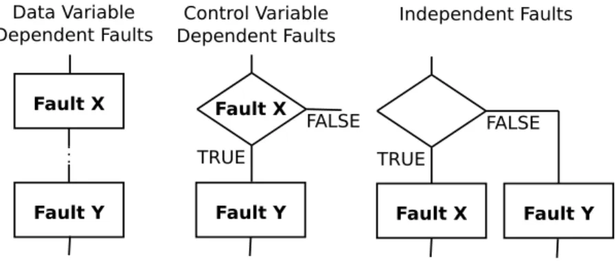
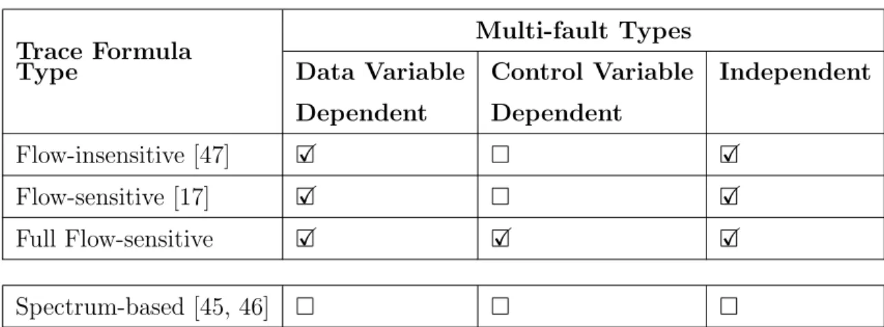
In order to study the characteristics of multiple faults in detail, we classify the types of faults that can be found in multi-fault programs in three categories:
• Data flow-dependent faults
• Control-dependent faults
• Independent faults
Figure 2.2 depicts an example of control flow graph (CFG) for each of the above types of faults. Informally, a faulty statement Y is data flow-dependent on a faulty statement X if the result of Y is dependent on X. A faulty statement Y is control- dependent on a faulty branch condition X of a conditional branch statement if the outcome of X determines whether Y should be executed or not. In a special case of the control-dependent faults, the fault X may hide the fault Y , which means that it is impossible to generate a test case that executes the fault Y and detects the existence of Y . We call such special case, nested faults. Lastly, a faulty statement Y is independent of a faulty statement X if Y and X are neither control-dependent nor data flow-dependent.
In some cases, multiple faults can lie in one program path. In such a situation, a single test input is enough to localize all the faults. In some cases of data flow- dependent faults or control-dependent faults, the use of full flow-sensitive TF can sometimes locate different faults with a single test input. We will discuss this later in regard to the Bekkouche’s Benchmark (Section 5.6.1).
FALSE TRUE
Fault X Fault Y FALSE
TRUE Fault X
Fault Y
Independent Faults Control Variable
Dependent Faults
Fault Y Fault X Data Variable Dependent Faults
Figure 2.2: Fault types found in imperative programs
When faults are independent, it usually requires to have multiple test inputs in order to successfully identify all faults. Additionally, if faults are localized in different failing paths, a method to combine the results obtained from these paths is needed in order to show to the programmers that there are more than one fault to look at in the faulty programs. A basic MCS enumeration method that uses a single failing test case only is not sufficient when dealing with multi-fault programs whose faults are spread in different program paths or execution paths. In Chapter 4 we introduce an MCS enumeration method and a combination method that are, when used together, suited to tackle this special case of multi-fault programs.
Example
We illustrate the problem of multi-fault program with an example shown in List- ing 2.2. This program contains two faults. In line 4 the variable y should be set to 42 and in line 6 it should be set to 0. We can find two failing paths, one that goes through the line 4 with the value 1 as argument, and the other that goes through the line 6 with the value 0 as argument. We are faced with two problems with this kind of program. First, we need to take into account both failing paths to localize all the faults. Considering only one path is not sufficient. Second, the quantity of faults in the program may affect the precision of the fault localization because the cause of an erroneous situation can be due to one or many faults acting together. An accurate localization implies an high complexity of analysis.
1 void f o o 1 ( int x ) { 2 i n t y ;
3 i f( x>0) {
4 y = 1 ; // F a u l t X
5 } e l s e {
6 y = 4 2 ; // F a u l t Y
7 }
8 a s s e r t ( ( x<=0 && y==0) | | ( x>0 && y==42) ) ; 9 }
Listing 2.2: A multi-fault program infected by independent faults
Preliminaries
This chapter introduces a series of concepts and terminologies, which are manda- tory for understanding the remaining part.
3.1 Boolean Satisfiability Problem
Boolean satisfiability problem (SAT problem) is a decision problem defined with logic formulas. It is, given a formula in propositional logic, to decide if this formula has a model, meaning that if there exists an assignment of the propositional variables making the formula true.
3.1.1 Basic Definitions
Clause
A clause is a disjunction of literals. In propositional logic, a clause takes the form (l1∨ ... ∨ ln)
where li are literals; an atomic proposition (p) or a negation of an atomic proposition (¬p).
17
Conjunctive Normal Form
A formula in conjunctive normal form (CNF) is a normalization of a logical ex- pression, which is a conjunction of clauses.
3.1.2 Satisfiability and Unsatisfiability
Satisfiability and validity are elementary concepts of semantics. A formula is satisfiable if it is possible to find an interpretation (model) that makes the formula true. A formula is valid if for all interpretations the formula is true. Dual concepts are the unsatisfiability and the non-validity. A formula is unsatisfiable if none of its interpretations makes the formula true, and non-valid if it exists an interpretation that makes the formula false.
The four concepts can be applied to theories. A theory is a set of sentences in a formal language. For example, a first-order theory is a set of first-order sentences. A theory is satisfiable (valid) if one (or all) interpretations make each axiom of the theory true, and the theory is unsatisfiable (non-valid) if all (one) interpretation make each axiom of the theory false.
It is also possible to consider only interpretations that make all of the axioms of another theory true. This generalization is commonly called satisfiability modulo theories (see Section 3.2 for details).
The question whether a sentence in propositional logic is satisfiable is a decid- able problem, which is a question in some formal system with a yes-or-no answer, depending on the values of some input parameters. In general, the question whether sentences in first-order logic are satisfiable is not decidable.
3.1.3 Maximum Satisfiability
The maximum satisfiability (MaxSAT) problem is the problem of determining the maximum number of clauses, of a given Boolean formula in CNF, that can be made true by an assignment of truth values to the variables of the formula. It is a generalization of the Boolean satisfiability problem, which asks whether there exists
a truth assignment that makes all clauses true. For example, the CNF formula
ϕ = (a ∨ b) ∧ (a ∨ ¬b) ∧ (¬a ∨ b) ∧ (¬a ∨ ¬b)
is not satisfiable, which means that no matter which truth values are assigned to its two propositional variables, at least one of its four clauses will be false. However, it is possible to assign truth values in such a way as to make three out of four clauses true; indeed, every truth assignment will do this. Therefore, if this formula is given as an instance of the MaxSAT problem, the solution to the problem contains three clauses.
3.1.4 Partial Maximum Satisfiability
In the partial maximum satisfiability (pMaxSAT) problem for a CNF formula, some clauses are declared to be soft, or relaxable, and the rest are declared to be hard, or non-relaxable. The problem is to find an assignment that satisfies all the hard clauses and the maximum number of soft clauses.
For example, consider again the example CNF formula in the previous section, but this time with its clauses assigned as soft or hard:
ϕpartial = (a ∨ b) ∧ (a ∨ ¬b) ∧ (¬a ∨ b)
| {z }
sof t
∧ (¬a ∨ ¬b)
| {z }
hard
One solution is to retract the clause (a ∨ b). We then obtain the following assignment: a= true and b = false.
3.2 Satisfiability Modulo Theories
The satisfiability modulo theories (SMT) [29] problem is a decision problem for logical formulas, with respect to combinations of background theories expressed in decidable subclass of first-order logic with equality. It is a generalization of a Boolean SAT instance in which various sets of variables are replaced by predicates from a
variety of underlying theories. Examples of theories are the theory of real numbers, the theory of integers, and the theories of various data structures such as lists, arrays, or, bit vectors.
3.3 Bounded Model Checking
Model checking [18, 75] is a set of techniques for automatic verification of systems. The principle is to algorithmically check if a given model, which can be the given system or an abstraction of the system, satisfies a specification often formulated in terms of temporal logic.
Model checking tools face a combinatorial blow up of the state-space, commonly known as the state explosion problem, that must be addressed to solve in cases of real- world problems. Bounded model checking (BMC) [9, 10, 11] is one of the approaches to combatting this problem. BMC algorithms [21, 20, 66] unroll the finite state machine to a fixed number of steps k and check whether a property violation can occur in k or fewer steps. This typically involves encoding the restricted model as an instance of SAT problem. The process can, in principle, be repeated with large values of k until all possible violations have been ruled out.
3.4 Formula-based Fault Localization
This section provides basic definitions on formula-based automatic localization method. Definitions of the basic concepts such as MUS, MCS, MSS, and hitting set, are found in the literature (cf. [60]).
3.4.1 MUS, MCS, Hitting Set, and MSS
In the following definitions, C is a set of clauses, which constitutes a CNF for- mula ϕ. We use C and ϕ interchangeably. Note that in this thesis we sometimes present a set of clauses as a set of line numbers. These line numbers refer to program statements (instructions) in the target source code. Since in our work clauses are
encoded from instructions, for sake of clarity we show the line numbers instead of the associated clauses.
Definition 1 (Minimal Unsatisfiable Subset) M ⊆ C is a Minimal Unsatisfi- able Subset (MUS) iff M is unsatisfiable and ∀c∈M :M \{c} is satisfiable.
Definition 2 (Minimal Correction Subset) M ⊆ C is a Minimal Correction Subset (MCS) iff C\M is satisfiable and ∀c ∈ M : (C\M ) ∪ {c} is unsatisfiable. An MCS is a set of clauses such that C can be corrected by removing an MCS from C. Therefore, an MCS is considered to represent a root cause.
Definition 3 (Hitting Set) H is a hitting set of Ω iff H ⊆ D and ∀S ∈ Ω : H∩ S 6= ∅.
Let Ω be a collection of sets from some finite domain D, a hitting set of Ω is a set of elements from D that covers (hits) every set in Ω by having at least one element in common with it. A minimal hitting set is a hitting set from which no element can be removed without losing the hitting set property. There exist many algorithms to compute the hitting set, such as those presented in [36, 77] or in [81, 82]. We show one algorithm for computing the minimal hitting set in Section 4.5.2.
Definition 4 (Maximal Satisfiable Subset) M ⊆ C is a Maximal Satisfiable Sub- set (MSS) iff M is satisfiable and ∀c ∈ C\M : M ∪ {c} is unsatisfiable.
By definition, an MCS is the complement of an MSS (MSS∁) [60].
Any solution to MaxSAT problem is also an MSS. However, every MSS is not necessarily a solution to MaxSAT [70].
We illustrate the above definitions with an example taken from [59]. Below, a CNF formula and its MSSes, MCSes and MUSes.
ϕ =(a) ∧W (¬a) ∧X (¬a ∨ b) ∧Y (¬b)Z MSSes(ϕ) = {{X, Y, Z}, {W, Z}, {W, Y }}
MCSes(ϕ) = {{W }, {X, Y }, {X, Z}} MUSes(ϕ) = {{W, X}, {W, Y, Z}}
To calculate the MSSes of ϕAL we use partial maximum satisfiability method.
3.4.2 Root Causes
In fault localization, the faults are identified by localizing their root causes. A root cause is the fundamental reason for the occurrence of a failing program execution. In the MBD theory, a root cause is represented by an MCS, and multiple root causes by MCSes. In practice, root causes help the programmers fix buggy programs. We conceptually distinguish real root causes and spurious root causes. Real root causes are program fragments that correct the program completely or partially when they are appropriately modified. In contrast, spurious root causes are program statements that when modified or removed do not fix the program with regard to the programmer’s intention. In this thesis, we sometimes refer to either real root causes or spurious ones, but such distinction is concerned with the so-called high-level design decision of programmers. They are not distinct in view of the fault localization algorithm. In particular, the injected faults in the benchmark problems (Sections 5.5, 5.6, 7.4 and 7.3) are considered real root causes.
3.4.3 Code Size Reduction
Code size reduction (CSR) is the ratio of fault locations in an MUS (a program slice) to the total number of lines of code. The CSR is calculated as follows:
csr(MUS ) = |MUS |
total number of lines
For example, in Listing 3.1 if we obtain the MUS M = {3, 4} with its elements being line numbers. The CSR for M is as follows:
csr(M ) = |M | ∗ 100
total number of line =
2 ∗ 100
10 = 20%
Note that using static slicing results in CSR to be around 30% [52]. Another common terminology for quantifying the ratio of fault locations is the average CSR (ACSR), which represents the CSR for a set of MUS. For a given set S of MUSes, the ACSR is calculated as follows:
acsr(S) = P
icsr(Si)
|S|
1 int getAt ( int ∗a , int x ) { 2 i n t y ;
3 i f ( x>=0) { 4 y = a [ x ] ; 5 } e l s e {
6 y = 0 ;
7 }
8 a s s e r t ( y>=0) ; 9 return y ; 10 }
Listing 3.1: A function that returns a positive value at a given index, or zero if the index is negative
3.4.4 Failing Program Paths
Let ϕAL be a formula in conjunctive normal form (CNF) such that ϕAL= ϕTI ∧ ϕTF ∧ ϕAS
where ϕTI is a formula that encodes the test inputs, ϕTF is a trace formula that encodes all the possible program execution paths up to a certain depth, and ϕAS is a formula that encodes the assertion that the program must satisfy. The detailed representation of TF is irrelevant here, and will be introduced in Chapter 5 and 7. The formula ϕAS can be the post-condition or test oracle. When program paths are failing, ϕTI represents the input arguments that take certain particular values, making ϕTF violate ϕAS. We call such ϕTI error-inducing (EI). There are several approaches to generating such failing test inputs. Bounded model checking (BMC) [21] is one such approach, which generates a counterexample from which a single failing test input can be extracted. Test case generation methods, such as concolic execution [33, 84], can generate more than one test case for a given program. Generated test data, that result in failing execution, constitute such EI.
Example
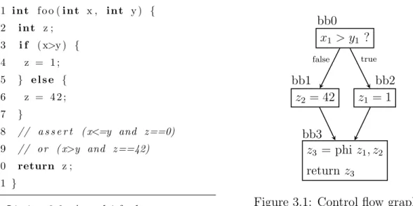
We introduce a simple program in Listing 3.2 and its CFG in Figure 3.1. List- ing 3.2 shows a function that takes two arguments. This program contains two faults. In line 4 the variable z should be set to 42 and in line 6 it should be set to 0. These two statements are called root causes.
1 int f o o ( int x , int y ) { 2 i n t z ;
3 i f ( x>y ) { 4 z = 1 ; 5 } e l s e { 6 z = 4 2 ;
7 }
8 // a s s e r t ( x<=y and z==0) 9 // or ( x>y and z ==42) 10 return z ;
11 }
Listing 3.2: A multi-fault program infected by two faults
x1 > y1 ? bb0
false true
z2 = 42 bb1
z1 = 1 bb2
z3 = phi z1, z2
return z3
bb3
Figure 3.1: Control flow graph of function foo
For program of Listing 3.2, we obtained the two failing test cases (error-inducing inputs) below.
ϕfooTI1 = (x1 = 1) ∧ (y1 = 0) ϕfooTI2 = (x1 = 0) ∧ (y1 = 1)
The post-condition of the function foo is encoded from the assertion of line 8 and takes the following form:
ϕfooAS = ((x1 ≤ y1) ∧ (z3 = 0)) ∨ ((x1 > y1) ∧ (z3 = 42))
The trace formula is encoded from lines 2 to 7. Its encoding is shown later in Sec- tion 5.3.
3.4.5 Fault Localization Problem
Since ϕAL encodes failing program paths with EI , the formula ϕAL is unsatisfi- able. By definition, EI and AS are supposed to be satisfied. The trace formula TF is responsible for the unsatisfiability. It is exactly the situation that the program con- tains faults. The fault localization problem is to find a set of clauses in TF that are responsible for the unsatisfiability. Such clauses are found in minimal unsatisfiable subsets (MUSes) of ϕAL. MUSes of the unsatisfiable formula are erroneous situations (conflicts) similar to failing static slicing (see Section 2.3). However, finding root causes in lengthy slices is difficult because many statements are included. According to the MBD theory [77], such root causes are diagnoses and are represented as MCSes. An important point in the fault localization problem is the number of test cases being used. Usually, one test case may be enough to identify an erroneous situation caused by a single fault. Lots of test cases are needed to show the existence of all multiple faults. It implies that we check the unsatisfiability of ϕAL(EIi) with many different EIi. A single counterexample approach does not work well for a general case of programs with multiple faults.
The fault localization problem is to find MCSes of ϕAL. The formula-based method adapted in herein [53] first calculates MSSes of ϕAL and then obtain MCSes by taking the complements of MSSes. Enumerating all the MCSes is mandatory to cover all the root causes.
3.4.6 Example
We explain the above concepts on the program of Listing 3.3. In line 6, there is an error in the computation of the absolute value of x in abs. The variable abs is equal to x*1 when x is negative, which violates the assertion at line 8 which expects abs to be greater or equal to zero.
1 int absValue ( int x ) { 2 i n t abs ;
3 i f( x>=0) {
4 abs = x ;
5 } e l s e {
6 abs = x ∗ 1 ; // s h o u l d be : a b s=x ∗ −1;
7 }
8 a s s e r t ( abs >=0) ; 9 return abs ; 10 }
Listing 3.3: A function that computes an absolute value
A failing trace can be obtained with an input value equal to -1. The error-inducing input extracted from the failing trace is encoded in EI and takes the following form: EI = (x0 = −1). The static single assignment (SSA) form of the function body (lines 2 to 7) is encoded in TF , as shown below. For recall, SSA form is a relation on program variables, which requires that each variable is assigned exactly once, and every variable is defined before it is used. Further details on the SSA form can be found in Section 3.5. See Section 5.3.4 concerning the mapping of clauses in TF to the original program statements. The assertion in line 8 is encoded in AS as follows: AS = (abs3 ≥ 0).
TF = (guard0 = (x0 ≥ 0))
| {z }
line 3
∧ (abs1 = x0)
| {z }
line 4
∧ (abs2 = x0× 1)
| {z }
line 6
∧
((guard0∧ (abs3 = abs1)) ∨ (¬guard0 ∧ (abs3 = abs2)))
| {z }
line 3
We obtain two MSSes and two MCSes, as shown below. The set elements represent the line numbers of the program in Listing 3.3. We create a set containing the two MCSes. The minimal hitting set of the resulting set gives us a set containing two MUSes, which are the conflicts:
MSS0 = {6} MCS0 = MSS∁0 = {3, 4} MSS1 = {3, 4} MCS1 = MSS∁1 = {6}
MCSes = {MCS0,MCS1} = {{3, 4}, {6}} MUSes = MCSesMHS = {{4, 6}, {3, 6}}
We here obtained two diagnoses; one with the line numbers 3 and 4, another with 6. The diagnosis {3, 4} indicates that both lines 3 and 4 should be corrected at a time. For example, if we change the statement in line 3 to be x<0 and the statement in line 4 to be abs=-x then, for the input x=-1, the program becomes correct. The diagnosis {6} indicates that line 6 only has to be modified to correct the program for the input x=-1. Software engineers are free to choose between these two diagnoses. From the diagnoses, we obtain two conflicts; one with the line numbers 4 and 6, another with 3 and 6. If we only need a set of potential root causes, we may extract the line numbers from either MCSes or MUSes to have a set, for example, {3, 4, 6}. The results are the same regardless of using MCSes or MUSes since only the line numbers are significant. It is what BugAssist [47] does to calculate the CSR. Note that with such a combination method, it is difficult, especially in the case of multi- fault programs, to know how many elements of the set have to be considered to fix the entire program.
3.5 Static Single Assignment Form
Static single assignment (SSA) form [22, 23] is an intermediate representation (IR) of a program source code, which requires that each variable is assigned once and exactly once, and every variable is defined (namely, assigned a value) before it is used. The variables living in the base representation are divided in “versions”, new variables take their original name with an extension version number. The SSA form makes easy the conversion into propositional formulas. For example, the following code:
1 y = 1 ; 2 y = 2 ; 3 x = y ;
Humans can see that the first assignment is not necessary, because the value of y used in the third line comes from the second assignment of y. A program should analyze how to reach variable definitions to determine the latter. But if the program is in SSA form, then this is straightforward; in the next version, this is obvious that y1 is not used:
1 y1 = 1 ; 2 y2 = 2 ; 3 x1 = y2 ;
Converting an ordinary code to an SSA representation is a simple problem. It re- quires to replace each variable assignment by a new “versioned” variable (the variable x is renamed in x1, x2, x3, ... during the successive assignments). Finally, at each usage of a variable, we use the version corresponding to the position in the code. For example, from the following control flow graph:
x← 5 x← x − 3
x <3? y← x × 2 w← y
y ← x − 3
w← x − y z ← x + y
We notice that at the step “x ← x − 3”, it is possible to replace in the left part of the expression the variable x by a new variable without changing the program computation. We use this in SSA by making two new variables: x1 and x2, each assigned a single time. Equivalently, we treat the other variables, which gives us the following graph:
It is possible to define from which variable versions we are referring to, except for
x1 ← 5 x2 ← x1− 3
x2 <3? y1 ← x2× 2 w1 ← y1
y2 ← x2− 3
w2 ← x2− y? z1 ← x2+ y?
one case: the variable reference of y in the last block may also refers to y1 or to y2 depending on the flow it comes from. In order to know which variable we should use, we use a special declaration, called Φ (Phi), which is written at the beginning of the block. This function will generate a new version of y, y3 that will have to be chosen between y1 and y2, depending on the block it comes from:
x1 ← 5 x2 ← x1− 3
x2 <3? y1 ← x2× 2 w1 ← y1
y2 ← x2− 3
y3 ← Φ(y1, y2) w2 ← x2− y3
z1 ← x2+ y3
Now, using the variable y in the last block means using y3. Note that it is not necessary to use a Φ function for x because a single version of x, called x2, reaches this position. Hence, there is no ambiguity.
3.6 Program Dependence Graph
In a control flow graph (CFG), dependences can be represented by a program dependence graph (PDG). “A PDG makes explicit both the data and control depen- dences for each operation in a program” [31]. We will see in this thesis, particularly in Chapter 5, that dependences within a program must be considered when trying to localize faults, especially multiple faults.
A PDG is a graph whose nodes roughly correspond to program statements and whose edges represent dependences in the program. Assume that the program P is a single function program whose PDG is represented as the graph Gp. There is a directed edge between nodes v1 and v2 in Gp if there are dependences between v1 and v2. Dependences between program statements can be classified as either control or data dependences. A control edge between nodes v1 and v2 is represented as v1 →c v2. These edges are labeled true or false. A control dependence exists between nodes v1 and v2 iff:
1. The node v1 is an entry vertex and v2 is a statement within P that is not nested within any loop or conditional. This edge is labeled true.
2. The node v1is a control predicate (the test of a if-statement, while-statement, or for-statement block), and v2 is immediately nested within the block predicated by v1. If v1 predicates a while loop, then the edge v1 →c v2 is labeled true. If v1 is a predicate for a if-statement then the edge v1 →c v2 is labeled true or false depending of whether v2 is on the then or else path.
For example, in Listing 3.2, s2 is control dependent on s1 because the execution of s2
is conditionally guarded by s1.
1 i f ( x==0) { // s1 2 y = 4 2 ; // s2 3 }
s1 true s2
Figure 3.2: The statement s2 is control-dependent on the statement s1