Temporal variations of Venusian upper cloud
and haze inferred from ground-based
polarimetric observations
ENOMOTO TAKAYUKI
Doctor of Philosophy
Department of Space and Astronautical
Science
School of Physical Sciences
SOKENDAI (The Graduate University for
Advanced Studies)
定
Temporal variations of Venusian upper cloud
and haze inferred from ground-based
polarimetric observations
[
Abstract
Venus is entirely shrouded by thick clouds composed of micron-sized droplets of concentrated sulfuric acid (H2SO4). In addition to the main cloud, it is known that the submicron hazes overlay and vary with time scale of several years. These particles play important roles in the upper atmosphere of Venus by scattering and absorbing the incident sunlight, thereby affecting the tem- perature and the chemistry. Therefore, studying generation and sustention mechanism of the massive cloud system is essential for deep understanding of the chemical process, radiative balance of the atmosphere, and atmospheric dynamics. With such background, this thesis focuses on spatial and tempo- ral variability of clouds and hazes of Venus. Three major achievements of this thesis are: A) large-scale temporal variations of the haze are detected and characterized by ground-based observations; B) physical parameters are derived by comparing the observations with model simulations; and C) a possible factor for the temporal variations of haze is proposed.
A) Tracking the temporal variations of the haze
To efficiently study variability of submicron hazes, appropriate observ- ing wavelengths (930 nm for haze abundances and 438 nm for cloud-top altitudes) and solar phase angles (∼80 degrees) are chosen. Then, strategic imaging-polarimetric observations were carried out from August 2012 to June
i
ii
2015 with HOPS (Hida Optical Polarimetry System) instrument attached to the 65-cm refractor telescope at the Hida Observatory. In addition to the standard processing of polarimetry data, I have developed a procedure to reduce the effect of atmospheric seeing: both disk-integrated polarizations and spatially-resolved polarization maps are produced from raw HOPS data. I measure the disk-integrated polarizations with a technique of aperture pho- tometry, which minimizes the blurring effect due to the atmospheric seeing. Then, I estimate a point-spread function (PSF: a modified-Lorentzian func- tion is introduced) for each image, by blurring a synthetic image to match the observed image, which is used in the model comparisons. In the time series (August 2012, April 2014, and June 2015), a significant change in the disk-integrated polarizations (from −2.2% to −3.6%) is detected. The po- larization maps also show large changes in spatial distribution of the haze. The positive polarizations seen in polar regions in August 2012, turned to be negative in April 2014 and June 2015. Such a large-scale variability is reported for the first time since the end of the Pioneer Venus mission.
B) Derivation of physical parameters for the haze variations
To estimate the properties of the haze, I compared observations with theoretical calculations. For model calculations, I refer to Sato et al. (1996) as the vertical structure model, which approximate well the structure of upper cloud of Venus. Optimal parameter space is searched for by comparing the disk-integrated polarizations and the polarization maps with the model computations after blurring with the measured PSF. From the comparisons of 930nm data, I found optical thickness of upper haze τh=0.15 and fraction of the haze in cloud layer fh=0.047 in August 2012, decreasing to τh=0.02 and fh=0.016 in April 2014, and τh=0.01 and fh=0.01 in June 2015. On
iii the other hand, from 438nm data, the cloud top altitudes are lower in polar region in August 2012 and June 2015, while these are flat for the entire planet in April 2014. With these results, I have tested the
iv
values obtained from the relations are consistent with the temporal variation of fSO2 reported by Marcq et al. (2013), if the decrease of fSO2 from 2007 has been continued. I found that several phenomena, such as increases of haze and SO2, seem to correspond to the solar maxima. The photochemical reactions, thus production of SO2, might become active since the UV flux increase in solar maximum. In order to confirm the relations between solar activity and SO2 or τh, long-term observations over several ten years are needed for the future.
My observations captured the situation of epic decrease of the haze since 1980
Contents
1 Introduction 1
1.1 Structure of the Venusian cloud . . . 1
1.2 Model of chemistry of the cloud and its advection . . . 5
1.3 Polarimetry of Venus . . . 8
1.4 The objectives of this study . . . 10
2 Methodology 11 2.1 Observation . . . 11
2.1.1 Imaging-polarimeter “HOPS” and Hida 65-cm refrac- tor telescope . . . 11
2.1.2 Description of polarization state . . . 13
2.1.3 Phase angle and observing wavelength . . . 14
2.2 Data reduction . . . 17
2.2.1 Dark current and flat field correction . . . 17
2.2.2 Derivation of Degree of Linear Polarization (DOLP) . . 19
2.2.3 Calibration of instrumental polarizations . . . 19
2.2.4 Consideration of atmospheric seeing . . . 20
2.3 Model calculation . . . 22
2.3.1 Cloud structure model . . . 23 2.3.2 Latitudinal profile of upper haze and cloud top altitude 28
v
vi CONTENTS 2.3.3 Theoretical calculations for polarization map and disk-
averaged DOLP . . . 32
2.3.4 Point-spread functions to fit the “observed” polariza- tion maps . . . 32
2.4 Evaluation of theoretical calculations . . . 41
2.4.1 Errors in theoretical calculations . . . 41
2.4.2 Errors in observations . . . 44
3 Result 53 3.1 IR (930nm) . . . 53
3.1.1 Observed disk-integrated DOLP and polarization maps 53 3.1.2 Comparisons with models . . . 57
3.2 Blue (438nm) . . . 61 3.2.1 Observed disk-integrated DOLP and polarization maps 61
4 Discussion 65
5 Conclusion 81
List of Tables
1.1 Vertical structure of Venusian cloud [Esposito et al. (1983)]. Numbers in parenthesis are modes of particles. . . 3 2.1 Properties of CCD . . . 13 2.2 Properties of filters. FWHM is full width at half maximum. . 13 2.3 Range of calculated parameters for IR model . . . 31 2.4 Observational errors. . . 51 3.1 Properties of observations and results for IR data. Date and
time is described in universal time. ϕ0: latitude of sub-observer point, Ra: apparent radius, Ri: radius in images, Pdisk: disk- averaged DOLP. . . 54 3.2 Properties of observations and best fit values for IR model.
The values in parenthesis are uncertainties in estimations. . . 60 3.3 Same as table 3.1, but for Blue data. . . 62
vii
List of Figures
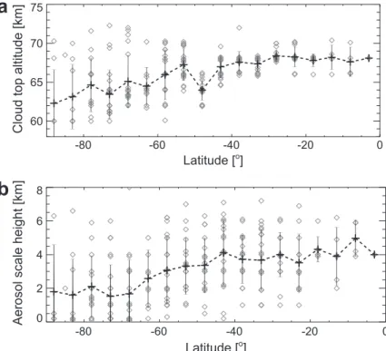
1.1 a: Cloud top altitude along latitude. b: Aerosol scale height along latitude. (Lee et al. (2012)) . . . 4
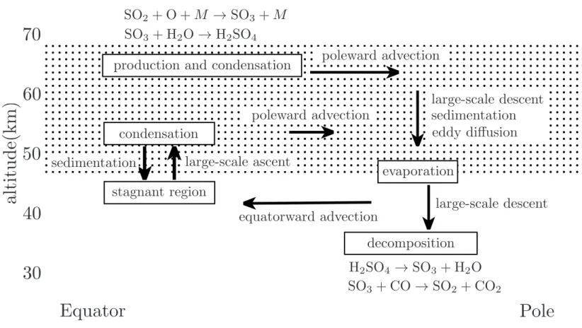
1.2 Schematic view of atmospheric circulation . . . 7
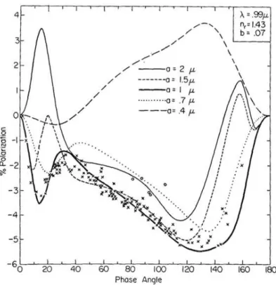
1.3 A comparison between theoretical models (lines) for several effective radius a of cloud particles and observations (points) at λ = 990nm obtained in 1950’s and 1960’s. Since the curves strongly respond to the variations of the parameters, parame- ters of cloud particles can be accurately estimated. . . 8
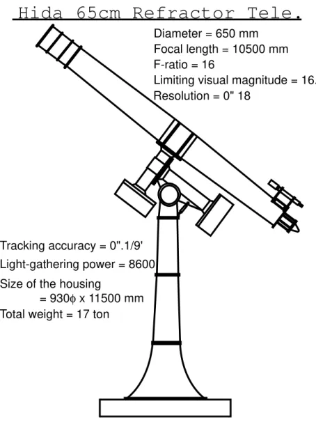
2.1 An illustration of the Hida 65-cm refractor telescope from Web site of the Hida observatory (https://www.kwasan.kyoto- u.ac.jp/general/facilities/65cm/). . . 12
ix
x LIST OF FIGURES 2.2 Upper picture is the exterior view, and lower figure is the
schematics of the optical system of HOPS. The collected light from the telescope is collimated through Zoom Nikkor (Col- limator). The collimated light passes through the half-wave retarder (HWR) and Wollaston prism, and again collected on the surface of the CCD detector by Nikkor (Collector). The symbols “|” and “•” indicate the direction of the optic axis of the calcite, parallel and perpendicular to the plane of paper, respectively. At the same time, the directions of vibration of e-ray and o-ray is perpendicular and parallel to the plane of paper. The optical system is obscured by blackout curtain to avoid stray light from outside. . . 15
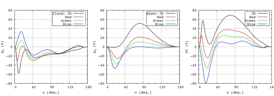
2.3 Single scattering DOPL from cloud and haze particles (left and center), and polarization contrast between them (right). Polarization contrast (P C) is the difference of the single scat- tering degree of polarization between haze and cloud parti- cles. These DOLPs are calculated for reff=1.05µm, veff=0.07, nr =1.43 (for IR), 1.45 (for Red, Green, Blue). The larger the P C is, the more sensitive polarimetric observations get. . . 16
2.4 Phase angle dependence of single scattering polarization p of Rayleigh scattering. α is phase angle. ρn= 0.079 corresponds to CO2 molecules, and ρn = 0 corresponds to the isotropic molecules. . . 18
LIST OF FIGURES xi 2.5 An example of aperture photometry. An aperture region sur-
rounded by a red circle with radius Rap is for measuring the intensity of the object including back ground sky counts. The annulus region enclosed between two green circles with radius Rap and Rap+ ∆Rap is for measuring back ground sky counts. 21 2.6 Aperture and annulus dependence of the polarization degrees.
Points for Ran = 30 and 50 pixels are shifted by ±1 pixels for easiness to distinguish different aperture each other. . . 22 2.7 Vertical cloud structure model. The vertical cloud structure
model is considered after Kawabata et al. (1980). Molecules are neglected in the analysis of IR data. . . 25 2.8 The model of the relation between atmospheric pressure and
the altitude from the ground. There are 5 models according to the difference of the latitude. In this study, we used 0◦− 30◦ data for low to middle latitude region, and 75◦ data for polar regions. . . 26 2.9 Calculated optical thickness. The optical thickness of the gas
layer for IR wavelength is about 5% to that for Blue wave- length. Actually this is small enough to be neglected by the altitude of the cloud top around 68km. . . 27 2.10 Latitudinal distribution of upper haze. Latitudinal distribu-
tion of upper haze is linear slope at the boundary latitude ϕn
and ϕs, and constant between them. ∆ϕn and ∆ϕs are the width of the slope. . . 29 2.11 Differences of polarization maps by latitudinal distribution of
upper hazes. (A) ∆ϕ = 0◦, (B) ∆ϕ = 20◦, (C) ∆ϕ = 50◦. ϕ = 40◦ for (A), (B), (C) . . . 30
xii LIST OF FIGURES 2.12 Latitudinal distribution of each layer top. zc,Eq is the cloud
top altitude for equatorial region, zc,N P zc,SP are the cloud top altitude for North and South pole, respectively. Between latitude ϕn(ϕs) and ϕn+∆ϕn(ϕs+∆ϕs), the cloud top altitude decreases from zc,Eq to zc,N P(zc,SP) linearly. . . 31
2.13 A schematic illustration of a planetary disk observed at phase angle α with apparent radius R. An observer is assumed to be located at long distance which can be regarded as infinity. The origin is taken at the center of disk. The point S on the x-axis corresponding to the intensity equator is sub-solar point. The terminator is located at x = −R cos α on the intensity equator. 33
2.14 A comparison of Gaussian function and modified Lorentzian distribution functions with several parameters. “G” and “L” in the legend indicate Gaussian function and modified Lorentzian distribution function, respectively. Compared with Gaussian function, modified Lorentzian distribution functions are sharper. The sharpness can be varied by a. . . 35
2.15 A comparison of best fit functions. The red points are the intensity of the standard star HD154445, measured from its center of gravity. The blue and green curves are the best fit for modified Lorentzian distribution and Gaussian functions, respectively. Modified Lorentzian distribution function can reproduce well the shape of the peak and tail than Gaussian function. . . 36
LIST OF FIGURES xiii 2.16 Comparisons of minimum standard deviations for Gaussian
and modified Lorentzian distribution function. The minimum values of standard deviations are always smaller for modi- fied Lorentzian distribution function than Gaussian function, which indicate the better reproducibility of the modified Lorentzian distribution function. . . 37 2.17 The difference between Gaussian function and modified Lorentzian
distribution function as PSF. The upper images are the ob- served subtracted observed images blurred model images. The left is the result of modified Lorentzian distribution function with a = 1.5, γ = 3, the right is the result of Gaussian function with σ = 4.2. The lower plots are the intensities at the cross section on the intensity equators indicated with green lines in upper images. . . 39 2.18 Temporal variations of γ and a. The values of γ a are obtained
for images taken at the position angles of half wave retarder plate ϕ = 0◦, 22.5◦, 45◦, and 67.5◦. “Average” labels in the rightmost tics are the values for averaged images, not averages of the set of γ and a. . . 40 2.19 Sensitivity tests for cloud parameters for cloud-only model.
Figure (A) is for effective radius reff, (B) is for effective vari- ance veff, and (C) is for refractive index of the particles. . . 46 2.20 Sensitivity tests for haze parameters. (A), (B), and (C) are
the same with figure 2.19, but for haze particles. . . 47 2.21 Single scattering polarizations for reff=0.20, 0.25, and 0.30µm.
The polarizations for reff=0.20µm are similar to these of Rayleigh scattering as shown in figure 2.4. . . 48
xiv LIST OF FIGURES 2.22 reff and τh dependence of polarizations. Although the po-
larizations at certain phase angle only cannot make us to dis- tinguish the difference of τhand reff, but if we observe polar- izations for wide range of phase angles, we can do it. In that case, the data can include the temporal variations of them. . . 49
2.23 Histograms of the residuals of polarizations for uncertainties of the sky counts. The width of bins is one-tenth of the maximum of residuals. . . 50
3.1 Comparisons of observed DOLP with previous studies. “1960’s” and “PVO early” indicated by black circles are taken from Kawabata et al. (1980), both are disk-averaged DOLP. “PVO early” data are affected by positive polarizations from hazes, between phase angle of 45◦ and 160◦. Our data in 202-Aug. also indicate such existence of hazes in the atmosphere. Note that 1960’s data around α ∼ 80◦ might also indicate the exis- tence of hazes. . . 55
3.2 A summary of obtained polarization maps at 930nm wave- length. The numbers on the top left corner are the sequential set number of observations. Cloud particles generate negative polarization at this wavelength, while haze particles generated negative polarizations. The positive polarizations on the polar regions in August 2012 indicate the existence of upper hazes. . 56
LIST OF FIGURES xv 3.3 Compariaons of integrated DOLP and polarization maps of
observations with theoreticals. The contour maps here are the maps including the best fit parameters of ϕn, ϕs, ∆ϕn,
∆ϕs. The colors of squares on the contours indicate the value of ∆P ; Green: ∆P < Pe/4, Black: ∆P < Pe/2, Magenta:
∆P < 3Pe/4, Red: ∆P < Pe. . . 58
3.4 Same as figure 3.2, but for Blue data. Positive polarization can be generated by Rayleigh scattering from molecules in upper atmosphere, which is the indication of the layer top altitude. . 63
4.1 Comparisons of polarization maps of observed and theoreticals at 438nm wavelength. The theoretical maps on the 2 right- most columns are calculated for different zc,N P and zc,SP of 68km and 75km. The cloud top altitudes of equatorial regions are fixed to zc,Eq=75km. The positive polarizations at this wavelength are generated by Rayleigh scattering. . . 67
4.2 The parameters for examinations. Each figure is the latitu- dinal profile of (a)the extinction coefficient at 80km altitude (dots are taken from Wilquet et al. (2012)), (b) the cloud top altitude (dots are taken from Lee et al. (2012)), (c) the aerosol scale height (dots are taken from Lee et al. (2012)). (d) and (e) are calculated optical thickness using the latitudinal profiles of (b) and (c), respectively. . . 71
xvi LIST OF FIGURES 4.3 The simulations of the aerosol scale height dependence of τh and
fh. (a) The vertical profile of the extinction of the cloud and haze. Several lines for haze is the examples for various value of x. (b)(c) The factor dependence of the optical thickness and fraction of haze. (b) is for Bh = 100Bh,o, and (c) is for Bh = 20Bh,o. . . 76 4.4 (A) Inter comparison between optical thickness of upper haze
at λ = 365nm and SO2 abundance during PVO mission period [After Esposito et al. (1988)]. (B) Scatter plot of optical thick- ness of upper haze (τ365) and SO2 abundance. Data points are taken from (A). . . 77 4.5 SO2 abundance observed in PVO and VEx mission period
[Marcq et al. (2013)]. Red circles are estimated value from equation 4.9 with obtained optical thickness of upper haze in this study. . . 78 4.6 Sunspot relative number observed in National Astronomical
Observatory Japan, Mitaka. This image is taken form http: //solarwww.mtk.nao.ac.jp/jp/solarobs.html. The expla- nations about the indexes from A to E are described in the text. . . 78 4.7 Phase angle dependence of the flux of Venus (Satoh et al.
(2015)), which reflects the characteristics of the cloud and haze in the atmosphere. . . 79
Chapter 1
Introduction
Venus is entirely shrouded by thick cloud of concentrated sulfuric acid (H2SO4). Such particles play important roles in the upper atmosphere of Venus by scattering and absorbing the incident sunlight, thereby affecting the tem- perature and the chemistry. Therefore, studying generation and sustention mechanism of the massive cloud system is essential for deep understanding of the chemical process, radiative balance of the atmosphere, and atmospheric dynamics.
1.1 Structure of the Venusian cloud
The aerosol particles in the cloud can be characterized into 3 modes in terms of the size; Mode 1 particles with radius r ∼ 0.2µm, mode 2 particles r ∼ 1 µm, and Mode 3 particles r ∼ 3µm. The cloud is located in altitude from 50 to 70 km. These facts are clarified from several in situ measurements by entry probes [cf. Knollenberg and Hunten (1980)]. This cloud layer can be categorized to cloud layers (Upper, Middle, and Lower cloud layer) and 2 haze layers (Upper, and Lower haze layer) as listed in table 1.1 [Esposito et al.
1
2 CHAPTER 1. INTRODUCTION (1983)]. Since half of the absorption of incident sunlight in the atmosphere occurs at altitude around 60km [Tomasko et al. (1980)], the existence of the cloud is important in terms of energy deposition.
1.1.STRUCTUREOFTHEVENUSIANCLOUD3 Table 1.1: Vertical structure of Venusian cloud [Esposito et al. (1983)]. Numbers in parenthesis are modes of particles.
Region Altitude Temperature Optical Depth Average Number Mean Diameter Proposed
(km) (K) τ at 630nm Density (N cm−3) (µm) Composition
Upper haze 70-90 225-190 0.2-1.0 500 0.4 H2SO4+
contaminants
Upper cloud 56.5-70 286-225 6.0-8.0 1500(1) Bimodal H2SO4+
50(2) 0.4&2.0 contaminants
Middle cloud 50.5-56.5 345-286 8.0-10.0 300(1) Trimodal H2SO4+
50(2) 0.3, 2.5, & crystal(?)
10(3) 7.0
Lower cloud 47.5-50.0 367-345 6.0-12.0 1200(1) Trimodal H2SO4+
50(2) 0.4, 2.0, & crystal(?)
50(3) 8.0
Lower haze 31-47.5 482-367 0.1-0.2 2-20 0.2 H2SO4+
contaminants Precloud layers 46 & 378 & 367 0.05 & 0.1 50 & 150 Bimodal H2SO4+
47.5 0.3 & 2.0 contaminants
4 CHAPTER 1. INTRODUCTION The latitudinal dependence of the cloud top have been studied by sev- eral authors . Lee et al. (2012) studied about the latitudinal dependence of the cloud top altitude in terms of remote sensing by analyzing near-infrared spectroscopic data by VIRTIS (Visible and Infrared Thermal Imaging Spec- trometer) and temperature profile by VeRa (Venus Radio Science: Radio sounding experiment), both onboard Venus Express, and showed the latitu- dinal profile of the cloud top altitude and aerosol scale height (Figure 1.1). The cloud top altitude from equatorial to middle latitude (∼50◦) is around
-80 -60 -40 -20 0
Latitude [o] 60
65 70 75
Cloud top altitude [km]
-80 -60 -40 -20 0
Latitude [o] 0
2 4 6 8
Aerosol scale height [km]
a
b
Figure 1.1: a: Cloud top altitude along latitude. b: Aerosol scale height along latitude. (Lee et al. (2012))
68km level, but decreases with latitude to 62km level. Although the cloud top altitudes are different for wavelength, such variations were observed in
1.2. MODEL OF CHEMISTRY OF THE CLOUD AND ITS ADVECTION5 other wavelength regions (cf. Zasova et al. (2007), Ignatiev et al. (2009)). The similar variation was observed for aerosol scale height, which shows simi- lar decrease with latitude, from ∼4km in equatorial to middle latitude region to 2km in polar region.
These variations in vertical and horizontal structure of the cloud are im- portant in terms of energy balance, because these variations can change the profiles of the atmospheric heating. At the same time, they are also impor- tant for remote sensing since these variation can affect the morphology, thus interpretation of the observations.
1.2 Model of chemistry of the cloud and its
advection
The source of the cloud is thought to be SO2 in the atmosphere. SO2 is oxidized by photochemically-produced O atoms,
SO2+ O + M → SO3+ M, (1.1)
and SO3 reacts with H2O, and is transformed to H2SO4,
SO3+ H2O → H2SO4. (1.2) These reactions, thus the production of cloud particles, mainly occur at
∼62 km altitude within a thin layer of few kilometers [Yung and Demore (1982), Krasnopolskii and Parshev (1983)]. While there is few observational proof about meridional circulation in Venusian atmosphere, we show here a model that includes advection of chemical materials proposed by Imamura and Hashimoto (1998). Generated cloud particles are transported by pole- ward advection, which is confirmed by cloud tracking study by Rossow et al.
6 CHAPTER 1. INTRODUCTION (1990) and is regarded as upper part of the meridional circulation, to polar regions. Around the poles, sedimentation occurs and cloud particles evapo- rate below the cloud bottom.
1.2.MODELOFCHEMISTRYOFTHECLOUDANDITSADVECTION7 ]
30
40
50
60
70
al ti tu d e( k m )
Equator Pole
large-scale descent equatorward advection
SO2 + O + M → SO3 + M SO3+ H2O → H2SO4
H2SO4 →SO3 + H2O SO3+ CO → SO2+ CO2
production and condensation poleward advection
large-scale descent sedimentation eddy diffusion
evaporation
decomposition stagnant region
condensation
sedimentation large-scale ascent
poleward advection
Figure 1.2: Schematic view of atmospheric circulation
8 CHAPTER 1. INTRODUCTION
1.3 Polarimetry of Venus
Polarimetry is a powerful tool to investigate cloud particle size and refractive index, and cloud vertical structure. The first systematic polarimetric analy- sis was carried out by Hansen and Hovenier (1974), who analyzed 1950’s and 1960’s ground-based data of disk-averaged polarization (Figure 1.3). The ]
Figure 1.3: A comparison between theoretical models (lines) for several ef- fective radius a of cloud particles and observations (points) at λ = 990nm obtained in 1950’s and 1960’s. Since the curves strongly respond to the vari- ations of the parameters, parameters of cloud particles can be accurately estimated.
cloud model used in the radiative transfer calculations was simple semi-
1.3. POLARIMETRY OF VENUS 9 infinite cloud composed of micron-sized cloud particles. The refractive index of the cloud particle was nr= 1.43 at λ=990nm, and the effective radius and variance in a particle size distribution were reff=1.05µm and veff=0.07, re- spectively. The wavelength dependence of the refractive index indicated 75% H2SO4 solution as composition of cloud particles. Kawabata et al. (1980) an- alyzed polarimetric data taken by Orbiter Cloud Photo-polarimeter (OCPP) onboard Pioneer Venus Orbiter (PVO) in early period of the mission. They found that there was a large amount of submicron-sized particles, “hazes”, distributed mixed in and above the cloud layer. The properties of these par- ticles are reff=0.23µm, veff=0.18 and nr = 1.45 at λ =935nm, which has no conflicts with sulfuric acid. Additionally, the spatial distribution of the up- per haze was not uniform. While the optical thickness of upper haze on the equatorial region was 0.02, that on both polar regions was 0.3 at λ=935nm. Temporal variations of such parameters were also reported by several authors (e.g. Sato et al. (1996), Knibbe et al. (1998), Braak et al. (2002)). Sato et al. (1996) reported that the optical thickness of upper hazes on Northern polar region decreased from 0.3 to 0.05 at λ=935nm during the first 2820 days of PVO mission period, and the properties of hazes (reff=0.25µm, veff=0.17 and nr = 1.43 at λ =935nm) were quite stable in its mission period. Recently, European Venus exploration spacecraft, Venus Express (VEx), investigated physical and chemical properties of aerosols in the upper atmosphere from various aspects. As a recent polarimetric study, the preliminary results of Rossi et al. (2015) with polarimetric observations from SPICAV instrument showed that though there were time variations in the optical thickness of the upper hazes, the upper limit of them in 2010 is 0.17 at λ = 1.101µm, which is comparable with the value of Kawabata et al. (1980).
The temporal variation is pointed out to be related to the amount of
10 CHAPTER 1. INTRODUCTION SO2 in the atmosphere since they have positive correlation in long-term variation (Esposito et al. (1988)). However, there is no study about the correlations after PVO mission while Marcq et al. (2013) reported that the amount of SO2 had decreased in the mission period of Venus Express from 2007.
1.4 The objectives of this study
In order to achieve the knowledge of generation and sustention mechanism of Venusian upper haze, we set goals of this study as (1) Track the temporal variations of the haze by carrying out ground-based observations, (2) Inter- pret the obtained physical parameters by simulations with known physical properties, and (3) Propose the possible factor for the temporal variations of haze.
Chapter 2
Methodology
2.1 Observation
2.1.1 Imaging-polarimeter “HOPS” and Hida 65-cm
refractor telescope
Polarimetric observations were performed with an imaging-polarimeter “HOPS” (an acronym of Hida Optical Polarimetry System) attached to the 65-cm refracting telescope (figure 2.1) at the Hida Observatory of the Kyoto Uni- versity (Takayama, Gifu, Japan). This telescope (the focal length is 10.5 m) is favored for polarimetry of planets for 3 reasons: 1) the atmospheric condition is relatively stable at the site; 2) the telescope’s long optical tube is supported by a robust structure; and 3) the optics is perfectly symmetry with no reflecting mirror or obstacle throughout the ray path.
A set of chromatic-aberration correction lenses is inserted between the 65-cm objective lens and HOPS. There are 3 positions: lens B is for short wavelengths (400–500 nm); lens R is for 600 nm and longer wavelengths; and blank for wavelengths between 500 and 600 nm.
11
12 CHAPTER 2. METHODOLOGY
Diameter = 650 mm Focal length = 10500 mm F-ratio = 16
Resolution = 0" 18
Light-gathering power = 8600
Limiting visual magnitude = 16.2
Size of the housing
= 930φ x 11500 mm Total weight = 17 ton Tracking accuracy = 0".1/9'
Hida 65cm Refractor Tele.
Figure 2.1: An illustration of the Hida 65-cm refractor telescope from Web site of the Hida observatory (https://www.kwasan.kyoto- u.ac.jp/general/facilities/65cm/).
HOPS is a 2-beam type imaging polarimetry instrument (Satoh et al. (2001)), which consists of a super-achromatic half-wave retarder plate (on a rotating mount) and a single Wollaston prism. The optical system of the instrument is shown in figure 2.2.
2.1. OBSERVATION 13
Table 2.1: Properties of CCD
Pixel format 1024 pixel × 1024 pixel Length of the side of a pixel 24µm
Length of the side of the CCD detector 24.6 mm × 24.6 mm
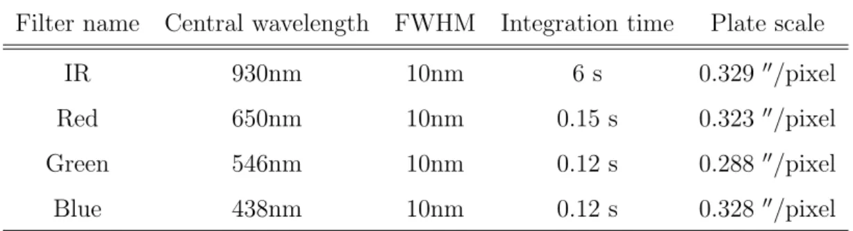
Table 2.2: Properties of filters. FWHM is full width at half maximum.
Filter name Central wavelength FWHM Integration time Plate scale
IR 930nm 10nm 6 s 0.329′′/pixel
Red 650nm 10nm 0.15 s 0.323′′/pixel
Green 546nm 10nm 0.12 s 0.288′′/pixel
Blue 438nm 10nm 0.12 s 0.328′′/pixel
The detector is a Peltier-cooled CCD (SBIG, STL-1001E), of which prop- erties are listed in table 2.1. HOPS has a set of 4 narrow-band filters, λ=438nm (Blue), 546nm (Green), 650nm (Red), and 930nm (IR). The prop- erties are listed in table 2.2.
2.1.2 Description of polarization state
State of polarization of observed light can be described by a set of Stokes parameters, I, Q, and U . Another Stokes parameter, V , which describes cir- cular polarization, is not considered here as reflected sunlight from Venus is known to have very little circular polarization (Kawata (1978)). Two param- eters, Q, and U , are interchangeable as the coordinate system is rotated, and U becomes almost zero when the intensity equatorial plane (a plane which
14 CHAPTER 2. METHODOLOGY includes the sun, center of Venus, and the observer) is taken as a reference plane from which position angle of (Q, U ) vector is measured. Therefore, we hereafter call Q/I “degree of linear polarization” (DOLP). In this case, positive Q corresponds to the polarization with the vibration perpendicular to the reference plane.
2.1.3 Phase angle and observing wavelength
To extract physical information of the haze layer from the data most effi- ciently, we have carried out observations and chosen the data that satisfy following two conditions: the phase angle α is ∼ 80◦, and the data were taken with the IR filter. The reasons are:
1. Contrast of polarizations between haze and cloud is maximum in IR, 2. apparent diameter of Venus is sufficient to overcome the seeing effect,
and
3. elongation to the sun is large, thus stray light from the sun is minimized. Since observed DOLPs are the results of multiple light scattering in the atmosphere, they should be smaller than those of single scattering. But the characteristics, such as the sign of DOLP and the phase angle α making DOLP 0%, is not significantly different from that of single scattering, so we can estimate the combinations of α and λ most sensitive to the amount of hazes, based on theoretical calculations of single scattering polarizations. Figure 2.3 shows the phase angle and wavelength dependence of ph and pc, theoretical DOLP of single scattering generated by haze and cloud particles, and polarization contrast (P C) defined as P C = ph− pc.
2.1. OBSERVATION 15
Telescope
Zoom Nikkor 80-200mm
Wollaston Prism
Nikkor 135mm Super Achromatic
Half-Wave Plate
CCD Camera
Wollaston
HWR
Collimator Collector
Filter
CCD
o-ray
e-ray
Figure 2.2: Upper picture is the exterior view, and lower figure is the schemat- ics of the optical system of HOPS. The collected light from the telescope is collimated through Zoom Nikkor (Collimator). The collimated light passes through the half-wave retarder (HWR) and Wollaston prism, and again col- lected on the surface of the CCD detector by Nikkor (Collector). The symbols
“|” and “•” indicate the direction of the optic axis of the calcite, parallel and perpendicular to the plane of paper, respectively. At the same time, the directions of vibration of e-ray and o-ray is perpendicular and parallel to the plane of paper. The optical system is obscured by blackout curtain to avoid stray light from outside.
16CHAPTER2.METHODOLOGY
-80 -60 -40 -20 0 20 40 60 80
0 45 90 135 180
PC [%]
α [deg.] IR Red Green Blue
-80 -60 -40 -20 0 20 40 60 80
0 45 90 135 180
pc [%]
α [deg.] Cloud: IR
Red Green Blue
-80 -60 -40 -20 0 20 40 60 80
0 45 90 135 180
ph [%]
α [deg.] Haze: IR
Red Green Blue
Figure 2.3: Single scattering DOPL from cloud and haze particles (left and center), and polarization contrast between them (right). Polarization contrast (P C) is the difference of the single scattering degree of polarization between haze and cloud particles. These DOLPs are calculated for reff=1.05µm, veff=0.07, nr =1.43 (for IR), 1.45 (for Red, Green, Blue). The larger the P C is, the more sensitive polarimetric observations get.
2.2. DATA REDUCTION 17 The sensitivity to the amount of haze is higher for large positive or neg- ative P C; (1) α ∼ 20◦, λ=438nm and (2) α ∼ 80◦, λ=930nm. Because the apparent diameter of Venus at α ∼ 20◦ is smaller than 16′′ as mentioned in the above, the polarization map at ∼ 20◦ phase angle will not be used while α ∼ 80◦ may be used if the seeing was good. In addition, the data at small or large α (near 0◦ or 180◦) may be affected by sunlight as elongation to the sun is small. We therefore selected the data satisfying the condition (2) as the most useful combination of phase angle and observing wavelength. Details of observational condition are listed in the Result section. Additionally, cloud top altitude can be estimated from Blue data by considering Rayleigh scat- tering. The polarization degrees of single scattering by Rayleigh scattering can be described as
p(α) = sin
2α
1 + cos2α + 2ρn/(1 − ρn), (2.1) where α is phase angle and ρn is the depolarization factor, which depends on the kind of molecule (The shape of this function is shown in figure 2.4). This function gets maximum at α = 90◦and pc is close to 0% in this wavelength at this phase angle, it is convenient to perform this analysis with this condition.
2.2 Data reduction
2.2.1 Dark current and flat field correction
Although linearity of CCD device is superb, it requires two major corrections. One is the dark noise, which is caused by thermally-generated electrons in Si substrate. A Peltier cooler keeps the CCD at a stable low temperature, re- ducing the noise and maintaining it at a constant level (electrons per pixel per second). Another is non-uniformity of sensitivity. Since this non-uniformity
18 CHAPTER 2. METHODOLOGY
0 10 20 30 40 50 60 70 80 90 100
0 30 60 90 120 150 180
p [%]
α [deg.]
ρn=0.079 ρn=0.000
Figure 2.4: Phase angle dependence of single scattering polarization p of Rayleigh scattering. α is phase angle. ρn = 0.079 corresponds to CO2
molecules, and ρn= 0 corresponds to the isotropic molecules.
is permanent feature and is fixed to pixels, this can be removed by dividing an object image by a flat-field image. A flat-field can be obtained by imaging a uniformly-illuminated object. In this study, we took clear sky by pointing the telescope to the zenith.
Because a flat-field image F also includes dark current D, one raw image R can be processed to obtain a corrected image C as follows:
C = (R − D)
(F − D)/N, (2.2)
where N is a normalization factor of F − D image.
2.2. DATA REDUCTION 19
2.2.2 Derivation of Degree of Linear Polarization (DOLP)
A 2-beam type polarimeter measures intensities of light in 2 beams (called ordinary and extraordinary rays) oscillating in planes perpendicular to each other. By repeating measurements for 4 position angles (0◦, 22.5◦, 45◦, and 67.5◦) of a half-wave retarder plate, this type of instrument allows polarime- try of high accuracy (Tinbergen (1996)). The degrees of linear polarization are calculated by following equations (Tinbergen (1996));
Q
I =
1 − a1 1 + a1
(2.3)
with a1 =
√ Ie(0◦) Io(0◦)
/ Ie(45◦) Io(45◦) U
I =
1 − a2
1 + a2 (2.4)
with a2 =
√
Ie(22.5◦) Io(22.5◦)
/ Ie(67.5◦) Io(67.5◦)
where Io(ϕ) and Ie(ϕ) are intensities of the light separated for ordinary and extraordinary ray, respectively; ϕ is the position angle of half-wave plate installed in front of a Wollaston prism.
2.2.3 Calibration of instrumental polarizations
Although the optics of HOPS and the 65-cm telescope is symmetry, there still remain instrumental polarizations of small amplitudes. We have carefully examined flat-field images (acquired in the daytime of observing run) and obtained experimental values of such polarization as a function of position in the field of view. In the data analysis, the Venus data are corrected for by subtracting the instrumental polarization.
20 CHAPTER 2. METHODOLOGY
2.2.4 Consideration of atmospheric seeing
One major and unavoidable problem of ground-based observation is variable atmospheric seeing, which blurs the image and alters the intensity distribu- tion over the planetary disk with different degrees from one image to another. This obviously could cause errors in polarimetry as the seeing changes while we acquire a set of images at 4 position angles of the half-wave retarder plate in HOPS. In order to reduce the effect of atmospheric seeing, we perform both aperture photometry and analysis of 2-dimensional polarization maps. The aperture photometry is a way to avoid the effect of atmospheric seeing, in sacrifice of spatial information, by measuring polarization of integrated light from the object. On the other hand, to better utilize information of 2-dimensional polarization maps from HOPS, the data are filtered by the
“measured” seeing size. If the seeing size is larger than 14 in γ described in equation (2.20), corresponding 2-dimensional map is discarded.
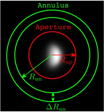
Figure 2.5 illustrates an example of aperture photometry of Venus. An aperture is a circular region of which radius Rap is large enough to integrate super-majority of light from the object. An annulus, used to determine the background level, is a region between two circles with radius Ran and Ran+ ∆Ran large enough to avoid the tail of blurred light of the object.
Intensities of the object Iobj, Venus in this study, are calculated by the following equation;
Iobj =
Nap
∑
i=1
Ii− NapIbg (2.5)
Ibg =
Nan
∑
j=1
Ij/Nan (2.6)
where Nap and Nan are the number of pixels in the aperture and the annulus, respectively.
2.2. DATA REDUCTION 21
Annulus
Aperture
∆R
anR
anR
apFigure 2.5: An example of aperture photometry. An aperture region sur- rounded by a red circle with radius Rap is for measuring the intensity of the object including back ground sky counts. The annulus region enclosed between two green circles with radius Rap and Rap+ ∆Rap is for measuring back ground sky counts.
In order to determine the size of aperture and annulus, we performed test calculations for several combinations of these parameters. Figure 2.6 shows an example of the aperture and annulus dependence of DOLP for April 2014 set01 data with angular radius of Venus Rv = 27.5 pixels. The data points are DOLP for Rap = 30, 40, and 50 pixels, and Rap from corresponding value of Rap. ∆Rap is fixed to 5 pixels. In case of Rap = 30 pixels, the DOLP is negatively overestimated because the aperture is slightly small to integrate all the light from the object blurred by the atmospheric seeing. On the
22 CHAPTER 2. METHODOLOGY
-3.6 -3.4 -3.2 -3 -2.8 -2.6
30 35 40 45 50 55 60 65 70 75 80
DOLP [%]
Ran [pixel]
2014-04 set01: Rv = 27.5 pix Rap = 30 pix
40 pix 50 pix
Figure 2.6: Aperture and annulus dependence of the polarization degrees. Points for Ran = 30 and 50 pixels are shifted by ±1 pixels for easiness to distinguish different aperture each other.
other hand, DOLP with Rap=40, and 50 pixels for over Ran = 55 pixels is stable, which means that the tail of the blurred light converges around Rap
= 40pixels. Since enlarging the value of Rap too much may carry a risk of involving unexpected errors, we determined the size of aperture and annulus as Rap = 1.5Rv, and Ran = Rap + 15 pixels, respectively.
2.3 Model calculation
Numerical computation of the polarized light from Venus is done in 3 steps: 1. A single scattering matrix (a transformation matrix between Stokes
2.3. MODEL CALCULATION 23 parameters of the incident light and the scattered light) based on Mie theory is obtained with a published computational code by Mishchenko et al. (2002).
2. Using the resultant single scattering matrix, we carry out radiative transfer calculations with the effect of multiple light scattering is taken into account for. Computational code for this has been domestically developed by referring to de Haan et al. (1987) and Hovenier et al. (2004).
3. A model polarization map is produced by pixel-by-pixel computations of I and Q for scattering geometries of individual pixels. Obtained map is then blurred with an appropriate point-spread function (PSF) discussed in the followings.
2.3.1 Cloud structure model
We define cloud, haze, and molecular particles as follows; Cloud reff=1.05µm, veff=0.07, nr, and ϖ0,c
Haze reff=0.25µm, veff=0.17, nr, and ϖ0,h
Molecule CO2 molecule, with depolarization factor ρn= 0.079, and ϖ0,m
where nr is real part of the refractive index, and ϖ0 is the single scattering albedo. nr is fixed to nr = 1.43 and 1.45 for IR and Blue, respectively. reff, veff, and nr are taken from previous studies (cf. Sato et al. (1996), Knibbe et al. (1998),Braak et al. (2002)). These values were quite stable through 8 years from the starting date of PVO mission[Sato et al. (1996)]. The size distribution of the particles is a modified gamma distribution function
24 CHAPTER 2. METHODOLOGY described as
N (r) = Cr−3+(1/veff)exp (
−r r
effveff
)
, (2.7)
where C is a constant for normalization. Single scattering albedos of the cloud particles are calculated to force spherical albedo to match that of ob- served with the similarity relation
ϖ0 = 1 − (1 − ϖ0iso)(1 − ⟨cos θ⟩), (2.8) where ϖ0iso is the single scattering albedo of the isotropic scattering with τ = ∞, and ⟨cos θ⟩ is the asymmetry parameter of the phase matrix of the as- sumed particles [Hansen and Hovenier (1974)]. From Chamberlain and Smith (1970) and Mie scattering calculation, we have ϖiso0 =0.99741 and 0.97940, and ⟨cos θ⟩=0.702 and 0.75 for λ =930nm and 438nm, respectively. Then single scattering albedo of cloud particles are calculated to be ϖ0,c =0.99923 and 0.99485 for λ =930nm and 438nm, respectively. Single scattering albedo of haze and molecules, ϖ0,h and ϖ0,m, were fixed to 1 because contributions of the hazes to the spherical albedo are small compared with that of cloud particles, and absorption by CO2 molecule is small in visible to near infrared (λ <1000nm) range [Moroz (1983)].
Rayleigh scattering from molecules is not included in the analysis at λ =930nm because the contribution from gas molecules is sufficiently small at this wavelength; The scattering cross section of Rayleigh scattering is pro- portional to λ−4 and can produce few contribution to observed polarizations at longer wavelength (the scattering cross section at 930nm is less than 5% of that at 438nm). However, the contribution of the Rayleigh scattering at λ =438nm is significant, Rayleigh scattering is considered in model calcula- tions at this wavelength for estimation of cloud top altitude.
ρnis the depolarization factor, which characterizes the polarization degree of Rayleigh scattering. Though the polarization degree from an isotropic
2.3. MODEL CALCULATION 25
Cloud particles Haze particles Molecules
Cloud Layer
Haze Layer
Gas Layer
τ
h+ τ
R′τ
c+ τ
h′+ τ
R′′= 256
τ
RFigure 2.7: Vertical cloud structure model. The vertical cloud structure model is considered after Kawabata et al. (1980). Molecules are neglected in the analysis of IR data.
molecule at phase angle of 90◦ is 100%, that from an unisotropic molecule is lower than 100%. Therefore, this value depends on the kind of molecule. For example, ρn= 0.020 for N2, 0.058 for O2, 0.028 for dry air, and 0.079 for CO2. Since the atmosphere of Venus is composed of 96.5% CO2 [Hovenier et al. (2004)], we used ρn = 0.079.
Figure 2.7 shows the vertical cloud structure model used in radiative transfer calculations. This model is composed of three layers: main “cloud layer”, middle “haze layer”, and upper “gas layer”. Since the multiple scat- tering of the lights in the atmosphere reduce the features of the polarizations and make them essentially unpolarized, the feature of linear polarizations are mostly determined by the first several orders of the scattering, down to the layers of the optical thickness unity. So we don’t have to model the details of the deep cloud layers which were studied with entry probe measurements.
26 CHAPTER 2. METHODOLOGY
60 65 70 75 80 85 90 95 100
0.01 0.1 1 10 100 1000
z [km]
p [mbar]
Lat.: 0 - 30 deg. 45 deg. 60 deg. 75 deg. 85 deg.
Figure 2.8: The model of the relation between atmospheric pressure and the altitude from the ground. There are 5 models according to the difference of the latitude. In this study, we used 0◦ − 30◦ data for low to middle latitude region, and 75◦ data for polar regions.
The gas layer is composed only molecules with optical thickness τR. τR
is calculated from the equation
τR = 1 + 0.013λ
−2
6.17 × 10⁴λ4p(z), (2.9)
where λ is the wavelength in µm, and p(z) is the pressure in mbar at altitude z (Hansen and Travis (1974)). The relations between pressure p and altitude z are taken form Seiff (1983) as shown in figure 2.8. Calculated optical thickness of gas layer is shown in figure 2.9 for both Blue and IR wavelength. This indicates that the optical thickness of the gas layer for IR wavelength is 5% of Blue wavelength and small enough to neglect at the IR wavelength.
2.3. MODEL CALCULATION 27
60 65 70 75 80 85 90 95 100
0 0.02 0.04 0.06 0.08 0.1
z [km]
τR
IR Blue
Figure 2.9: Calculated optical thickness. The optical thickness of the gas layer for IR wavelength is about 5% to that for Blue wavelength. Actually this is small enough to be neglected by the altitude of the cloud top around 68km.
The haze layer is composed of haze particles and molecules with optical thickness τhand τR′, respectively. The main cloud layer is a mixture of cloud, haze particles, and molecules with optical thickness τc+ τh′+ τR′′ = 256 (virtu- ally semi-infinite). The haze and cloud particles are mixed with the fraction fh defined by
fh = ksca,h ksca,c+ ksca,h
, (2.10)
where ksca,h and ksca,c are scattering coefficient of haze and cloud particles, respectively. Here we assumed kabs,c = 0 because this factor is smaller by 10−5 to ksca,c. Scattering matrix Z, which represents the properties of single
28 CHAPTER 2. METHODOLOGY scattering in the layer, are calculated as
Z = fhZh+ (1 − fh)Zc, (2.11) where Zh and Zc are scattering matrices of haze and cloud particles, re- spectively. The optical thickness of haze in the cloud layer τh′ also can be calculated as
τh′ = fh
1 − fhτc. (2.12)
τR′′ can be calculated as
τR′′ = fR
1 − fRτp, (2.13)
where fRis the Rayleigh fraction, and τp = τc+τh′. The definition of Rayleigh fraction is
fR= ksca,R
ksca,p+ ksca,R, (2.14)
where ksca,R is the scattering coefficient of Rayleigh scattering, and ksca,p = ksca,c + ksca,h. The values of fR were 0.043, 0.025, and 0.033 at λ =365nm in Hansen and Hovenier (1974), Kawabata et al. (1980), and Braak et al. (2002), respectively. Assuming τc = 30 at this wavelength, which is consistent with in situ measurements [Esposito et al. (1983), Ragent et al. (1985)], τR′′ calculated from these values lead the altitude of the bottom of the cloud layer around 50km. Taking this into account, we fixed fR= 0.015 at 438nm, which corresponds to fR = 0.03 at 365nm.
2.3.2 Latitudinal profile of upper haze and cloud top
altitude
Spatial variations in 930-nm polarization maps primarily come from the lat- itudinal distribution of haze. We assume a simple latitudinal distribution model as shown in figure 2.10. Hereafter we call the region of latitude be-
2.3. MODEL CALCULATION 29
τ
h,Nτ
h,Sτ
hNorthern Latitude Southern
Latitude 90◦S 90◦N
τ
h,Eqφ
n∆φ
n∆φ
sφ
sFigure 2.10: Latitudinal distribution of upper haze. Latitudinal distribution of upper haze is linear slope at the boundary latitude ϕnand ϕs, and constant between them. ∆ϕn and ∆ϕs are the width of the slope.
tween ϕn and −ϕs “Equatorial region”, and other polar side regions “North- ern polar region” and “Southern polar region”. From latitude of ϕn (−ϕs) to ϕn+ ∆ϕn (−ϕs− ∆ϕs), we call this “transition region”, optical thickness of upper haze is assumed to linearly increase to τh,N and τh,S. Figure 2.11 illustrates the differences of patterns for different width (∆ϕ) of transition region.
Spatial variations in 438-nm polarization maps come from the altitude of each layer’s top. It is known that the cloud top altitude decreases with lati- tude from around 50◦ to the poles. In order to simulate this fact, we assumed simple model similar to the latitudinal distribution of the optical thickness of the haze layer as shown in figure 2.12. In this model, the boundary lat- itude, at which the cloud tops start lowering, ϕn and ϕs, and the width of the transition ∆ϕn and ∆ϕs are the same with those in figure 2.10.
In the analysis of IR data, as above mentioned, we assumed that the effect of Rayleigh scattering can be neglected, thus, τR = τR′ = τR′′ = 0. We firstly determine fh and τh,Eq on equatorial region by analyzing the regions
30 CHAPTER 2. METHODOLOGY
±0%
-5% +5%
DOLP
(A) (B) (C)
Figure 2.11: Differences of polarization maps by latitudinal distribution of upper hazes. (A) ∆ϕ = 0◦, (B) ∆ϕ = 20◦, (C) ∆ϕ = 50◦. ϕ = 40◦ for (A), (B), (C)
near intensity equator (between −15◦and +15◦) because such regions appear to be free from upper haze. Secondly, we adopt deduced fh to both polar regions. Although fh in the polar regions may not be the same as that of the equator, this treatment may be practical. The reason being that contributions from haze particles mixed in the cloud may well be masked by stronger polarizations of the upper haze if it is optically thick. If the upper hazes on polar regions are thin, hence the polarizations is not dominated by upper hazes, then we may simply re-adjust the value of fh after comparing polarization maps.
The computed points are selected to include the best fit parameters in the range by considering the previous studies and test calculations. Maximum fh and τh,Eq were 0.065 and 0.02 in PVO observations [Kawabata et al. (1980)], and maximum τh,N and τh,S were 0.30 during thick-haze period in 8 years from the beginning of the PVO mission [Sato et al. (1996)]. These can be thought to be the limitation of the points in theoretical calculations. Computation points of ϕn, ϕs, ∆ϕn, and ∆ϕs are determined from the test calculations, and are confirmed to be consistent with the boundary latitude of
2.3. MODEL CALCULATION 31
zc,Eq
zc,N P zc,SP
±0◦ z
φn
φs
∆φs ∆φn 90
◦N
90◦S
Northern Southern
Latitude Latitude
Figure 2.12: Latitudinal distribution of each layer top. zc,Eq is the cloud top altitude for equatorial region, zc,N P zc,SP are the cloud top altitude for North and South pole, respectively. Between latitude ϕn(ϕs) and ϕn + ∆ϕn(ϕs+
∆ϕs), the cloud top altitude decreases from zc,Eq to zc,N P(zc,SP) linearly.
Table 2.3: Range of calculated parameters for IR model fh τh,Eq τh,N τh,S ϕn [◦] ϕs [◦] ∆ϕn [◦] ∆ϕs [◦]
start 0.000 0.00 0.00 0.00 31 31 10 10
end 0.060 0.03 0.30 0.30 49 49 30 30
step 0.005 0.01 0.01 0.01 3 3 5 5
the bright polar caps seen in UV images and previous polarimetric studies[cf. Lee et al. (2015), Kawabata (1981)]. The calculated points are listed in table 2.3.
32 CHAPTER 2. METHODOLOGY
2.3.3 Theoretical calculations for polarization map and
disk-averaged DOLP
We generated theoretical polarization maps calculating I and Q for corre- sponding pixels in images considering local scattering geometries as
µ ≡ cos θ = √R
2− (x2+ y2)
R , (2.15)
µ0 ≡ cos θ0 = µ cos α +x sin α
R , (2.16)
cos(ϕ − ϕ0) = µµ0− cos α
√(1 − µ2)(1 − µ20)
, (2.17)
sin(ϕ − ϕ0) =
y sin α
R√(1 − µ2)(1 − µ20), (2.18) where x and y are the horizontal and vertical coordinate of a point on the planetary disk, viewed from infinity with apparent radius R in pixel unit; θ0
and ϕ0 are zenith and azimuth angles for incident light; θ and ϕ are those for emergent light, as shown in figure 2.13 [after Kawabata (1981)]. The x-axis is taken to be the intensity equator, and the limb of the planet is assumed to be located on the positive domain of x. Disk-averaged DOLP were calculated by taking summations of I and Q for the whole planetary disk.
2.3.4 Point-spread functions to fit the “observed” po-
larization maps
Generally, we cannot get infinitely sharp image but get to some extent blurred image by observing a point source with an optical instrument, because the light is affected by several factors, such as diffraction in the instrument and atmospheric seeing. Such effects appear also in imaging of an disk object like Venus. How does the image spread can be described by functions called point-spread function (PSF). By convolving ideal images with a PSF, we
2.3. MODEL CALCULATION 33
x
y
O
γ
P (x, y)
S R
R
− R
− R cos α − R sin α
Figure 2.13: A schematic illustration of a planetary disk observed at phase angle α with apparent radius R. An observer is assumed to be located at long distance which can be regarded as infinity. The origin is taken at the center of disk. The point S on the x-axis corresponding to the intensity equator is sub-solar point. The terminator is located at x = −R cos α on the intensity equator.
can reproduce the blurred images. Since patterns of polarization maps are affected by such effects, so knowing appropriate PSF is important in eval- uating theoretical and observational polarization maps. In this subsection, we examine HOPS images and determine PSF. The blurring of images in ground-based observations is dominated by atmospheric seeing rather than instrumental factors, so hereafter we assume the source of the blurriness is due to atmospheric seeing.
Blurring of images is most commonly approximated with a Gaussian func- tion;
f (x; σ) = √ 1
2πσ2 exp (
− x
2
2σ2 )
. (2.19)
σ in this equation is the index of the size of PSF. While a Gaussian PSF well
34 CHAPTER 2. METHODOLOGY describes “time averaged” seeing effects, the short-integrated Venus images
“without time averaging” likely require a different shape of PSF. Therefore, we tested a “modified Lorentzian distribution function” in the following form as well:
f (x; a, γ) = C
(x2+ γ2)a, (2.20)
where γ is the size of PSF, a is the index of sharpness, and C is the constant of normalization. Figure 2.14 compares the differences of the shape among Gaussian function and modified Lorentzian distribution functions with sev- eral parameters.
First of all, we compared these 2 functions by adopting them to polar- ization standard stars, which can be regarded as point source. Figure 2.15 is an example which compares the best-fit functions to the radial profile of the standard star HD154445 (R.A.: 17h05m32s.1, Dec.: −00◦53′32′′, Visual magnitude: 5.62), which shows the modified Lorentzian distribution func- tion makes a good fit, and actually the sum of the squared residuals is 15% smaller for modified Lorentzian distribution function. We tested for other stars and found that the sum of the squared residuals is always smaller in case of modified Lorentzian distribution function than Gaussian function. We can say that Lorentzian distribution function works better as the PSF.
We performed the similar process for Venus images to verify the adequacy of the modified Lorentzian distribution function and obtain appropriate PSF. To avoid possible contamination from the polar hazes, we examined limb profiles only near the intensity equator (±15◦) to determine the PSF (either Gaussian or Lorentzian, and the size of PSF). A synthetic image is generated with a “cloud only” model (described in the below) which is then blurred by a PSF with an assumed seeing size. After subtracting observed images, we evaluated the standard deviations of the residual intensities. Such analysis
![Table 1.1: Vertical structure of Venusian cloud [Esposito et al. (1983)]. Numbers in parenthesis are modes of particles.](https://thumb-ap.123doks.com/thumbv2/123deta/6155388.103349/23.1262.193.1097.206.732/table-vertical-structure-venusian-esposito-numbers-parenthesis-particles.webp)