本文 Thesis 総合研究大学院大学学術情報リポジトリ A1718本文

with kernel methods

Hiroshi Yamashita

DOCTOR OF PHILOSOPHY

Department of Statistical Science

School of Multidisciplinary Sciences

The Graduate University for Advanced Studies

2014

Abstract

Small molecules that have the ability to alter the biological response of a cell or disease state are of significant interest as drug candidates. One approach to the design of such molecules using kernel methods is through a map of molecules to a feature space induced by a kernel, where the predictions of the molecular properties are made in a linear manner. The forward mapping helps guide the synthesis of new molecules. Another more direct approach is to solve the so-called pre-image problem, i.e., to reconstruct a corresponding molecule (aka pre-image) from its feature space representation. The inverse mapping is of central impor- tance for the design of new molecules with desired properties. In this thesis, we address two problems in drug design: (I) the forward problem of predicting molecular properties, where we propose a new graph kernel that induces a feature space amenable to the prediction of molecular properties, and (II) the inverse problem of designing new molecules that possess properties required for drug candidates, where we develop a population-based Monte Carlo method to solve the pre-image problem for the molecules. Our respective contributions to these problems are summarized as:

(I) Forward problem of predicting molecular properties

The measurement of molecular similarity is an essential part of predicting molecular prop- erties. Graph kernels provide good similarity measures between molecules. A conventional graph kernel is based on counting common subgraphs of a specific type in molecular graphs. This approach suffers from two primary limitations: (i) only exact subgraph matching is

considered in the counting operation, and (ii) most of the subgraphs will be less relevant to a given task. In order to address these limitations, we propose a new graph kernel as an ex- tension of the subtree kernel initially proposed by Ramon and Gärtner (2003). The proposed kernel tolerates an inexact match between subgraphs by allowing matching between atoms with similar local environments. In addition, the proposed kernel provides a method to as- sign an importance weight to each subgraph according to the relevance to the task, which is predetermined by a statistical test. These extensions lead to promising improvements in classification and regression tasks for predicting a wide range of pharmaceutical properties from the chemical structure of molecules.

(II) Inverse problem of designing new molecules

The de novo design of new molecules that yield desired properties has the potential to sub- stantially reduce both the time and cost involved in drug development. Recent developments in graph kernels have enabled us to apply well-established machine learning techniques to molecular data which are internally represented as graphs. However, in order to allow for the design that generates new molecules as a result, it is necessary to solve the pre-image problem for molecules. Unlike the traditional method proposed in Bakır et al. (2004), which is formulated as a nonlinear combinatorial optimization problem, we express the pre-image problem as a sampling problem for molecular graphs. Here, we are not only interested in optimal molecules, but also in near-optimal molecules which are often considered to be good candidates for further chemical synthesis. Therefore, we develop a population-based Monte Carlo method for sampling structurally diversified molecules near the pre-images, which possess good drug-likeness. The key to an efficient sampling method is to use the update of a population by evolutionary operators for the structural alteration of molecules. Furthermore, to penalize non-drug-like molecules, we use the knowledge of drug-likeness commonly considered by medicinal chemists. The effectiveness of the proposed method is

iii

illustrated through experiments to find corresponding molecules from given image points in a feature space induced by a graph kernel.

Many thanks go to my thesis supervisor, Ryo Yoshida, and sub-supervisor, Tomoyuki Higuchi, for introducing me to the world of machine learning. Ryo has helped me in innumerable ways. I am also very grateful to the members of the Research and Development Center for Data Assimilation.

It goes without saying that my thesis referees, Yoshihiro Yamanishi, Tomoyuki Higuchi, Yukito Iba, Kenji Fukumizu, and Ryo Yoshida have reviewed this thesis and given me valu- able comments to improve upon its content.

Of course, fruitful research is only possible in a friendly and pleasant working envi- ronment. Takashi Washio and Yukito Iba—thanks for our scientific discussions. Okimasa Okada and Tetsu Isomura—thanks for all our discussions. Though I could easily continue this list of colleagues, I wish to thank Masataka Kuroda and Takanori Ohgaru who work in the chemoinformatics group at Mitsubishi Tanabe Pharma Corporation.

Contents

Contents v

1 Introduction 1

1.1 Background . . . 1

1.1.1 Forward Problem of Predicting Molecular Properties . . . 3

1.1.2 Inverse Problem of Designing New Molecules . . . 6

1.2 Outline of the Thesis . . . 8

2 Kernel Methods for Molecules 10 2.1 Kernel Methods . . . 10

2.2 Representing Chemical Structures . . . 13

2.3 Graph Kernels . . . 15

2.3.1 Convolution Kernels . . . 15

2.3.2 Random Walk Kernels . . . 17

2.3.3 Subtree Kernels . . . 18

2.3.4 Other Graph Kernels . . . 20

3 Atom Environment Kernels for the Forward Problem 22 3.1 Basic Idea . . . 22

3.2 Inexact Match Extension . . . 23

3.3 Importance Weight Extension . . . 25

3.4 Relation to Previous Research . . . 28

3.5 Atom Environment Labels . . . 29

3.5.1 Continuous Labels . . . 29

3.5.2 Discrete Labels . . . 30

3.6 Kernel Computation . . . 31

3.6.1 Recursive Algorithm . . . 31

3.6.2 Complexity . . . 32

3.7 Experiments . . . 32

3.7.1 Experimental Settings . . . 33

3.7.2 Data Sets . . . 36

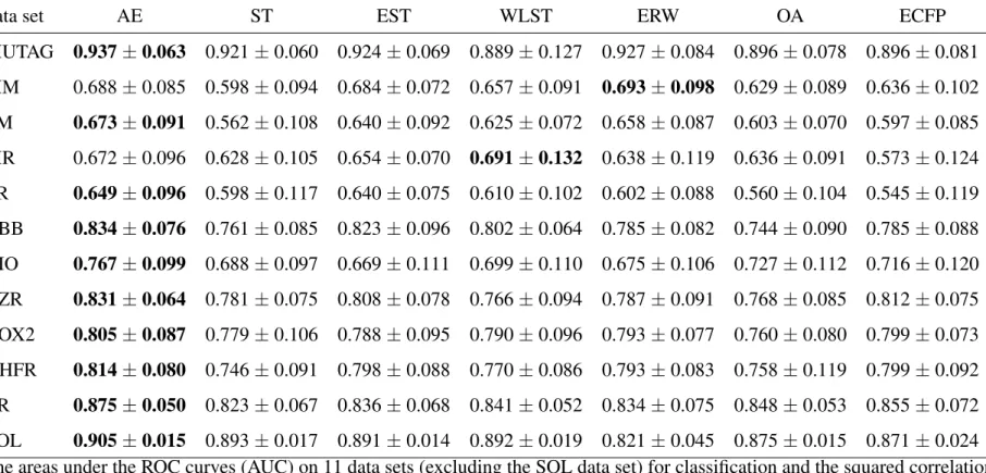
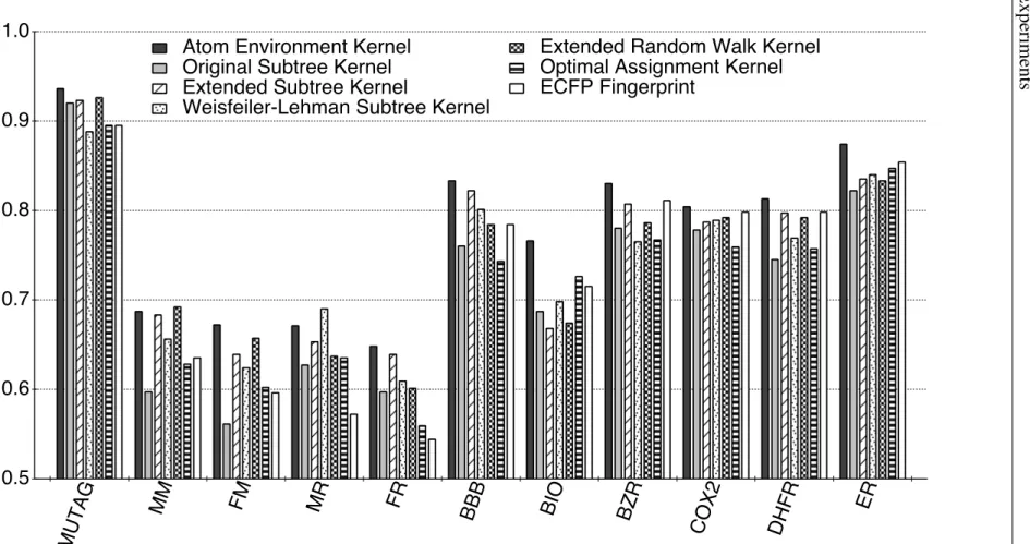
3.7.3 Results and Discussion . . . 37

3.8 Concluding Remarks . . . 47

4 Fragment Assembly Monte Carlo Methods for the Inverse Problem 49 4.1 Basic Idea . . . 49

4.2 Evolutionary Movements in Chemical Space . . . 53

4.3 Preparation of Molecular Fragments . . . 57

4.4 Regularization of Molecules . . . 58

4.5 Experiments . . . 59

4.5.1 Experimental Settings . . . 59

4.5.2 Results and Discussion . . . 61

4.6 Concluding Remarks . . . 65

5 Conclusions 67

Appendix A Derivation of the Recursive Formula 70

List of Figures 73

Contents vii

List of Tables 78

Symbols 82

References 83

List of Publications 92

Introduction

1.1 Background

A primary goal in drug development is to identify new molecules that possess suitable prop- erties required for drug candidates. It is estimated^3–5 that there are in excess of 10⁶⁰ or- ganic molecules below 500 Da of possible interest for drug development. A comprehensive synthesis of molecules is not feasible strategy due to this vast chemical space. Therefore, computer-aided molecular design (CAMD) has the potential to substantially reduce both the time and cost involved in the trial-and-error experiments of drug development. The use of quantitative structure–activity relationships, known as QSARs,^6,7is a promising approach to CAMD. The first step in this approach is to build a forward QSAR model for predicting biological activities or molecular properties from the structural information of a molecule. A forward QSAR can be established using many different model equations (e.g., multi- ple linear regression, partial least squares, support vector regression, etc.). Once a model is built, we next invert the QSAR, i.e., now searching for molecules of interest under the model. This is referred to as the inverse problem.

The most commonly used solution to the inverse problem is virtual screening. In this ap- proach, molecules in a database are evaluated using a forward QSAR to identify molecules

1.1 Background 2

O N

N N

N N O

O N O

S

G

G

φ φ(G)

Input space G Feature space F

forward mapping

inverse mapping

φ

Ψ =

i=1

^α

^φ(G

⁾

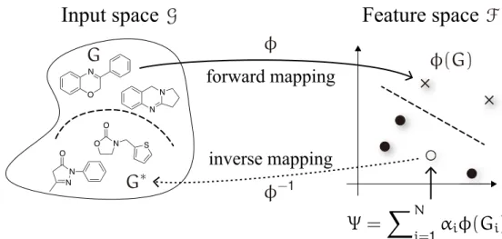
Figure 1.1 Illustration of the pre-image problem in kernel methods. An image pointΨ in the feature space F is mapped back to the input space G.

possessing desired properties. However, virtual screening can only identify molecules present in the database, i.e., it cannot suggest new structural molecules that yield better properties than known molecules. De novo design solves this problem by building molecules from scratch so as to optimize a scoring function. While the scoring is based on a QSAR model, other factors such as drug-likeness and synthetic accessibility can be used as well. Methods for designing new molecules include graphical enumeration^8–10 and stochastic optimiza- tion^11–16 in the context of inverse QSAR. The exhaustive enumeration of chemical struc- tures with given constraints is often computationally demanding. In addition, at present, this approach can generate only treelike (acyclic) molecular graphs. A stochastic approach such as simulated annealing, genetic algorithms, or tabu search solves a nonlinear combinatorial optimization problem for chemical structures, where one may be interested in only optimal solutions of the problem.

Kernel methods^17–20provide a principle framework for solving the forward and inverse problems in CAMD. The recent development of graph kernel functions²¹ has made it pos- sible to apply kernel methods to various machine learning tasks in chemical informatics,²² where graphs are used to describe the chemical structure of the molecules.²³Once a suitable kernel functionk on a set G of molecular graphs is defined, the kernel approach to molecules

works successfully for well-established machine learning methods (e.g., support vector ma- chine, logistic regression, K-means clustering, etc.). The basic idea behind the kernel ap- proach is to implicitly map molecular graphs in the input space G into the high dimensional feature space F via a possible nonlinear map ϕ : G→ F such that for every G, G^′∈ G it holds that k(G, G^′) =⟨ϕ(G), ϕ(G^′)⟩ where ⟨·, ·⟩ denotes the inner product. The forward mapping ϕ is of primary importance in predicting the molecular properties.^24–26 We next invert the forward mappingϕ, i.e., the inverse mapping ϕ⁻¹ from the feature space F back to the input space G. This is known as the pre-image problem. The pre-image problem is of central importance for the design of new molecules with desired properties.^2,27Many graph kernels²¹ for solving the forward problem exist, yet solutions^2,28to the inverse problem are relatively limited due to its ill-posed nature; it is non-convex, nonlinear, and combinatorial. We describe kernel methods to address the forward and inverse problems in detail below.

1.1.1 Forward Problem of Predicting Molecular Properties

The definition of an appropriate similarity function between molecules is of crucial impor- tance for many applications in chemical informatics. Common applications include QSAR model construction to predict biological activities from structural information of molecules. The quantitative structure-activity relationship models rely on the similarity property princi- ple,²⁹which states that structurally similar molecules tend to have similar properties. There- fore, the QSAR model, derived using an appropriate similarity function, will help guide the synthesis of new molecules.

Graphs are often used as a natural mathematical abstraction to describe the chemical structure of molecules.²³ A molecule is translated to a labeled graph (or molecular graph), in which vertices correspond to atoms and edges correspond to covalent bonds between the atoms. The vertices are labeled with element types (e.g., carbon, oxygen, etc.) while the edges are labeled with bond types (e.g., single, double, etc.). Measurement of the similarity

1.1 Background 4

between the molecular graphs requires a method by which to transform any molecular graph G to a feature vector ϕ(G). Classically, molecular graphs are transformed into molecular descriptors,³⁰which can be thought of as numerical representations that are encoded so as to capture the relevant aspects of structural information of molecules. A unique dictionary³⁰ of molecular descriptors lists more than 3, 300 descriptors. Popular choices for them in- clude extended-connectivity fingerprints³¹ (ECFPs). The similarity between the molecular descriptors is then measured by a similarity metric, e.g., the Tanimoto coefficient.³²To date, the molecular descriptors are widely applied due to their computational efficiency. However, such a transformationϕ may cause some loss of structural information of molecules due to the limited dimensional feature space of the molecular descriptors.

Alternatively, molecular graphs can be compared directly in a potentially high or infinite dimensional feature space without the need to perform the explicit transformation,ϕ. This is possible when using a positive definite kernel^19,20k on a set G of molecular graphs. The symmetric functionk : G× G → R is said to be a positive definite kernel on G if and only if

∑

i,j∈{1,...,n}^cicjk(Gi,Gj) ⩾ 0 for all n∈ N, G1^{, . . . ,}G_n∈ G, and c1^{, . . . ,}c_n∈ R. For such k, it is known that a mapϕ : G→ F into a reproducing kernel Hilbert space (RKHS) F exists, such that k(G, G^′) = ⟨ϕ(G), ϕ(G^′)⟩ for all G, G^′ ∈ G. We suppose that the feature map ϕ(G) = k(·, G) ∈ F of a kernel function k is of substantially the same class as the feature vector of a molecular descriptor. A difference is whether the feature space is defined explic- itly or implicitly. The convolution kernel³³ provides a framework to construct a wide class of kernel functions for structured objects such as molecular graphs, where each object is implicitly decomposed into a set of subgraphs, and the kernel between the objects is defined as the sum of kernel values among the subgraphs. Following this framework, various graph kernels have been proposed in the literature, see Vishwanathan et al..²¹These graph kernels differ with respect to the choice of the subgraph types used to represent the structured ob- jects, such as walks,^24,34 shortest paths,³⁵ cycles,³⁶ and trees.^1,26Mahé et al.³⁷ introduced

two extensions to remove tottering walks and to increase the number of different atom la- bels using the Morgan algorithm. Ralaivola et al. introduced three normalized variants³⁸ (Tanimoto, MinMax, and Hybrid) of the non-tottering walk kernels. Subsequently, the ef- ficient computation schemes for the random walk kernel³⁹ and the subtree kernel⁴⁰ were developed.

The above graph kernels all have two primary limitations. First, these graph kernels rely on exact subgraph matching where a successful match between subgraphs requires strict correspondence in terms of structure and vertex/edge labels. This means that if two subgraphs differ by only a single atom label, then the two subgraphs are considered to be completely different. The requirement for an exact match may reduce the expressivity of the resulting graph kernels. In an effort to address this problem, the elastic tree kernel⁴¹ has been proposed for labeled ordered trees, which allows matching between vertices with different labels. Other similarity measures for inexact matching of subgraphs have been introduced in the optimal assignment kernel.⁴² Second, when the number of distinct sub- graphs is significantly large, the numerous irrelevant subgraphs for a given task overwhelm the contributions of the relatively few relevant subgraphs. This problem, which is known as the curse of dimensionality, adversely affects the generalization ability of the prediction models built on graph kernels.⁴³ Possible solutions to this problem include decreasing the contribution of larger subgraphs,⁴⁴using prior knowledge to select relevant subgraphs,^45–47 and increasing the specificity of matching between subgraphs based on consideration of neighborhood information.^42,48

To tackle the above limitations, we propose a new graph kernel, called the atom envi- ronment (AE) kernel, as an extension of the subtree kernel initially proposed by Ramon and Gärtner.¹The AE kernel regards atoms as vertices labeled with information about the local atom environment. The atom environment labels are derived using an extension⁴⁹ of the Burden approach^50,51 and a variant³¹ of the Morgan algorithm.⁵² The AE kernel tol-

1.1 Background 6

erates an inexact match between subgraphs by allowing matching between atoms having similar local environments. In addition, the AE kernel provides a method for assigning an importance weight to each subgraph according to the overall statistical significance of the constituent atoms for a given task.

1.1.2 Inverse Problem of Designing New Molecules

In this section we consider the inverse problem of reconstructing a corresponding molecular graph from its feature space representation induced by a graph kernel. This is known as the pre-image problem.

Letk be a kernel function on a set G of molecular graphs. The kernel k induces an RKHS F, called the feature space, and a map ϕ : G→ F such that k(G, G^′) =⟨ϕ(G), ϕ(G^′)⟩ for allG, G^′∈ G. Given an image point Ψ in F as an expansion in terms of known molecules {G₁, . . . ,G_N}⊆ G, i.e., Ψ = ^∑N_i=1α_iϕ(G_i), the pre-image problem amounts to finding a corresponding molecular graph G^∗∈ G such that Ψ = ϕ(G^∗). However, the map ϕ is not

C_nH_2n+2

R R

R R

R R

R R

R R R R

R R

Cl

OH

OH

F OCH₃

OCH₃ F F

OH

N HN

NH₂

O H

HH₂N OH O O

HO

N N

N

H _H

H

R ∈{150 functional groups}

# substitutions 14

atom ∈ {C, O, N, S}

# atoms 30

799

10²⁹

10⁶⁰

n ₁₃

# molecules examples

constraints for molecular generation

(estimated number) Table 1.1 The Number of Molecules with Given Structural Constraints.

surjective in general. In this case, it is natural to find an approximate pre-image G^∗ such that

G^∗= arg min

G

∥Ψ − ϕ(G)∥². (1.1)

This is a hard combinatorial optimization problem since there are at least 10⁶⁰ possible organic molecules^3–5(see Table 1.1). A general learning-based framework for finding pre- images is reported in ref 27.

Methods to solve the pre-image problem for molecules include combinatorial enumer- ation²⁸ and stochastic optimization.²Fujiwara et al.²⁸ proposed an enumeration algorithm for treelike chemical structures with given path frequencies using the branch-and-bound method. Enumeration of chemical structures with given constraints is often computation- ally prohibitive.²⁸ In addition, at present, this approach can generate only treelike (acyclic) chemical structures. Bakır et al.² proposed a stochastic optimization algorithm for finding a corresponding chemical structure from a given image point in F induced by the random walk kernel.²⁴ The stochastic optimization approach suffers from local minimum trapping, requiring restarts with a new initial guess, and therefore may miss potentially important molecules. Moreover, this approach delivers only local optimal solutions (molecules) of the problem.

In CAMD, medicinal chemists are not only interested in optimal solutions, but also in their neighboring suboptimal solutions. This means that molecules near the optimal solu- tions are often considered as good candidates for further chemical synthesis since the desir- ability (e.g., potency, stability, synthesizability, drug-likeness, etc.) of the optimal solutions is usually insufficient. Therefore, the pre-image problem can be expressed as the problem of generating molecular graphs from a target distribution. This is different from the optimiza- tion problem (eq 1.1) where only local optimal solutions are of interest. The formulation of the sampling problem begins by defining a target distribution on the molecular graphs as a

1.2 Outline of the Thesis 8

Boltzmann distribution at temperaturet

G^∗∼ π(G)∝ exp{−(||Ψ − ϕ(G)||²+ ηR(G))/t},

whereR(G) is a regularization function to penalize non-drug-like molecules and η controls the strength of the regularization. In Chapter 4, we will draw molecular graphs fromπ(G) using a population-based Monte Carlo method.^53–55

1.2 Outline of the Thesis

This thesis is organized into three remaining chapters, followed by a conclusion.

Chapter 2 discusses graph kernels for molecules that can be naturally represented using a graph. First, a short introduction to kernel methods is given, followed by the neces- sary notation regarding graphs and trees required for the graph kernel definitions. Finally, state–of–the–art graph kernels for molecules are presented.

Chapter 3 proposes a new graph kernel to address the forward problem as an extension of the subtree kernel initially proposed by Ramon and Gärtner.¹ First, the basic idea for extending the subtree kernel is given. Then, two extensions, called the inexact match ex- tension and the importance weight extension, are introduced. The differences in relation to previous research are then discussed. Atom labels with information regarding the lo- cal atom environment are derived. The computation of the proposed kernel is presented thereafter. Finally, application to classification and regression tasks for predicting various pharmaceutical properties from the structure of molecules is described.

Chapter 4 develops a population-based Monte Carlo method for sampling structurally diversified molecules with good drug-likeness. First, the basic idea for the development of the sampling method is given. Then, evolutionary operators (i.e., mutation, crossover, and exchange) for the structural alteration of molecules are introduced. Next, a molecu-

lar fragment database required for the mutation operation is prepared. In order to penalize non-drug-like molecules, existing knowledge of drug-likeness commonly used by medici- nal chemists is introduced. Finally, the effectiveness of the proposed sampling method is demonstrated by pre-image reconstruction experiments.

Chapter 2

Kernel Methods for Molecules

This chapter describes the extension of kernel methods to handle structured data such as chemical structures through the convolution kernels proposed by Haussler.³³We begin with a brief introduction of kernel methods, followed by a description of graph representations of chemical structures, and a review of existing graph kernels.

2.1 Kernel Methods

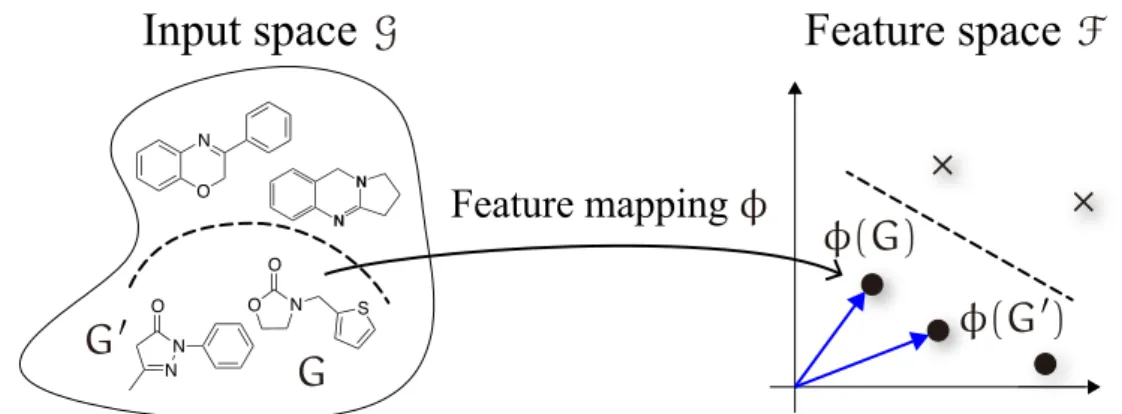
Traditionally, machine learning algorithms (e.g., support vector machine, logistic regres- sion, K-means clustering, etc.) have been well developed for the linear case. However, real-world problems often require nonlinear algorithms to detect the complex patterns that allow for the successful prediction of properties of interest. The use of a positive definite kernel^19,20 allows the extension of linear algorithms to nonlinear algorithms (Figure 2.1). The symmetric functionk : G×G → R on the domain G is said to be a positive definite kernel if and only if^∑i,j∈{1,...,n}^cicjk(Gi,Gj) ⩾ 0 for all n∈ N, G1^{, . . . ,}G_n∈ G, and c1^{, . . . ,}c_n∈ R. For suchk, it is known that a map ϕ : G→ F into a (usually high-dimensional) feature space F exists, such that k(G, G^′) =⟨ϕ(G), ϕ(G^′)⟩ for all G, G^′∈ G. In F, the complex patterns can be found as linear relations. Here, substituting k(G, G^′) for⟨ϕ(G), ϕ(G^′)⟩ is crucial for implicitly mapping the input data into F without ever knowingϕ(·). Any linear machine

Input space G Feature space F

O N

N N

O O N

O

S N

N

G

φ(G)

φ(G )

G

φ

Feature mapping

Figure 2.1 The idea of kernel methods. This approach maps the training data in the in- put space G into a high-dimensional feature space F via the feature map ϕ : G→ F, and applies linear machine learning algorithms such as SVM, which depend on the in- ner product ⟨ϕ(G), ϕ(G^′)⟩ between data points ϕ(G) and ϕ(G^′). Using the kernel trick k(G, G) =⟨ϕ(G), ϕ(G^′)⟩, it is possible to apply them without explicitly mapping ϕ.

learning algorithm formulated as an inner product in F can be turned into a nonlinear one by the kernel substitution, k(G, G^′) =⟨ϕ(G), ϕ(G^′)⟩. This approach is called the kernel trick. Next we review the nonlinear extension of support vector machines (SVMs) using the kernel trick.

Let us consider a typical binary classification task in chemical informatics as illustrated in Figure 2.1. The goal is to construct a discriminant function to predict whether a new input molecule is effective against a disease. Here, any molecule G in the set G of all molecules can be transformed into a feature vectorϕ(G)∈ R^p containing molecular prop- erties (e.g., molecular weight, molecular hydrophobicity, polar surface area, etc.). Suppose we are given the training data set D = {(ϕ(G_i), y_i)∈ X × Y}ⁿ_i=1where X is the nonempty set ofp-dimensional feature vectors and Y∈ {+1, −1} is the set of class labels whose value takes either the presence (+1) or absence (−1) of efficacy against the disease. Assume that D is separable, i.e., there exists a discriminant function f : G→ Y,

f(G) = sgn(⟨w, ϕ(G)⟩ + b), (2.1)

where the weight vector w∈ R^p and the shift coefficient b∈ R are parameters. SVM

2.1 Kernel Methods 12

determines the hyperplane, which separates the two classes with the largest margin, by solving the constrained optimization problem

minimize

w,b

1 2^||w||

2subject toy_i(⟨w, ϕ(G_i)⟩ + b) ⩾ 1 for all i = 1, . . . , n. (2.2)

Note that ||w||⁻¹f(G_i) is the distance from the point ϕ(G_i) to the hyperplane H(w, b) := {ϕ(G)|⟨w, ϕ(G)⟩ + b = 0}. The condition y_i(⟨w, ϕ(G_i)⟩ + b) ⩾ 1 ensures that the margin distance is at least 2||w||⁻¹. Consequently, minimizing ||w|| subject to the constraints max- imizes the margin of separation. To address this problem one can solve it in dual space, as follows. The Lagrange function of eq 2.2 is given by

L(w, b, α) =¹ 2^∥w∥

2₋

∑n i=1

α_i(y_i(⟨w, ϕ(G_i)⟩ + b) − 1), (2.3)

whereα_i^⩾0 is a Lagrange multiplier. L has to be minimized with respect to w and b and maximized with respect toα_i. At the saddle point, the derivatives ofL with respect to the variables w andb must be equal to zero,

∂

∂bL(w, b, α) = 0 and ^∂

∂wL(w, b, α) = 0,

which leads to

∑n i=1

α_iy_i= 0 (2.4)

and

w =

∑n i=1

α_iy_iϕ(G_i). (2.5)

Substituting eq 2.4 and eq 2.5 into the Lagrangian eq 2.3, we obtain the so-called dual

optimization problem

maximize

α_∈Rⁿ

W(α) =

∑n i=1

α_i−¹ 2

∑n i,j=1

α_iα_jy_iy_j⟨ϕ(Gi), ϕ(Gj^)⟩

subject toα_i⩾0 for alli = 1, . . . , n and

∑n i=1

α_iy_i= 0.

Using eq 2.5, the decision function (eq 2.1) can be written as

f(G) = sgn⁽

∑n i=1

y_iα_i⟨ϕ(G), ϕ(G_i)⟩

| {z }

k(G,Gi)

+ b⁾. (2.6)

Equation 2.6 can be expressed in terms of the kernel k using the kernel trick k(G, G_i) =

⟨ϕ(G), ϕ(G_i)⟩. The kernel trick allows us to handle the feature vectors ϕ(G) in the very high-dimensional feature space with no need to perform the explicit transformation,ϕ. To deal with structured data such as chemical structures, many graph kernels have been devel- oped, as described in Section 2.3. For further information on kernel-based machine learning please see the literature.^17–20

2.2 Representing Chemical Structures

Let us represent the chemical structure of a molecule by a labeled directed graph,G = (V, E), as shown in Figure 2.2. The graph G is described by a set of vertices V = {v_i}ⁿ_i=1 of size n = |V| representing the atoms in the molecule and a set of edges E = {(u, v)} ⊆ V × V representing the covalent bonds. Let ΣV^,ΣE be the sets of vertex labels and edge labels, respectively. In the case of labeled graphs, there is also a set of labelsΣ = ΣV∪ ΣE ^{with a}

labeling functionℓ : V∪ E → Σ that maps vertices and edges to corresponding element types and bond types, respectively. For directed graphs, each edge (u, v) is oriented and is a pair of the initial vertex u and the terminal vertex v. It is assumed that for every edge (u, v)

2.2 Representing Chemical Structures 14

N

N

O

(a) Chemical structure (b) Molecular graph

v₁

v₂ v₃

v₄

v₅ v₆ v₇

v₈ v₉ v₁₀

v₁₁ v₁₂

v₁₃

Figure 2.2 A chemical structure (left) can be modeled as a labeled directed graph (right).

belonging to E in G, the corresponding opposite edge (v, u) also belongs to E, i.e., G is symmetric. Such symmetric directed graphs can be viewed as undirected graphs. Note that V_G and E_Gwill be used to refer to the vertex and edge sets, respectively, of a specific graph G. We also define a function describing the outgoing neighbors (children) of a vertex v as N(v) = {u|(v, u)∈ E}.

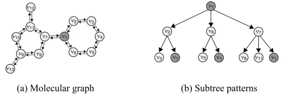
A rooted treeT = (V_T, E_T) is a directed acyclic graph with a single designated root, in which the edges have a natural orientation away from the root. The size |T | of the tree T is the number of vertices in T , i.e. |T | = |V_T|. The height h of the tree T is the length of the longest path from the root to any other vertex. Note that a vertex inG may appear several times in the tree-pattern, but sibling vertices in the tree-pattern must correspond to distinct vertices inG (see Figure 2.3).

v1

v2 v3

v₄

v5

v6

v7

v8

v9

v10

v11

v12

v13

(b) Subtree patterns (a) Molecular graph

v2

v₃ v₁ v5 v₁ v₈ v₁₁ v₁ v6

v1

v7

Figure 2.3 A molecular graph (left) and subtree patterns up to the heighth = 2 rooted at the nodev₁(right). Note that the vertexv₁appears at a height of 2 again.

2.3 Graph Kernels

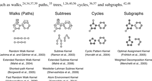
The traditional application of machine learning with the kernel method only considers data represented in a single row of a table. However, there are many potential machine learning applications, where this is not the natural representation. For example, such applications include the classification of molecules internally represented as graphs. The best known framework to construct kernels for structured data is the convolution kernel proposed by Haussler.³³ Following this framework, various graph kernels have been proposed over the last decade (see Figure 2.4) and applied successfully to various machine learning tasks in chemical informatics, including the establishment of QSARs. These graph kernels differ with respect to the choice of the subgraph types used to represent the structured objects, such as walks,24,34,37,39_paths,35_trees,1,26,40,56_cycles,36,57and subgraphs.^42,48

C O C C C

C C C C

N O

C N

C C

C

C C

C

C C C

Walks (Paths)

Random Walk Kernel (Kashima et al. and Gärtner et al., 2003)

Extended Random Walk Kernel (Mahé et al., 2004)

Fast Random Walk Kernel (Vishwanathan et al., 2006)

N O

C N

C C

C

C C

C

C C C

N O

N C

C

C C C

C C

Subgraphs

Optimal Assignment Kernel (Fröhlich et al., 2005) Weighted Decomposition Kernel

(Menchetti et al., 2005)

N O

C N

C C

C

C C

C

C C C

C C

C

C C C N

N C

C

C

Cycles

Cyclic Pattern Kernel (Horváth et al., 2004)

N O

C N

C C

C

C C

C

C C C

C C C C O

N C C

N C C

Subtrees

Subtree Kernel (Ramon et al., 2003)

Atom Environment Kernel (Yamashita et al., 2014) Weisfeiler-Lehman Subtree Kernel

(Shervashidze et al., 2009) Extended Subtree Kernel

(Mahé et al., 2006) Shortest-path Kernel

(Borgwardt et al., 2005)

Figure 2.4 The research efforts on graph kernels over the last decade.

2.3.1 Convolution Kernels

The basic idea of the convolution kernels³³is that each structured object is decomposed into a set of parts, and the kernel between the objects is defined as the sum of the kernel values

2.3 Graph Kernels 16

G G

s ∈ _S(G) s ∈ _{S(G )}

k

_{(s, s )}

N N O

O N O

S

...

O

N O

N N

S

O

O N O

O N

...

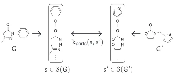
Figure 2.5 A schematic concept of the convolution kernel between the molecular graphsG andG^′.

among the parts (see Figure 2.5).

Let G, G^′ ∈ G be the molecular graphs and let S(G), S(G^′) be sets of parts extracted fromG, G^′. Given an extraction rule, we can define the sets S(G) and S(G^′) of parts. The convolution kernel ofG and G^′is then defined as

kconv(G, G^′) = ^∑

s∈S(G)

∑

s^′∈S(G^′)

w(s)w(s^′)kparts(s, s^′), (2.7)

where the function w(s) returns a weight for the part s and kparts(s, s^′) is the kernel func- tion between two parts s and s^′. Equation 2.7 is guaranteed to be a valid kernel if kparts

is a positive definite kernel. It should be noted that the weight function is not defined in the original definition.³³ The convolution kernel is very general and can be used for many different structured objects (e.g., amino acid sequences, chemical structures, metabolic net- works, etc.). To construct a convolution kernel for specific structured objects, we have to design the extraction rule of parts and the kernel function on the parts.

We next describe two established graph kernels: random walk kernels and subtree ker- nels.

2.3.2 Random Walk Kernels

The idea of the random walk (RW) kernel^24,34 is to randomly walk on two graphs and compare the label sequences resulting.

Consider a random walk on a graphG, which starts at vertex x₁∈ V_Gwith initial prob- ability p_s, goes from x_i−1 to x_i with transition probability p_t, and ends with probability p_q. The random walk can be represented as a sequence of the vertices traversed of lengthl, x = (x1^,x2^{, . . . ,}x_l). The vertex sequence x in G has probability

p(x|G) = p_s(x1)⁽

∏l i=2

p_t(xi^|xi−1⁾

)

p_q(xl^).

Let us define a label sequence by another alternating sequence of vertex labels and edge labels

h = (h1^,h2^{, . . . ,}h_2l−1)∈ (ΣVΣE^)l−1ΣV^.

We then obtain the label sequence associated with x

hx= (ℓ(x1)ℓ(x1^,x2), ℓ(x2), . . . , ℓ(x_l−1)ℓ(x_l−1,x_l), ℓ(x_l)).

The probability of the label sequence h is the sum of probabilities of all vertex sequences that generate h

p(h|G) =^∑

x

I(h ∼= hx^)·

( p_s(x1⁾

∏l i=2

p_t(x_i|x_i−1)pq(x_l)⁾,

whereI(h ∼= hx) is the indicator function that returns 1 if h and h_xare equal and 0 otherwise. Next, we define a kernel k_z between two label sequences h and h^′. Suppose we are given two valid kernels k_v between vertex labels andk_e between edge labels. The kernel

2.3 Graph Kernels 18

for the label sequences of equal length is given by the product of the label kernels

k_z(h, h^′) = kv(h1^,h1^′)

∏l−1 i=1

k_e(h_2i,h_2i^′)kv(h_2i+1,h_2i+1^′).

For the label sequences h and h^′ of different lengths, k_z(h, h^′) = 0. Finally, the random walk kernel is given by the expectation ofk_zover all possible h and h^′

kRW(G, G^′) =^∑

h

∑

h^′

k_z(h, h^′)p(h|G)p(h^′|G^′).

This kernel is positive definite for validk_vandk_e.

The RW kernel exploits an infinite dimensional feature space, spanned by random walks, on molecular graphs. In consequence, the RW kernel gives an alternative to explicit vector representations of molecules (molecular descriptors). However, Gärtner et al.³⁴ indicated the limited expressiveness of the RW kernel based on linear features. To alleviate this limi- tation, Gärtner et al.³⁴ proposed subtree kernels, as described in the next section.

2.3.3 Subtree Kernels

In this section we describe the subtree (ST) kernel initially proposed by Ramon and Gärtner¹ and later extended by Mahé and Vert.²⁶Following Mahé and Vert,²⁶we start by describing the concept of tree-patterns in a graph. LetG = (V_G, E_G) be a graph, and let T = (V_T, E_T) with V_T = (w1^{, . . . ,w}|T |) be a rooted tree with a designated root w1. A |T |-tuple of ver- tices (v₁, . . . ,v_{|T |}) ∈ V^{|T |}_G is said to be a tree-pattern of G with respect to T , denoted by

(v1^{, . . . ,}v_{|T |}) = pattern(T ), if and only if



















∀i ∈ {1, . . . , |T |}, ℓ(v_i) = ℓ(w_i),

∀(w_i,w_j)∈ E_T, (v_i,v_j)∈ E_G∧ ℓ((v_i,v_j)) = ℓ((w_i,w_j)),

∀(w_i,w_j), (w_i,w_k)∈ E_T, j̸= k ⇔ v_j̸= v_k.

(2.8)

With the set of all possible tree-patterns ofG = (V_G, E_G) with V_G= (v1^{, . . . ,}v_|VG|) arranged inT ,

P_{T(G) = {(va1}, . . . ,v_{a|T |})|(a1^{, . . . ,a}|T |⁾∈ {1, . . . , |V_G|}^{|T |}∧_(va1, . . . ,v_{a|T |}) = pattern(T )}, (2.9) the ST kernel of graphsG and G^′is given by

k_ST,h(G, G^′) = ^∑

T∈Th

µ(T ) ^∑

p∈PT(G)

∑

p^′∈PT(G^′)

I(p ∼=p^′). (2.10)

A set T_h of all trees up to heighth is considered. We assume that T_hincludes the elements of isolated vertices. For each tree T ∈ T_h, the sets of tree-patterns P_T(G) and PT(G^′) in- clude all tree-patterns occurring inG and G^′, which can be arranged in a given treeT . Each tree-pattern pair (p, p^′)∈ P_T(G)× P_T(G^′) is compared by the indicator function I(p ∼=p^′) that determines their isomorphism to be one ifp and p^′are isomorphic, and zero otherwise. In this case,I(p ∼=p^′) always returns one because both P_T(G) and P_T(G^′) include isomor- phic tree-patterns. Therefore, the ST kernel counts the weighted number of co-occurrences of tree-patterns inG and G^′. Each tree-pattern with respect toT has a weight µ(T ) depend- ing on the tree structure. A typical weight is a function of the tree size |T |, for example, µ(T ) = λ^{2|T |}, and assigns smaller weights to larger tree-patterns, whereλ is a nonnegative weight factor that is less than one. Alternative weights have been defined as functions of the structural complexity of the tree.²⁶

2.3 Graph Kernels 20

2.3.4 Other Graph Kernels

There have been various graph kernels proposed in the literature (see Vishwanathan et al.²¹). In this section, we discuss several important kernels in chemical informatics.

Walk-based kernels, one of the first graph kernels, have been independently proposed by Kashima et al.²⁴ and Gärtner et al..³⁴ Unfortunately, random walks on a graph include tottering between two neighboring vertices, which is otherwise known as an immediate re- visiting of a vertex. Such tottering walks are likely to be uninformative. Mahé et al.³⁷ introduced the second-order Markov model to filter tottering walks. Path-based graph ker- nels³⁵ have been proposed to invalidate the effects of tottering. Another extension³⁷ is to increase the number of different vertex labels using the Morgan index. In the label en- richment, contextual structural information around each vertex is embedded into the vertex label. Subsequently, Vishwanathan et al.³⁹ employed fast methods for solving Sylvester equations as well as conjugate gradient and fixed point iteration methods to speed up walk based kernels.

Ramon and Gärtner¹ defined kernels through the comparison of subtrees instead of walks on the graphs. This alleviates the limited expressiveness of linear features generated by random walks. The subtree kernel was later refined by Mahé and Vert.²⁶ Subsequently, the Weisfeiler-Lehman (WL) subtree kernel⁴⁰ was developed to provide an efficient ker- nel computation. The WL subtree kernel scales up to large labeled graphs. It uses the Weisfeiler-Lehman isomorphism test, which consists of iterative multiset-label determina- tion, label compression, and relabeling steps.

Horváth et al.^36,57 proposed cyclic pattern (CP) kernels, which are based on the idea of mapping graphs to the sets of cyclic patterns and tree patterns, which are compared with the intersection kernel. Menchetti et al.⁴⁸ proposed weighted decomposition kernels based on comparing local neighborhoods of vertices. The optimal assignment (OA) kernel,⁴² another graph kernel comparing local neighborhoods, arises from finding the best match

between substructures of graphs. However, the OA kernel is not positive semidefinite in general.⁵⁸ Vishwanathan et al.²¹ suggested a possible remedy to this problem based on an approximation of the tropical semiring.

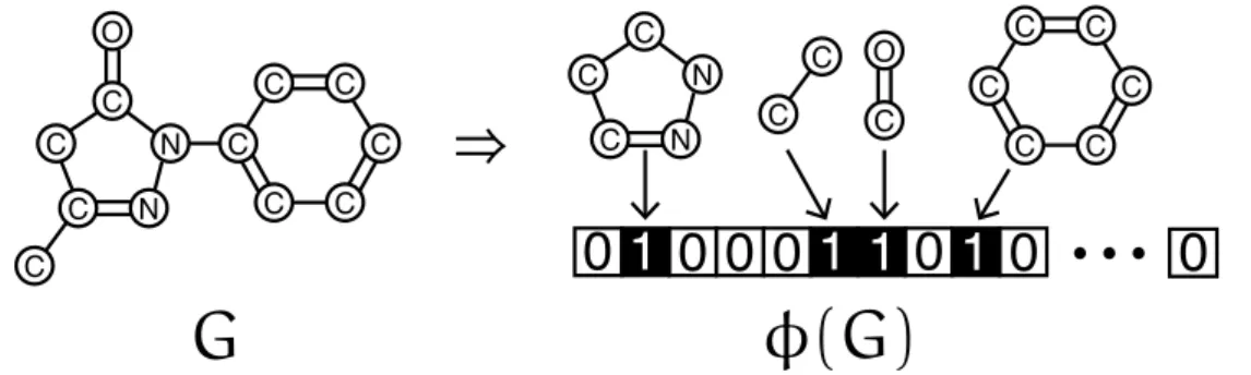
Other kernels, motivated by applications in chemical informatics, include fingerprint kernels^38,59 where a molecular graph G is represented by a vector ϕ(G) indexed by a set of molecular fragments as illustrated in Figure 2.6, i.e., sequences of atom types and bond types up to a given length. The fingerprint kernels are normalized by three variations of the Tanimoto kernel designed by analogy with the Tanimoto coefficient.

N O

C N

C C

C

C

C C

C C

C

・・・

0 1 0 0 0 1 1 0 1 0

O C

C C

C

C C

C C

C N

N C

C

⇒

0

G φ(G)

Figure 2.6 Given a molecule graphG, the traditional fingerprint is defined as a binary vector ϕ(G) such that it indicates the presence or absence of predefined particular substructures in G.

Chapter 3

Atom Environment Kernels for

the Forward Problem

3.1 Basic Idea

In this section we introduce two extensions to the ST kernel. The first extension, referred to as the inexact match extension, relaxes the requirement for exact tree-pattern matching by allowing matching between atoms with similar local environments, and the second ex- tension, referred to as the importance weight extension, introduces a tree weight function to adjust the contribution of each tree-pattern according to the overall statistical significance of the constituent atoms for a given task. For the inexact match extension, we alter the defi- nition of tree-patterns by omitting the first condition for the exact atom label matching from eq 2.8 as











∀(w_i,w_j)∈ E_T, (vi^,vj^{)∈ E}G^{∧ ℓ((v}i^,vj)) = ℓ((wi^,wj^)),

∀(w_i,w_j), (wi^,wk^{)∈ E}T^{, j̸= k ⇔ v}j^{̸= v}k^.

This alters the definition of the set P_T(G) in eq 2.9. Suppose we are given a tree-level kernel k_tree(p, p^′) to measure the similarity between tree-patterns p and p^′. The AE kernel is then

given by the weighted sum of ktree(p, p^′) over all possible pairs of tree-patterns induced fromG and G^′

k_AE,h(G, G^′) = ^∑

T∈Th

∑

p∈PT(G)

∑

p^′∈PT(G^′)

w(p)w(p^′)ktree(p, p^′), (3.1)

where T_h is a set of trees up to heighth, and w(p) is a weight associated with the tree- pattern p. In the following section we provide the constructions of the tree-level kernel k_tree(p, p^′) and the tree weight function w(p).

3.2 Inexact Match Extension

Consider a specific form of the tree-level kernelk_tree(p, p^′) between tree-patterns p and p^′

ktree(p, p^′) = ^∏

(v,v^′)∈A(p,p^′)

katom(e_r(v), er(v^′)).

The atom-level kernelkatom(e_r(v), er(v^′)) measures the soft similarity between atoms v and v^′through the atom environment labels e_{r(v) and er(v}^′). The atom environment label e_r(v) captures the local environment of each atomv in the molecular graph. As will be shown in section 3.5.1, e_r(v)∈ R^d (d = 2 in the present study) is derived from the modified Burden matrix⁴⁹ of a neighboring substructure of a topological radiusr centered at atom v. The tree-level kernelk_tree(p, p^′) measures the similarity of p and p^′as the product of the atom- level kernels over a set A(p, p^′) = {(p[i], p^′[i])}^|p|_i=1 of the aligned atom pairs ofp and p^′, wherep[i] is the ith element of a tuple p.

We construct a compactly supported (CS) kernel forkatomby multiplying the Gaussian kernel with a width parameterγ by a Wendland function⁶⁰

k_atom(e_r(v), er(v^′)) = ψ_d,c^{( ∥er(v) − er(v}

′_)∥

θ

)

exp(−γ∥e_r(v) − er(v^′)∥²). (3.2)

3.2 Inexact Match Extension 24

Gaussian 1.0

0.8

0.6

0.4

0.2

0

8 6

4 2

0

θ

1.0

0.8

0.6

0.4

0.2

0

8 6

4 2

0

Gaussian

(b) (a)

ψ⁽⁴⁾_2,0^×Gaussian ψ⁽⁴⁾_2,1^×Gaussian ψ⁽⁴⁾_2,2^×Gaussian

ψ⁽²⁾_2,1^×Gaussian ψ⁽⁴⁾_2,1^×Gaussian ψ⁽⁶⁾_2,1^×Gaussian

e_{r(v) − er(v )} e_{r(v) − er(v )}

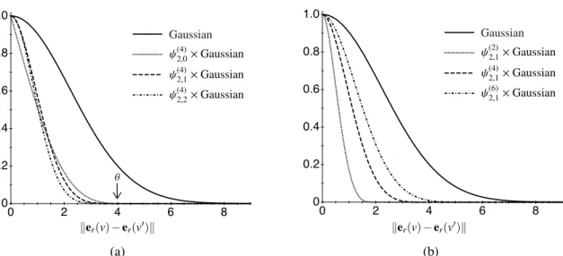
Figure 3.1 Plots of the Gaussian kernel with a width parameter of γ = 0.1 (solid line) and the CS kernelsψ^(θ)_2,c× Gaussian with respect to (a) the smoothing parameter c and (b) the cut-off distanceθ.

This construction has been proposed in a general machine learning context to yield a sparse Gram matrix without destroying the positive definiteness of any RBF kernel.⁶¹ The Wend- land functions ψ_d,c are defined for the dimension d of input variables and the smoothing parameter c, and tend to zero when the L₂ distance ||e_r(v) − er(v^′)|| is beyond a cut-off distance θ. With this construction, katom can smoothly decay to zero at θ without losing positive definiteness.⁶²

More specifically, the Wendland functions are defined as

ψ_d,c(z) = I^cψ_{⌊d/2⌋+c+1}(z), c = 0, 1, 2, . . . ,

with the truncated polynomial

ψ_s(z) = (1 − z)^s₊=











(1 − z)^s, 0 ⩽z < 1,

0, z ⩾ 1,

and the integral operator

I[f](z) =

∫_∞

z

xf(x)dx, z ⩾ 0,

where⌊·⌋ denotes the largest integer less than or equal to the argument, and I^cindicates the I-operator that is applied c times and transforms the function ψ_s to a smoother function. These functions are positive definite on R^d ford ⩽ 2s − 1. We can compute the functions ψ_d,cford = 2 and c = 0, 1, 2 directly by the explicit form⁶³

ψ2,0(z) = (1 − z)²₊,

ψ2,1(z) = (1 − z)⁴₊(4z + 1),

ψ_2,2(z) = (1 − z)⁶₊(1 + 6z +³⁵₃z²).

In Figure 3.1 the Gaussian kernel and the modified kernels with compact support using the Wendland functions ford = 2 with varying c and θ are shown. Since c is irrelevant to the sparsity ofψ_d,c as shown in Figure 3.1, we fixc = 0 in this thesis.

The compact support property ofk_atomeliminates the redundant matches between atoms that have intrinsically different local environments. This will ensure the detection of pairs of chemically meaningful tree-patterns in two molecular graphs.

3.3 Importance Weight Extension

Another important consideration is to determine the weight w(p) of a tree-pattern p. We assign an importance weight to each tree-pattern according to the overall statistical signifi- cance of the constituent atoms for a given classification or regression task.

In the case of a classification task, the chi-square (χ²) statistic is used to measure the statistical significance of the atoms. Each atomv is characterized by another atom environ- ment labela_r(v)∈ Z. As described later herein, ar(v) encodes information on a neighboring

3.3 Importance Weight Extension 26

Table 3.1 Two-way Contingency Table of Atom Environment Labela and Class Label c^a

c ^¬c ^∑row

a A B A + B

¬_{a C D C + D}

∑column A + C B + D N

aThe rows symbolize the presence and absence of the atom environment labela and the columns are the class labels (positive classc and negative class^¬c).

substructure of a topological radiusr centered at atom v using a Morgan type algorithm.³¹ Using a two-way contingency table (Table 3.1), where the rows signify the presence and ab- sence of the atom environment labela_r(v) = a and the columns are the class labels (positive class c and negative class^¬c), the association of a with the class labels can be evaluated with theχ²statistic

χ²(a) = ^{N(AD − BC)}

2

(A + C)(A + B)(B + D)(C + D)^,

whereA is the number of samples in which a and c co-occur, B is the number of samples in whicha occurs without c, C is the number of samples in which c occurs without a, D is the number of samples in which neitherc nor a occurs, and N is the total number of (training) samples. The value ofχ²(a) indicates the importance of atoms that have atom environment labela for the task of interest. Thus, the χ²statistic allows the identification of atoms with the ability to distinguish between two class labels. The weight of tree-patternp is then given by

w(p) =^∏

v∈p

w(aˆ _r(v))

with

w(aˆ _r(v)) =











λ_α, ifχ²(a_r(v)) ⩾ τ, λ_β, otherwise,

, 0< λ_β⩽λ_α< 1, (3.3)

whereτ is a χ² threshold. Onceτ is given, the significant atoms satisfying χ²(a_r(v)) ⩾ τ are determined and have weightλ_α, and the other atoms have a relatively small weightλ_β. The importance weightw(p) is expressed as the convolution of weight ˆw(a_r(v)) over the constituent atoms. The binarized atomic weights allows for easy visualization of significant atoms in a specific molecule, as seen in later.

In the case of a regression task, Welch’st-test is used to assess the statistical significance of each atom with atom environment label a. Given two groups 1 and 2 of observations from molecules with and without a, the association of a with the task can be assessed by thet-statistic

t(a) = ^{| ¯y1− ¯y2|}

(var(y1)/n1+ var(y2)/n2

)1/2^,

where ¯y_i, var(y_i), and n_i are the sample mean, sample variance, and sample size in the group i. Using t(a) instead of χ²(a) in eq 3.3, the tree weights for regression can be determined in the same manner as above.

For each tree-patternp, we denote the number of atoms found to be significant and less significant asn_α(p) and n_β(p), respectively. The AE kernel then becomes

k_AE,h(G, G^′) = ^∑

T∈Th

∑

p∈PT(G)

∑

p^′∈PT(G^′)

λⁿ_α^{α(p)+nα(p′)}λⁿ_β^{β(p)+nβ(p′)}

∏

(v,v^′)∈A(p,p^′)

k_atom(e_r(v), er(v^′)).

(3.4)

The atom-level kernels preserving positive definiteness are closed under tensor product and non-negative linear combinations.⁶⁴ The AE kernel is therefore positive definite.

In the case of unsupervised learning tasks, including cluster analysis and principal com- ponents analysis, the AE kernel could be applied by using prior knowledge on the impor- tance of the atoms. In the case where a given pharmacophore set (e.g., hydrogen-bond acceptor and donor, hydrophobic, etc.) is used, if an atom plays the pharmacophore role, the atom is given a higher weightλ_α. Alternatively, subject to a uniform weightλ_α= λ_βin