本文 Thesis 総合研究大学院大学学術情報リポジトリ A1757本文

(1)

Study on multi-timescale characteristics of

ionospheric trough in subauroral/auroral region

Tetsuro Ishida

Department of Polar Science,

School of Multidisciplinary Sciences,

The Graduate University for Advanced Studies

March 2015

(2)

1

Abstract

The F-region ionospheric trough is a band of depleted electron density that extends longitudinally around the nightside subauroral/auroral region of Earth. The averaged electron density structure of the trough is well known, but the physical and/or chemical processes associated with its structural variation are still unclear. Hence, a detailed and unified investigation within the trough region is highly desirable. To understand the fundamental characteristics of the trough region, we conducted a multi-part investigation that consisted of the following two steps.

For the first step, we investigated seasonal variation and solar activity dependence of the quiet-time ionospheric trough using plasma parameter data obtained via Common Program 3 (CP-3) observations performed by the European Incoherent Scatter (EISCAT) radar between 1982 and 2011. These statistical studies are based upon geomagnetically quiet to moderate conditions because we needed to understand the pure response of seasonal variation and solar activity dependence as the first step. The statistical results indicated that strong plasma flow plays an important role in the trough formation especially in the sunlit regions. Since frictional heating accompanied by strong plasma flow decreases electron density through dissociative recombination process, the trough can be preserved even during summer which has a relatively higher ionization rate than in the other seasons. We also found that such frictional heating becomes more intense under high solar activity, and thus the troughs with frictional heating tend to be deeper. Additionally, we propose the possibility that the occurrence rate of the trough was influenced by field-aligned currents (FACs). Some of the case studies previously reported that the downward FACs could produce the trough structure, but its statistical characteristic is still unclear. Thus, this is the first statistical study which mentioned the relationship between the trough and FACs. Especially during

(4)

3

equinox, the occurrence rate of the trough increased/decreased in the downward/upward current region with solar activity, which was possibly caused by solar activity dependence of the FACs intensity.

The statistical studies above were based upon geomagnetically quiet to moderate conditions, and thus, for the second step, analyses under geomagnetically active conditions were performed to further understand the basic characteristics of the trough. Specifically, we focused on the trough region during a substorm event and investigated the small-structure called an ionospheric blob (a few hundreds of kilometers in scale), which is considered to be the main source of the irregularities. As such small-scale structures vary over relatively short-term durations, and we conducted new EISCAT radar observations with high-speed meridional scans (60–80 s) during October and December 2013. The temporal evolution of a blob was observed during a substorm event on December 4, 2013. This is the first report regarding direct observations of blob deformation in the trough region during a substorm. The observational results indicated that the enhanced plasma flow was associated with the deformation process of the blob within the trough region. We suggest that the blob deformation was caused by the following two-step process: the initial “seed” density structures are created by the Kelvin–Helmholtz instability and dissociative recombination, and then the smaller scale irregularities are secondarily created by the gradient-drift instability.

In summary, the obtained results indicated that enhancement of plasma flow plays an important role in trough structuring over both long-term and short-term durations. In regards to the long-term duration, enhancement of plasma flow forms the trough through dissociative recombination and preserves its structure from the effect of ionization. Such trough structuring is more intense under high solar activity. In regards to short-term periods, enhancement of plasma flow also contributes to trough structuring in the form of blob deformation through dissociative recombination and

(5)

4

some of the plasma instabilities. Besides, the results also indicated that the occurrence rate of the trough was influenced by the FACs. Especially during equinox, the occurrence rate of the trough varied with solar activity possibly under the influence of solar activity dependence of the FACs intensity.

(6)

5

Acknowledgements

The author first would like to thank Dr. Yasunobu Ogawa (chief supervisor) and Dr. Akira Kadokura (sub-supervisor). They sincerely supported the author’s research activity and gave the author useful advice that helped him improve his research skills throughout the course of his Ph.D. work. Dr. Ogawa prepared the long-term EISCAT dataset necessary for the author’s research activities and thesis work. The research introduced in Chapter 3 is based upon this EISCAT dataset. He also provided the author with opportunities to attend the EISCAT observation campaign and many international conferences. The observational data obtained during this EISCAT campaign were used for the research presented in Chapter 4, and the knowledge obtained from the conferences is reflected in many parts of this thesis. The author would like to emphasize here that this thesis work could not have been accomplished without his sincere supervising and generous support. Dr. Kadokura also provided useful and constructive advice throughout the author’s Ph.D. activities. In particular, the discussion related to the magnetometer in Chapter 4 is based upon a series of discussions with him. Furthermore, he offered many helpful suggestions regarding the article from the perspective of magnetospheric physics.

The author also sincerely thanks Dr. Yasutaka Hiraki, Dr. Keisuke Hosokawa, and Dr. Yuichi Otsuka. Dr. Hiraki offered the author many helpful suggestions and much kind encouragement; discussions held with him are reflected in many parts of Chapter 3. Drs. Hosokawa and Otsuka also provided many helpful suggestions pertaining to the work presented in Chapter 4. The author also thanks Dr. Ryuho Kataoka for helpful suggestions regarding the research results. Additionally, the author wishes to express his heartfelt thanks to all staff members at the National Institute of Polar Research for their support and encouragement throughout his Ph.D. work.

(7)

6

This thesis research was supported financially by a Grant-in-Aid from the Japan Society for the Promotion of Science (JSPS) Fellows program. The author thanks Dr. Hiroshi Miyaoka for his employment as a research assistant. The author is indebted to the director and staff of EISCAT for providing the observational data. EISCAT is an international association supported by research organizations in China (CRIRP), France (CNRS, until the end of 2006), Finland (SA), Germany (DFG, until the end of 2011), Japan (NIPR and STEL), Norway (NFR), Sweden (VR), and the United Kingdom (NERC). In particular, Dr. Ingemar Häggström (EISCAT HQ) is also acknowledged for his helpful support in operating the EISCAT peer-reviewed program experiments and special experiments in Tromsø.

The author is thankful for the GPS-TEC data that were collected under the direction of A. J. Coster at the MIT Haystack Observatory. The TEC map was obtained from the GPS/TEC Plot routine on the Virginia Tech SuperDARN website (http://vt.superdarn.org/tiki-index.php?page=DaViT+TEC), which is supported by NSF award numbers AGS-0838219 and AGS-0946900. Additionally, the author thanks Dr. Takuya Tsugawa (NICT) and Dr. Michi Nishioka (NICT) for giving the author useful information about the TEC map.

The IMAGE magnetometer network is maintained by 10 institutes from Estonia, Finland, Germany, Norway, Poland, Russia, and Sweden. The author is grateful for their continuous effort in maintaining the instruments.

Finally, the author would like to express his sincere gratitude to the following advisory committee members for their constructive comments on this thesis: Dr. Yasunobu Ogawa, Dr. Akira Kadokura, Dr. Hisao Yamagishi, Dr. Keisuke Hosokawa, and Dr. Hitoshi Fujiwara.

(8)

7

1 Introduction

Here, we introduce the basic information necessary to understand this thesis. The basic physics of the upper atmosphere associated with this thesis is described in Sections 1.1–1.2. These sections are based upon Chapter 4 in Brekke [2013]. The basic information and some of the past publications of the ionospheric trough are introduced in Section 1.3. The plasma instabilities associated with the blob deformation (details are presented in Chapter 4) are explained in Section 1.4. Finally, we explain the objectives of this thesis in Section 1.5.

1.1 The upper atmosphere surrounding Earth

Earth’s atmosphere below ~100 km is composed of ~78.1% molecular nitrogen (N₂),

~20.9% molecular oxygen (O₂), ~0.9% argon (Ar), and ~0.1% other gases. Molecules start to dissociate above ~100 km of altitude, and the scale height of each chemical species is determined approximately by the equilibrium between the gravitational force and diffusion processes that depend on each species’ molecular mass. Hence, the constituents of the atmosphere vary with altitude. Figure 1.1 shows detailed altitudinal profiles of each species between 100 and 1000 km under solar minimum and maximum conditions [from U.S. Standard Atmosphere, 1976]. The dominant molecule/atom varies with altitude and solar activity. For example, atomic hydrogen dominates from 400–1000 km under solar minimum conditions (see Panel a), but atomic oxygen becomes dominant from 250–1000 km under solar maximum conditions (see Panel b). This occurs because the scale height of each species depends on atmospheric temperature, and thus, the scale height varies with solar activity. The neutral temperature varies with time of day, season, or solar activity, and the altitudinal profile of each species varies accordingly. In addition, it is known that atmospheric

(9)

8

composition has strong latitudinal dependence. Figure 1.2 shows the latitudinal dependence of molecular nitrogen (N₂), molecular oxygen (O₂), and helium (He) at 300 km under solstice and equinox conditions [from Roble, 1987]. In this figure, the important feature to note is that the O/N₂ ratio in the winter hemisphere is greater than that in the summer hemisphere. This latitudinal difference in atmospheric composition occurs because of the summer-to-winter neutral circulation, which is called the seasonal anomaly. The increased O and decreased N₂ densities in winter turn out to increase the O⁺ density. However, as the atmospheric composition is also influenced by chemical and physical processes, the situation is actually more complicated than described above. Some of the neutral atomic and molecular species turn into ions and electrons via photoionization processes in response to the Sun’s extreme ultra violet (EUV) radiation. The region where such ionization occurs is called the ionosphere (details below).

Beyond the limit of the ionosphere (~1000 km) is a region dominated by Earth’s magnetic field, which is called the magnetosphere. The plasma in the magnetosphere consists mainly of electrons and protons, which originate from the solar wind (from outer) and the ionosphere (from inner). There are small fractions of He⁺ and O⁺ ions of ionospheric origin and some He⁺⁺ ions originating from the solar wind. As the shape and boundary of the magnetosphere changes in response to the solar wind, its area cannot be delineated precisely. However, it has been confirmed from satellite observations that the sunward boundary of the magnetosphere is located ~10 Re from Earth (the distance between the dawn–dusk boundaries is ~15 Re) and its tail is elongated anti-sunward beyond ~150 Re (after Pilipp and Morfill [1987]; from Kivelson and Russell [1995]), as shown in Figure 1.3. Here, Re is the mean radius of the Earth

(= 6.37 × 10⁶ m). It is known that Earth is protected against cosmic rays and energetic particles from the Sun by the magnetosphere. In addition, the magnetosphere influences

(10)

9

the ionosphere via field-aligned currents (FACs). The spatial distribution of the FACs was first revealed by Iijima and Potemra [1976] using statistical analyses of satellite data. Figure 1.4 shows that the spatial distribution of the FACs (from Iijima and Potemra [1976]) comprises two current systems: Region 1 (R1) current and Region 2

(R2) current. The R1 current is distributed at the auroral region and located above the latitude of the R2 current. The R1 current flows outward from the ionosphere in the dusk sector and into the ionosphere in the dawn sector. Conversely, the R2 current flows into the ionosphere in the dusk sector and outward from the ionosphere in the dawn sector. It is considered that the magnetosphere and ionosphere form some sort of closed circuit via the FACs called the ionospheric current closure. Figure 1.5 shows a schematic image of the three-dimensional current closure in the magnetosphere–ionosphere (M–I) coupling system [after Hosokawa, 2008]. As electrons and ions play a role as carriers of current, it can be considered that this current closure influences the electron-density structure of the ionosphere. However, the physical and/or chemical processes associated with the M–I coupling are not fully understood. As the ionosphere is connected with the magnetosphere via geomagnetic field lines, magnetospheric convection is also mapped to the ionosphere in the M–I coupling system. Figure 1.6 displays how ionospheric convection is driven by the magnetosphere [after Hosokawa, 2008]. When the southward interplanetary magnetic field (IMF), i.e., the Sun’s magnetic field lines, contacts the terrestrial field lines at the dayside reconnection point (see D-Rx in Figure 1.6a), the IMF is reconnected with the terrestrial field lines and moves anti-sunward (see 1–6 in Figure 1.6b). Subsequently, the geomagnetic field lines become reconnected with each other at the nightside reconnection point (see N-Rx in Figure 1.6a) and move sunward via the outside trajectories (see 7–9 in Figure 1.6b). Hence, the signature of ionospheric convection is generally a two-cell pattern, as shown in Figure 1.6b. In the ionosphere, the

(11)

10

high-density plasma structures are convected from the dayside to the nightside, and their transport in the nightside region depends on the ionospheric convection pattern.

1.2 Ionosphere

The ionosphere is divided into three primary layers by altitude: the D-layer (70–100 km), E-layer (100–150 km), and F-layer (above ~150 km), although the F-layer is divided further into two distinct sublayers, the F1-layer (150–200 km) and F2-layer (above ~200 km), because of the strong EUV during daytime. The composition of the neutral atmosphere and EUV intensity vary with altitude, and thus, the predominant ion species and electron density also differ with altitude. Figure 1.7 shows the altitudinal profile of the most typical ion species together with the corresponding electron density profile [after Richmond, 1987; from Brekke, 2013]. This figure shows that the predominant ion species in the F region are O⁺ ions followed by NO⁺ ions and O₂⁺ ions. The neutral density is ~10¹⁵/m³ in the F region, while the electron density is at most ~10¹²/m³, even in daytime under solar minimum conditions. Hence, the ionization rate in the F region is at most ~0.1%. In addition, the electron density varies with time, season, or solar activity because the EUV intensity depends on these factors. Figure 1.8 shows the variation of the electron density profile with time and solar activity [from Richmond, 1987]. The electron density profiles for solar minimum and maximum conditions are similar, but the peak altitude clearly increases from solar minimum to maximum conditions. As mentioned above, because scale height increases with increasing temperature, the peak altitude also shifts upwards under solar maximum conditions.

The ion (electron) density in the ionosphere is held in equilibrium between the production by solar radiation and particle precipitation and the losses incurred by

(12)

11

chemical and photochemical processes and transportation phenomena such as diffusion, neutral winds, and plasma transportation caused by the FACs. This relationship can be expressed by the following continuous equation:

��i

�� ⁼^�ⁱ^{− �}ⁱ^{− � ∙ (�}ⁱ^�ⁱ⁾ ^(1.1)

where _�_i is the density of the ion species, _�_i is the production, _�_i is the loss by chemical and photochemical processes, and the last term is the divergence due to transportation phenomena through a volume of interest (the advection term).

First, we will explain the production term. The main causes of the production in the F region are solar radiation and particle precipitation from the magnetosphere. Among them, the production term caused by only solar radiation can be expressed with the following equation (e.g., see Chapter 4 in Brekke [2013] for the derivation of formula):

� = �_m,0^exp�1 − � − sec � exp(−�)� ^(1.2)

where _�_m,0 is the ion production rate at maximum for an overhead sun (χ = 0°), � is the solar zenith angle, and _{� = �� − �}_�,0_{� �}⁄ is the normalized height where �m,0^is

the altitude of peak production and � the scale height. Figure 1.9 illustrates the ionization profiles for different zenith angles between 0° and 80° [after Van Zandt and Knecht, 1964; from Brekke, 2013]. It can be seen that the height of peak production

increases with increases in the solar zenith angle. Furthermore, the peak altitude also becomes higher because of particle precipitation from the magnetosphere.

Next, we explain the loss term, which is most important regarding discussions of the ionospheric trough. As mentioned above, O⁺ ions are the dominant ions in the

(13)

12

ionosphere. It is known that O⁺ ions will combine with N₂ and O₂ molecules via the charge exchange reaction and produce NO⁺ and O₂⁺ ions with rate coefficients of _�₁ and _�₂, respectively:

O⁺+ N₂^�_{→ NO}¹ ⁺+ N O⁺+ O₂_{→ O}^�² ₂⁺+ O

(1.3)

The dissociative recombination occurs after the charge exchange reaction and as a result, the NO⁺ and O₂⁺ ions recombine with electrons as follows:

NO⁺+ e^�_{�� N + O}¹ O₂⁺ + e^�_{�� O + O}²

(1.4)

In a quasi-chemical photoequilibrium condition, the loss rate of electrons (dissociative reaction rate) is given by

� = ^�¹^[N²^{] +}^�²^[O²^] 1 + �_�¹

1

[N₂]

�_e ^{+ �}�²₂^[O�²_e^]

(1.5)

where [N₂] and [O₂] are the number density of N₂ and O₂, respectively. The values for _�₁ and _�₂ are on the order of 2 × 10⁻¹⁸m³s, while _�₁ and _�₂ are on the order of 10⁻¹³m³s. Furthermore, [N₂] < 10¹⁵m⁻³ and [O₂] _{≈ 10}¹⁴m⁻³ in the F-region altitude. Hence, _�₁_{∙ �}_e and _�₂_{∙ �}_e are respectively much larger than _�₁[N₁] and

�₂^[O₂], and thus, Equation 1.5 can be simplified as follows:

(14)

13

� = �₁^[N₂^{] +}�₂^[O₂^] ^(1.6)

The rate coefficients of dissociative recombination have been studied by many researchers [e.g., McFarland et al., 1973; Albritton et al., 1977]; hence, it is important to select appropriate coefficients for the targets. St.-Maurice and Torr [1978] parameterized the rate coefficient most suitable for the reaction of the high-latitude F region by using a bi-Maxwellian ion velocity distribution. Our research topic is the ionospheric trough in the high-latitude region, and therefore, we applied their rate coefficient for this study. The rate coefficients derived by St.-Maurice and Torr [1978] are expressed as follows:

�1 = 1.533 × 10⁻¹²− 5.92 × 10⁻¹³�₃₀₀^�^eff�

+8.60 × 10⁻¹⁴_�^�^eff

300� 300 ≤ �eff≤ 1700°�

(1.7)

�1 = 2.73 × 10⁻¹²− 1.155 × 10⁻¹²�₃₀₀^�^eff�

+1.483 × 10⁻¹³_�^�^eff 300^�

2

1700 <_�_eff< 6000°_�

(1.8)

�2 = 2.82 × 10⁻¹¹− 7.74 × 10⁻¹²�₃₀₀^�^eff�

+1.073 × 10⁻¹²_�^�^eff 300^�

2

− 5.17 × 10⁻¹⁴�₃₀₀^�^eff�³

+9.65 × 10⁻¹⁶_�^�^eff 300^�

4

300 <_�_eff_{≤ 6000°�}

(1.9)

where _�_eff (= (_�_i+_�_n) 2⁄ ) is the effective temperature, which is based on the ion temperature _�_i and neutral temperature _�_n.

In the ionosphere, the relationship between the ion-neutral temperatures and

(15)

14

ion-neutral relative velocities is expressed as follows (e.g., see Chapter 5 in Schunk and Nagy [2009] for the derivation of formula):

�i ⁼ �n⁺^�₃_�ⁿ⁽�i− �n⁾² ^(1.10)

where _�_n is the mean neutral mass, � is the Boltzmann constant, and (�i− �n^{) is}

the ion-neutral relative velocity.

For simplicity, assuming here that the neutral temperature and velocity do not change very much, we find that the enhanced convection flow leads to increased _�_i. This heating process caused by the enhanced convection flow is called frictional heating, which is considered to be the predominant heating process in the F-region ionosphere. Thus, the high-speed convective flow of the high-latitude ionosphere increases the _�_i because of frictional heating and that increased _�_i promotes dissociative recombination. Figure 1.10 shows a profile of the dissociative recombination rate � against the effective temperature. As shown in the figure, � increases with temperatures above

~1100 K, which indicates that frictional heating decreases electron density through dissociative recombination during high-speed convection.

1.3 Ionospheric trough

The ionospheric trough in the F region is characterized by a band of depleted electron density that extends longitudinally around the nightside subauroral/auroral region of Earth. Under geomagnetically quiet and moderate conditions, the overall trough structure is composed mainly of a high-latitude domain and a mid-latitude domain. Figure 1.11 shows the location of the quiet-time troughs [after Rodger et al., 1992]. In the high-latitude ionosphere, there are three regions of decreasing electron density: the

(16)

15

high-latitude trough (A), mid-latitude trough (B), and polar hole (C). In this paper, we focus on the high- and mid-latitude troughs. Here, we introduce the basic mechanisms of their generation and review past publications.

The high-latitude trough is usually accompanied by an increase in ion temperature (_�_i) caused by high-speed convective flow [e.g., Williams and Jain, 1986; Collis and Häggström, 1988], such that the trough is commonly regarded to form by dissociative

recombination accompanied by frictional heating. Additionally, the effects of upward ion flow (accompanied by frictional heating) on the high-latitude trough have also been investigated in relation to the overall trough-density structure [e.g., Winser et al., 1986]. As a result, many previous studies share a common interpretation that this mechanism alone cannot account for the observed drop in electron density in the F region [e.g., Williams and Jian, 1986; Winser et al., 1986].

Conversely, the mid-latitude trough is present in the subauroral region and it is generally considered to form via ordinary loss processes involving recombination in darkened regions of stagnated plasma flow (see red ellipse in Figure 1.11). Consequently, the mid-latitude trough is not accompanied by a similar increase in _�_i because no frictional heating occurs. Several researchers have studied the relationship between nighttime convection patterns and the formation of the mid-latitude trough. Spiro et al. [1978] proposed that this trough forms because of stagnation of plasma

around the duskside, where the return flow meets the co-rotating ionospheric plasma. Using a numerical convection model, Sojka et al. [1983] demonstrated that the mid-latitude trough forms in the nightside and extends past the terminator to the high-latitude dusk region. Furthermore, Whalen [1989] suggested that high-density plasma in the region of the dawn and dusk cells could be displaced by low-density nighttime plasma via sunward convective transport.

It has often been pointed out that small-scale structures or irregularities in the electron

(17)

16

density are produced within the trough region during geomagnetic active conditions, which affect the Global Navigation Satellite System (GNSS)-based navigation systems [e.g., Basu et al., 2008]. The Doppler and delay spread of HF signals, which are often caused by scattering or reflection from irregularities, are more frequent within the trough region during a sunspot maximum than during a sunspot minimum [Stocker and Warrington, 2011]. The scale size of the irregularities can range from tens of kilometers

down to hundreds of meters, and large-scale structures called “blobs,” in the scale length range of hundreds of kilometers, are considered to be the main source of the irregularities [e.g., Tsunoda, 1988]. However, the detailed process of their generation is still unclear because of the lack of adequate observations. Therefore, it is highly desirable that the processes associated with such small-scale structures within the trough be understood.

1.4 Plasma instabilities

The state of plasma fluid can be categorized roughly into the following two types: stable mode (or equilibrium) and unstable mode. The nature of this plasma stability can be explained through a simple analogy of a ball that is placed in a valley (stable state) or on the top of a hill (unstable state). If the ball is in the valley, from which no realistic perturbation can lift it away, the system is stable. After an initial perturbation, the ball returns to its equilibrium position. It may oscillate around the bottom of the valley for a long time if damping of the oscillation is weak. However, if the ball is at the summit of the hill, any perturbation will move it away from its position and the system is unstable. In such a situation, a small perturbation in the plasma fluid will grow or oscillate. Plasma instabilities grow by many types of mechanisms. In particular, it is known that the Kelvin–Helmholtz (K–H) instability and gradient drift (G-D) instability are

(18)

17

predominant in the high-latitude F region. As explained in Section 1.3, small-scale structures in the electron density are often observed within/around the trough region. Such structures are thought to be produced through the K–H instability and/or G-D instability around the trough region [e.g., Keskinen and Ossakow, 1983; Keskinen et al., 1988]. Here, we introduce the above two mechanisms that are associated with the discussion in Chapter 4.

The K–H instability is known to be the instability driven by the velocity difference (or flow shear) in the convection. As plasma convection exists in the polar ionosphere, the velocity differences in the plasma convection are observed inside and outside of the trough region. Hence, it is possible that such velocity differences influence the trough structure through the K–H instability. Figure 1.12 shows a schematic illustration of K–H instability in the high-latitude F region where the plasma flow is directed in the x-direction, an applied electric field is in the y-direction, a geomagnetic field line is in the z-direction, and L is the width of the shear region [after Keskinen et al., 1988]. Note that here we simplify the condition, although other factors such as the neutral wind are also involved in the real ionosphere. The linear growth rate of the K–H instability can be estimated from the work by Keskinen et al. [1988]. Accordingly, for ionospheric applications, the linear growth rate _�_KH can be expressed by the following equation:

�_KH^{= 0.2}∆� �⁄ ^(1.11)

Thus, the growth time _�_�� can be obtained by 5_{� ∆�}⁄ , which is the inverse of the growth rate. This means that the K–H instability grows more rapidly with stronger flow shear and narrower shear width.

Figure 1.13 describes a simplified schematic diagram of the G-D instability with a plasma density gradient directed in the x-direction, an applied electric field in the

(19)

18

y-direction, and a geomagnetic field line in the z-direction [from Tsunoda, 1988]. Given the above geometry, the positive feedback loop of the G-D instability operates as follows. When a perturbation pattern is imposed on the plasma density contours, the ions drift to the right along the background electric field _��⃗₀ (represented by the solid curve) leaving the highly magnetized electrons (dashed curve) behind. The resulting charge separation is accompanied by a polarization of the electric field _��⃗_�. The _��⃗_�×_��⃗ motion is in a direction such that the initial perturbation is amplified by moving plasma that is less dense further into regions of plasma that is more dense, and vice versa. Since the charge separation is produced through the large Pedersen mobility (mobility of the y-direction) of the ions as compared to that of the electrons, it becomes small in the F region where the Pedersen mobility of the ions is relatively small. As a result, the growth rate of the G-D instability is small in the F region.

1.5 Objectives of this thesis

Most previous studies on the trough have been based upon event investigations and statistical analyses that focus solely on electron density; thus, little is known about the predominant processes associated with trough formation on various time scales. In particular, the rapid temporal variation on a time scale of minutes within the trough region has not been investigated because of the lack of adequate observations. Therefore, there are many unsolved issues remaining in regards to the trough formation. Hence, the goal of this thesis was to develop an understanding of the processes associated with the trough’s structural change on several time scales, focusing especially on long-term (seasonal and solar activity) and short-term (60–80 seconds) variations.

The seasonal variation and solar activity dependence of the trough were investigated based upon the European Incoherent Scatter (EISCAT) radar dataset from 1982 to 2011, which encompasses about three solar cycles. In this research, we focused on the

(20)

19

variation of the trough’s occurrence rate and frictional heating accompanied by seasonal variation and solar activity dependence. The details of the approach used and the results obtained are described in Chapter 3.

The study on the rapid temporal evolution within the trough region required a new technique of Incoherent Scatter (IS) radar observation. Thus, we conducted new EISCAT radar observations as part of the Peer-reviewed Program (PP) and Japanese Special Program (SP) during October and December 2013, and we obtained data for nine events that each lasted for a period of 4 hours (14:00–18:00 UT, MLT_{≃ UT +} 2.2 h). In this research, we focused on localized plasma density enhancement, or so-called blobs, within the trough region, and then discussed the process of blob deformation. The details of the approach used and the obtained results are described in Chapter 4.

(21)

20

2 Instruments

This thesis reports on two major avenues of research (details are presented in Chapter 3 and Chapter 4), both of which have been conducted based on EISCAT radar data; however, other complementary observational data have been used. In this chapter, we introduce the instruments used in obtaining the data for this thesis work.

2.1 EISCAT radar

In general, observations by IS radars, including the EISCAT UHF radar system, are based upon Thomson scattering (see Section 6.1). The transmitter of the EISCAT UHF radar system is located in Tromsø, northern Norway (69°35'N, 19°14'E, Invariant Latitude: 66°12'N). Signals scattered from the ionosphere are received at stations in Kiruna, Sweden (67°52'N, 20°26'E, Invariant Latitude: 64°27'N) and Sodankyla Finland (67°22'N, 26°38'E, Invariant Latitude: 63°34'N), as well as at the transmitting site. In addition, another EISCAT radar is located in Svalbard, Norway (78°09'N, 16°03'E, Invariant Latitude: 75°10'N). Figure 2.1 shows the locations of the EISCAT radars.

From the spectrum shape of the IS signal, the plasma parameters (electron density, ion/electron temperature, and line-of-sight ion drift velocity) can be determined within the altitude range ~70–1000 km. We explain how the plasma parameters are determined from the spectrum shape of the IS signal in Section 6.2. By combining the line-of-sight ion velocities derived from the three stations that observe the same ionospheric volume, the three-dimensional ion velocity vector can be computed, and hence, the electric field that causes the E × B drift above ~200 km can be determined. As the trough usually stretches over a wide range of latitude, we used data from the meridional scanning observations of the EISCAT UHF radar. For the statistical analysis introduced in Chapter 3, we used the EISCAT Common Program 3 (CP-3) dataset that takes ~30

(22)

21

minutes for a single scan. The EISCAT CP-3 scan is a meridional scanning mode that follows a geomagnetic north–south trajectory during a single scan. Figure 2.2 shows a schematic illustration of the trough observed by the EISCAT CP-3 scan. Although this observational technique can follow relatively slow variations of the trough, such as seasonal variation or solar activity dependence, it is insufficient for observing more rapid temporal evolutions. Therefore, we used a high-speed meridional scan mode for the research, which is introduced in Chapter 4; its temporal resolution is 60–80 seconds, i.e., ~25 times higher than that of the CP-3 scans.

2.2 GPS-TEC

The Global Positioning System (GPS) is a measurement system composed of a constellation of 24 orbiting satellites. They emit continuous navigation signals on two different L-band frequencies (L1-band and L2-band) to ground-based GPS receivers. More than 1000 ground-based GPS receivers monitor the signals from the GPS satellites within their field of view, and thus, each GPS receiver can obtain the GPS signals in the visible area. A GPS signal is delayed during ionospheric propagation depending on the transmitting frequency and ionospheric electron density; therefore, from one transmission it is possible to obtain two delay times derived from the L1- and L2-band frequencies. As each individual delay time involves information regarding ionospheric electron density, we can calculate the total electron content (TEC) along the signal path from these two delay times. We introduce the details of the TEC calculation in Section 6.3.

As explained above, each GPS receiver can obtain the TEC value for each transmission, which means that we can construct maps of TEC values by combining data from the GPS receivers. Thus, the TEC maps alone can provide a large-scale

(23)

22

visualization of the temporal evolution of the ionospheric density structure. Figure 2.3 shows examples of the TEC maps [from Zhang et al., 2013]. The color scale runs from high-electron density (red) to low-electron density (blue). The dotted line across each panel is the day–night terminator at 100-km altitude. The blue circles and ellipses highlight the polar cap patch, the evolution of which is followed in this figure.

2.3 IMAGE magnetometers

The International Monitor for Auroral Geomagnetic Effects (IMAGE) consists of 31 magnetometer stations maintained by 10 institutes from Estonia, Finland, Germany, Norway, Poland, Russia, and Sweden. Figure 2.4 shows the locations of the IMAGE

magnetometer stations (see station information at

http://space.fmi.fi/image/beta/?page=maps). It is known that ionospheric currents accompanied by auroral activity flow in the E-region. As the ground magnetometers observe the geomagnetic variations caused mainly by the E-region Hall current, we can estimate the equivalent current from the magnetometer data [e.g., Iijima and Nagata, 1972]. Since the F-region drift vectors roughly go in the opposite direction from the E-region Hall current, we used data from the meridional chain stations to estimate the F-region drift vectors around the EISCAT observation range. Note that the perpendicular component of the field-aligned current and geomagnetic variation derived from the Pedersen current cancel out each other, and thus, the geomagnetic variation on the ground comes from only the Hall current in principle [Fukushima, 1976]. Hence, the estimated drift vectors from the IMAGE magnetometer can be used as a proxy of the real F-region convection.

(24)

23

3 Seasonal variation and solar activity

dependence of the quiet-time ionospheric

trough

3.1 Introduction

Statistical studies dealing with the seasonal variation of the trough can be found in a number of papers [Mallis and Essex, 1993; Horvath and Essex, 2003; Voiculescu et al., 2006; Lee et al., 2011]. For example, Lee et al. [2011] analyzed the seasonal dependence of the mid-latitude trough using the GPS Occultation Experiment data of FORMOSAT-3/COSMIC, which covers the period from February 2008 to January 2009, and showed that its electron-density structure changed dramatically in each season. Vo and Foster [2001] used Millstone Hill incoherent scatter radar data obtained between

1982 and 2000 to investigate the spatial extent and temporal evolution of the total electron content (TEC) at middle and subauroral latitudes. They showed that the latitudinal gradients in TEC associated with the equatorward wall of the trough are appreciably larger during a solar maximum than during a solar minimum. However, the processes responsible for the changes in the latitudinal gradients of the trough remain unclear.

As briefly mentioned in Section 1.3, radio propagation is affected by irregularities within the trough region. Stocker and Warrington [2011] reported that the Doppler and delay spread of HF signals, which are often caused by scattering or reflection from irregularities within the trough, are more frequent during a sunspot maximum than during a sunspot minimum. As these studies show that both electron density and the occurrence rate of the trough show significant variations depending on the season and solar activity, a detailed and unified investigation of these factors is required to fully

(25)

24

understand the trough’s basic characteristics.

In this chapter, we investigate the seasonal variation and solar activity dependence of the mid- and high-latitude troughs using an in-depth statistical analysis. Based on the EISCAT dataset from 1982 to 2011, which covers about three solar cycles, we then discuss the physical and chemical processes related to the evolution of the trough. To evaluate the occurrence rate of the trough (discussed later), we must differentiate the variation in the occurrence rate caused by seasonal variation and solar activity dependence from that caused by a change in the trough location. Given that the trough location changes according to auroral activity, whereby it shifts toward the equator as the Kp index increases [e.g., Moffett and Quegan, 1983; Rodger et al., 1992], we have used a dataset obtained under quiet and moderate geomagnetic conditions (Kp _{≤ 3-),} which can be considered as low auroral activity.

3.2 Data analysis

This study utilized a dataset obtained by the European Incoherent Scatter (EISCAT) UHF radar located in Tromsø, northern Norway (69°35'N, 19°14'E, Invariant Latitude: 66°12'N), which enabled us to observe ionospheric plasma parameters (electron density, ion/electron temperature, and line-of-sight ion drift velocity) in the altitude range of

~70–1000 km. In the present study, we must deal with all plasma parameters at the same altitudes, within the limitations of our statistical analysis; thus, we cannot eliminate the influence of hmF2 displacement accompanied by seasonal and solar activity variation. We used average plasma parameters between altitudes of 300 km and 350 km (near hmF2) to reduce the influence of hmF2 displacement. For long-term data analysis of the trough, we used the EISCAT dataset from 1982 to 2011, which covers about three solar cycles.

(26)

25

To visualize trough structures over a wide range of latitudes, we used scan data from EISCAT Common Program 3 (CP-3), as detailed in Table 3.1. This scanning mode follows a geomagnetic north–south trajectory during a single scan and covers a range of geomagnetic latitudes from approximately 73°N to 60.5°N at an altitude of 325 km. Since each scan takes ~30 min to complete, the EISCAT radar moves ~291 km eastward with the rotation of the Earth in non-rotating coordinates during a single scan. Therefore, 48 repetitions of the CP-3 scan obtain a physical quantity of plasma amounting to once around the earth. The different beam patterns and pulse codes used by the CP-3 scan are listed in Table 3.1. Its spatial resolution is dependent on these combinations, but all CP-3 scans can obtain a latitudinal distribution covering ~12.5° at an altitude of 325 km. The width of the ionospheric trough is generally less than 10° [e.g., Collis and Häggström, 1988], so we consider that either a part of or the entire trough can be

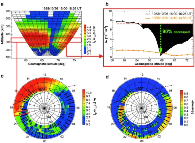
identified in the CP-3 scan data if the trough is located within the EISCAT field of view (FOV). An example of a trough measurement made by the CP-3 scan on October 26, 1988 is shown in Figures 3.1a–3.1c. Figure 3.1a shows the electron-density structure obtained from a single CP-3 scan on a dusk sector (16:00–16:26 UT). Here, the trough is characterized by a region of decreasing electron density around 67°N–69°N at an altitude of 250–500 km, represented by the dark-green/blue-colored grid squares. Figure 3.1b shows the latitudinal distribution of electron density (black line), which was derived by averaging electron density along the geomagnetic field line within the 300–350 km altitude range (red box in Figure 3.1a). Figure 3.1b contains a black shaded region that represents the extent of the trough, as determined using a detection algorithm (described below). A plausible background electron density (red dashed line in Figure 3.1b) was obtained by the following calculation. First, to determine the background electron density, we sorted the electron density values of the latitudinal distribution, generally 15–16 points, in ascending order. Then, we defined the median

(27)

26

value of the upper half of the data sequence obtained from the sorting process as the background electron density. We were able to determine a plausible background electron density in a situation where the latitudinal width of the trough was less than three-fourths of the scanning width. However, as this background electron density was identified solely by the latitudinal distribution of the CP-3 scan, it does not necessarily reflect the true value of the ionospheric background. These data show that the trough exhibits an electron density up to 90% lower than background levels, with a rate of decrease of ~30% per degree of latitude. In addition, the orange line in Figure 3.1b represents the electron-density variation measured at 14:40–14:56 UT on October 29, 1986, a similar time and month to the electron density data collected on October 26, 1988 (black line), but the orange-colored line was not detected at the trough as the solar zenith angle (SZA) is > 90°. This shows that the trough does not always form, even in regions with no sunlight. The rate of decrease along the orange line is ~11% per degree of latitude, which is, notably, only one-third of the rate of decrease for the trough itself (black line). We ignored gradual electron-density variations such as those shown by the orange line by considering them not as troughs, but as structures associated with diurnal variation.

We identified the trough region using a detection algorithm that exploits the fact that the trough, in particular the mid-latitude trough, is longitudinally elongated but latitudinally narrow. As a result, it covers several hours of magnetic local time (MLT), but only a few degrees of geomagnetic latitude (MLat). Therefore, we were able to identify the electron density variation in the trough by evaluating the latitudinal distribution, as shown in Figure 3.1b. We defined a region of decreasing electron density, the minima of which were at least 20% lower than the background value; this region was then identified as the trough region. Our data confirm that a 20% decrease is sufficient to distinguish the trough events from the non-trough events, with this value

(28)

27

able to detect trough events referred to in past studies [e.g., Collis and Häggström, 1988; Voiculescu et al., 2010]. Additionally, to verify this threshold, we showed that the trough characteristics detailed below (Section 3.3) did not change upon increasing this value, i.e., that the trough characteristics could be obtained using a threshold of just 20%.

Figure 3.1c shows the electron-density structure in MLT–MLat coordinates for the same day derived from 48 scans of the latitudinal distribution. Red-boxed regions indicate grid cells that correspond to the variation in electron density shown in Figure 3.1b. Dashed black lines represent the solar terminator, where SZA = 90°, and solid black lines indicate the latitudinal widths of the detected troughs. Here, the Altitude Adjusted Corrected GeoMagnetic coordinates (AACGM) system was used to calculate MLat. Note that we calculated MLT by using a simple conversion (MLT = UT + 2.5 hours) for ease of statistical analysis. Finally, Figure 3.1d shows the ratio of electron density decrease in the trough to the background electron density.

3.3 Results

Figure 3.2 shows the occurrence rates of the trough according to season and F10.7. These data have been divided into nine scenarios, each characterized by one of three seasons and one of three solar activities. For each grid cell, the occurrence rate (R) can be defined as follows:

R (MLT, MLat, F10.7, season) =n (MLT, MLat, F10.7, season)

N (MLT, F10.7, season) ^(3.1)

where n (MLT, MLat, F10.7, season) is the number of trough detections in each grid cell and N (MLT, F10.7, season) is the total number of events in each grid cell. The total

(29)

28

number of events N does not depend on MLat because one latitudinal distribution, i.e., a set of grid cells of that latitude, is used for one trough detection. Thus, the total number of events N is expressed as N (MLT, F10.7, season), not N (MLT, MLat, F10.7, season). Each annual period was divided into three periods (seasons): winter (±1.5 months around the winter solstice), summer (±1.5 months around the summer solstice), and the equinox (the remainder of the year). Note that Kp indices were limited to geomagnetically quiet and moderate conditions (Kp ≤ 3-), as explained in Section 3.1. These data show that the occurrence rate decreases from winter to summer (with decreasing SZA) for all solar activities. No data were available for winter during F10.7

= 180–300 solar flux unit (sfu) owing to the very limited number of samples. The occurrence rate appears to be maintained on the high-latitude side of the FOV (65°–72° MLat), even in the sunlit regions, whereas it is almost zero on the low-latitude side of the FOV (61°–65° MLat). Nevertheless, the relationship between the occurrence rate and F10.7 is not obvious, although it is clear that the occurrence rate varies with F10.7 in darkened regions.

As an example, Figure 3.3 presents the relationship between the occurrence rate and average description of the trough under the same conditions as in Figure 3.2e. In these figures, each panel indicates (a) the occurrence rate of the trough with overplotted ion drift velocity (_�_i) and (b) the ion temperature variation (_Δ�_i) in the trough. Red arrows shown in Figure 3.3a indicate eastward ion flows, whereas black arrows indicate westward ion flows. Each colored grid cell mapped on the polar plot has a resolution of 0.5 MLT and 0.6–0.8 MLat; however, grid cells containing fewer than four samples were displayed as blank areas. Note that most of the ion velocity vectors were calculated at heights of 275 km from tristatic observations, so the height of overplotted

�i is around 50 km below that of the occurrence rate and _Δ�_i.

Figure 3.3a shows that the strong eastward and westward flows exist on the

(30)

29

high-latitude side of the FOV, which are up to ~600 m/s. The value of _�_i tends to be smaller than ~100 m/s on the low-latitude side of the FOV. It appears that the occurrence rate increases up to ~80% along the return flow during 14:00–22:00 MLT, and additionally during 01:00–06:00 MLT. Moreover, it also increases up to ~80% in the region of small convection flow during 21:00–08:00 MLT on the low-latitude side of the FOV. Conversely, the occurrence rate decreases considerably down to ~10% during 22:00–01:00 MLT on the high-latitude side of the FOV, which is located approximately in the region of the Harang reversal (light blue in Figure 3.3a). The results also suggest that the occurrence rate is particularly low (< ~20%) during 00:00–07:00 MLT at 65°–67° MLat. Figure 3.3b demonstrates that _Δ�_i is greater than ~0 K on the high-latitude side of the FOV along the region of the return flow, but it is less than ~0 K on the low-latitude side of the FOV. Here, _Δ�_i in the trough is derived from the following simplified energy equations:

�_i ⁼�_n⁺^�ⁿ

3_�⁽^�ⁱ^{− �}ⁿ⁾

2 _{⟺ �}

i^−�n ⁼ ^�₃_�ⁿ⁽^�i^{− �}n⁾²

⟹ Δ�_i⁼ �_i−�_n ≃ �_{i (trough)}−�i (non−trough)

(3.2) (3.3)

where _�_n in a neutral temperature, _�_n is the mean neutral mass, � is the Boltzmann constant, and (_�_i_{− �}_n) is the ion-neutral relative velocity. We have presumed that _�_n is approximately equal to _�_i within the non-trough region in our statistical cases. Then, assuming that _�_n is equal to zero, _Δ�_i turns out to be nearly proportional to the square of _�_i, which is derived from Equation 3.2. Aruliah et al. [1996] demonstrated average neutral wind at the F region over Kiruna, Sweden, using the FPI dataset, which contains 9 years of observational data. According to their results, average neutral wind varies significantly around 0–100 m/s throughout the day under geomagnetically quiet to

(31)

30

moderate conditions. Thus, the error in _Δ�_i is within approximately ±100 K, even in the region of increased convection. On the whole, the _Δ�_i shown in Figure 3.3b increases with _�_i, providing support that the above assumption is reasonable. It is known that _�_i is typically increased in the high-latitude trough with frictional heating due to return flow, whereas it is not increased in the mid-latitude trough under geomagnetically quiet and moderate conditions [e.g., Moffett and Quegan, 1983; Williams and Jian, 1986; Ma et al., 2000]. Thus, it is considered that the region of

increased _�_i reflects frictional heating in the high-latitude trough. Note that _Δ�_i in the trough is not always smaller than ~0 K on the low-latitude side of the FOV because the mid-latitude trough also experiences significant frictional heating due to the subauroral polarization stream (SAPS) under geomagnetically active conditions, which spans the nightside from dusk to the early morning sector for all _�_p greater than 4 [e.g., Foster and Vo, 2002]. In our case, however, the primary source of increased _�_i is return flow located on the high-latitude side of the FOV because the occurrence rate of SAPS is low under geomagnetically quiet and moderate conditions.

3.4 Discussion

3.4.1 Seasonal variation

Figure 3.4 presents the seasonal variation in the ratio of the _Δ�_i within the trough (hereafter referred to as the _Δ�_i ratio), and the MLT distributions on both the high-latitude (upper panels) and low-latitude (lower panels) sides of the FOV are shown. Here, we defined the range of 65°–72° MLat and 61°–65° MLat as the high-latitude and low-latitude side of the FOV, respectively, as mentioned in Section 3.3. The left, middle, and right columns show the results for the winter, equinox, and summer seasons, respectively. The color bar has four sectors: blue (_Δ�_i < 200 �), yellow (Δ�i^{= 200}−

(32)

31

500 K), orange (_Δ�_i= 500− 1000 K), and red (Δ�_i ^{> 1000}�). Early studies used an increase in the F-region parallel _�_i exceeding 100 K to identify frictional heating events [McCrea et al., 1991; Davies et al., 1997]. However, the _�_i values deduced by incoherent scatter fitting typically contain error in the high-latitude trough region [Häggström and Collis, 1990]. Therefore, in the present study, we regard _Δ�_i _{≥ 200 K} as an indicator of frictional heating, since any error is within approximately ±100 K under geomagnetically quiet and moderate conditions. As seen in Figure 3.3b, the behavior of _Δ�_i is different between the high- and low-latitude sides; accordingly, we can discuss both sides separately.

The upper panels in Figure 3.4 show that the warm-colored bars (comprising yellow, orange, and red), which mean increased _�_i by frictional heating, are larger than ~85% in the post-midnight region (00:00–06:00 MLT) in all seasons. This means that a large part of the troughs are accompanied by large variations of _�_i produced by frictional heating of eastward return flow, as shown in Figure 3.3b. Figure 3.2 demonstrates that the occurrence rate is maintained at 80–90% in the post-midnight high-latitude region, even in summer, whereas it decreases significantly from winter to summer in other sectors. Hence, we conclude that dissociative recombination accompanied by frictional heating tends to cancel out any increases in the production rate due to increased solar EUV, such that the electron density trough can survive even in sunlit regions. In winter, however, the MLT distribution of the _Δ�_i ratio is not consistent with the occurrence rate shown in Figure 3.2. Increased _�_i is dominant near the midnight sector (21:00–06:00 MLT), whereas the occurrence rate of the trough increases in the dayside rather than the midnight sector. Therefore, it is possible that other physical and/or chemical processes are involved in controlling the trough formation, especially in darkened regions. Sojka et al. [1983] reported the results of numerical modeling of plasma transportation, which indicate that the duskside trough formed primarily owing

(33)

32

to transport of the nightside low-density plasma to the dayside. Thus, one interpretation of the discrepancy between the occurrence rate and the location of frictional heating during winter is that the plasma convection roughly determines the trough location, and consequently, it influences the occurrence rate. Another feature identified is the variation in the _Δ�_i ratio. In all seasons, increased _�_i is dominant near the midnight sector and it decreases toward the dayside. As shown in Figure 3.3a, the location of return flow moves to the outside of the poleward boundary of the FOV, which can lead to a decrease in the frictional heating rate from near the midnight to the dayside. Thus, it can be considered that _Δ�_i in the trough also decreases toward the dayside. Additionally, the ratio of increased _�_i decreases from winter to summer, with a particularly pronounced decreases (30–40%) in the dayside (e.g., 12:00–15:00 MLT; 09:00–12:00 MLT). The neutral density increases from winter to summer, which leads to an increase in the ion drag force on the neutral atmosphere; consequently, the term (_�_i_{− �}_n) of Equation 3.2 decreases, which leads to a decrease in _Δ�_i. Therefore, we suggest that an increase in the ion drag force on the neutral atmosphere from winter to summer causes a decrease in _Δ�_i in the trough.

The lower panels in Figure 3.4 demonstrate that the warm-colored bars decrease from winter to summer over all MLT sectors. Thus, it can be assumed that an increase in ion drag force from winter to summer suppresses an increase in _Δ�_i, as explained above. Furthermore, from the summer panels, it is clear that the sum of the warm-colored bars of the upper panel amounts to ~66% of the total; this proportion is ~47% greater than that of the lower panel. In other words, this indicates that there is a major difference in the ratio of frictional heating between the high- and low-latitude sides during summer. Furthermore, Figure 3.2 illustrates that the occurrence rate of the trough decreases down to ~10% on the low-latitude side of the FOV during summer. Therefore, we posit that the trough cannot survive without frictional heating in sunlit regions.

(34)

33

3.4.2 Solar activity dependence

Figure 3.2 shows that the occurrence rate varies with F10.7. To evaluate the variation in the occurrence rate in a more quantitative way, we compared occurrence rates in each season using values obtained by averaging all grid cells over a two-hour period (Figure 3.5) and plotted the MLT distribution of the occurrence on the high-latitude (upper panels) and low-latitude (lower panels) sides of the FOV. The left, middle, and right columns show the results for the winter, equinox, and summer seasons, respectively. The blue, green, and orange dotted lines shown in each panel denote the variation in the occurrence rate at F10.7 = 0–90 sfu, F10.7 = 90–180 sfu, and F10.7 = 180–300 sfu, respectively. The error bars indicate the standard deviation centered on the mean value.

During winter, when the darkened region covers the EISCAT FOV almost entirely, the occurrence rate changes little with F10.7 in the pre-midnight to post-midnight region (16:00–06:00 MLT), where it decreases significantly (by nearly 20–50%) with F10.7 in the dayside (07:00–16:00 MLT). It is reasonable to suppose that solar EUV makes a greater contribution to ionization for higher values of F10.7, thus leading to a decrease in the occurrence rate in the dayside. For the pre-midnight to post-midnight region, it is evident that the occurrence rate of the upper panel varies nearly symmetrically with that of the lower panel. The upper panel shows that the occurrence rate decreases down to

~20% within the pre-midnight region (18:00–00:00 MLT); this is ~30% lower than the rate in the midnight region (00:00 MLT). Conversely, the occurrence rate appears to increase up to ~80% in the post-midnight region (00:00–06:00 MLT), such that it is about 30% higher than that in the midnight region. In contrast to the upper panel, the lower panel of Figure 3.5 demonstrates that the occurrence rate increases up to ~80% within the pre-midnight region, such that it is ~30% higher than that in the midnight

(35)

34

region; conversely, it decreases down to ~20% in the post-midnight region, such that it is about 30% lower than that in the midnight region. Here, we presume that the increase/decrease in electron density accompanied by upward/downward field-aligned currents (FACs) can contribute to the formation of the F-region trough. Then, it can be assumed that the region 1 (R1) FAC causes the variation in occurrence rate in the upper panel, whereas the region 2 (R2) FAC causes that in the lower panel (red and blue shaded areas of winter in Figure 3.5). A relationship between the F-region trough and downward FACs has been indicated in some model works and observational evidence [e.g., Doe et al., 1995; Nilsson et al., 2005; Zou et al., 2013]. Thus, it is perhaps unsurprising that the increase/decrease in electron density caused by FACs could have an impact on the occurrence rate of the F-region trough.

Next, we focus on the occurrence rate in the equinox period. The upper panel of Figure 3.5 shows that the occurrence rate decreases by 20–30% with increasing F10.7 within the pre-midnight to post-midnight region (21:00–02:00 MLT), whereas it increases by 20–30% with increasing F10.7 within the post-midnight to morning region (02:00–07:00 MLT). Conversely, the lower panel shows that the occurrence rate increases by 30–40% with increasing F10.7 within the pre-midnight to post-midnight region and decreases by 40–50% with increasing F10.7 within the post-midnight to morning region. Subsequently, the occurrence rate varies with F10.7; consequently, the proportion of the occurrence rate is very similar to that in winter under high solar activity. Ohtani et al. [2014] showed that FACs are more intense during higher solar activity in the nightside. Therefore, it could be assumed that the variation in the occurrence rate with F10.7 during the equinox is a manifestation of solar activity dependence on FACs.

During summer, it can be recognized that the peak of the occurrence rate is located around 04:00 MLT in the upper panel of Figure 3.5. However, we cannot identify solar

(36)

35

activity dependence on the occurrence rate during summer. It is possible that high ionization rates in summer tend to suppress the formation of the trough, which presumably cancels out the solar activity dependence.

We also found that trough depth and frictional heating depend on solar activity. Figure 3.6 presents the MLT distributions of several parameters on the high-latitude side of the FOV, as in Figure 3.5: (a) trough depth and (b) _�_i within the trough. The trough depth is the ratio of electron density in the trough to the background electron density, as shown in Figure 3.1d. Figure 3.6a illustrates that the trough depth increases by 10–30% with increasing F10.7 within the post-midnight to morning (01:00–09:00 MLT) and dayside to duskside (12:00–16:00 MLT) regions during equinox, and within the midnight to morning region (00:00–09:00 MLT) during summer, as indicated by shaded areas. It is also clear that _�_i in the trough increases by 200–800 K with increasing F10.7 over the MLT sectors in which the trough deepens with increasing F10.7, as shown in Figure 3.6b. However, this characteristic is not obvious in winter. These data indicate that the trough becomes deeper via dissociative recombination caused by increased _�_i with increasing F10.7, at least during the equinox and summer seasons (but not winter). Now, focusing on the occurrence rate on the high-latitude side of the FOV during equinox (Figure 3.5), it can be seen that the post-midnight to morning region (02:00–07:00 MLT) where the occurrence rate increases with increasing F10.7 corresponds to the MLT sector where the trough depth and _�_i increases with increasing F10.7 (Figures 3.6a and 3.6b). As explained in Section 3.2, the regions of decreasing electron density, the minima of which were at least 20% lower than the background value, are detected in this study. Thus, the occurrence rate tends to be high within the region that the trough tends to become deep. In this respect, it can be considered that an increase of the occurrence rate within the post-midnight to morning region during equinox is caused by not only the FACs effect but also the enhanced dissociative