Evolution of a black ring by Hawking evaporation
Mitsuhiro Matsumoto
ABSTRACT
Black objects lose their mass and angular momenta through evaporation by Hawking radiation, and the investigation of their time evolution has a long his- tory. In this thesis, after reviewing previous studies on the time evolution of evaporating black holes, we study this problem for a five-dimensional doubly spinning black ring. We consider a thin black ring with a small thickness pa- rameter, λ ≪ 1, which can be approximated by a boosted Kerr string locally. For simplicity, we concentrate on the case in which the black objects emit only massless scalar particles. We show that a thin black ring evaporates with fixing its thickness parameter λ. Further, in the case of an Emparan-Reall black ring, we derive analytic formulas for the time evolution, which has one parameter to be evaluated numerically. By developing a numerical code, we determine the value of this parameter with sufficient numerical accuracy. We demonstrate that the lifetime of a thin black ring is shorter by a factor of O(λ2) compared to a five-dimensional Schwarzschild black hole with the same initial mass. We also evaluate the energy and angular spectra of radiated particles in the evapo- ration of a thin Emparan-Reall black ring. In addition to the evaporation of a thin black ring approximated by a boosted black string, we also discuss evap- oration of a thin five-dimensional unboosted Schwarzschild black string whose Schwarzschild radius 2MK is much smaller than the compactification scale L along the string direction. We study the time evolution of its mass and the en- ergy spectrum of emitted particle from the black string, and compare them with those of a four-dimensional Schwarzschild black hole. We show that the energy emission rate of a black string is larger by a factor of O(L/MK) compared to that of a black hole.
Contents
1 Introduction 3
2 Evolution of evaporating spherical black holes 5
2.1 Hawking radiation . . . 5
2.2 Evolution of a evaporating Kerr black hole . . . 10
2.3 Evolution of a evaporating Myers-Perry black hole . . . 13
3 Black rings 18 3.1 An Emparan-Reall black ring . . . 18
3.2 A Pomeransky-Sen’kov black ring . . . 21
4 Formulation 27 4.1 Emission rate . . . 27
4.2 Simplification . . . 28
4.3 Greybody factor . . . 30
4.4 Absorption cross section . . . 32
5 Evolution by Evaporation 35 5.1 Evolution of Pomeransky-Sen’kov black rings . . . 35
5.2 Evolution of Emparan-Reall black rings . . . 35
5.3 DeWitt approximation . . . 37
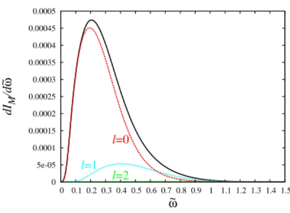
6 Energy and angular spectra 40 6.1 Formulas for energy and angular spectra . . . 40
6.2 Numerical results . . . 41
6.3 Spectrum of a five-dimensional thin black string . . . 45
7 Conclusion 53
1 Introduction
In four spacetime dimensions, a stationary, asymptotically flat, vacuum black hole is completely characterized by its mass and spin angular momentum[1]. In particular, the topology of its event horizon must be a sphere [2]. By contrast, in five dimensions, in addition to the Myers-Perry black hole [3] which is a natural generalization of the four-dimensional Kerr black hole, various exact solutions of black objects with nonspherical horizon topologies have been found [4, 5, 6, 7, 8](see [9] for a review). In this thesis, we focus attention to black ring solutions with the S1×S2horizon topology. A black ring solution rotating in the direction of S1 was found by Emparan and Reall [4]. Since a five-dimensional spacetime can have two angular momenta, Pomeransky and Sen’kov [10] extended it to a solution with two independent rotation parameters (i.e., spinning both in the directions of S1 and S2).
A black hole is known to evaporate due to quantum effects of fields in curved spacetime as shown by Hawking [11]. The rate of mass and angular momentum loss by the Hawking radiation for a Kerr black hole was first studied by Page [12, 13] taking account of fields with spins 1/2, 1, and 2, and it was shown that a Kerr black hole spins down to a nonrotating black hole regardless of its initial state. However, Chambers et al. [14] (see also [15]) showed that if only a massless scalar field is taken into account (i.e., in the absence of fields with nonzero spin), a four-dimensional Kerr black hole evolves to a state with the nonvanishing nondimensional rotation parameter, a/M ≃ 0.555. This analysis was extended to five-dimensional Myers-Perry black holes by Nomura et al [16]. They showed that any such black hole with nonzero rotation parameters a and b evolves toward an asymptotic state with a/M1/2= b/M1/2 ≃ 0.1975(8/3π)1/2. Here, this value is independent of the initial values of a and b.
It is interesting to extend these studies to the case of a black ring. Although the Hawking radiation of black rings has been studied in various context [17, 18, 19, 20], the time evolution of a black ring has not been studied up to now. The difficulty in this study is that the method of mode decomposition of the Klein-Gordon field in this spacetime is not known since separation of variables has not been realized, and therefore, two-dimensional numerical calculations of eigenfunctions are required. In order to avoid this difficulty, we consider a thin black ring with a small thickness parameter, λ ≪ 1. Here, “thin” or the small thickness parameter λ means that the S2 radius is much smaller compared to the S1 radius. In such a situation, a black ring can be approximated by a boosted black string. Then, the separation of variables for the scalar field can be done, and we have well defined modes.
Using this thin-limit approximation, we give a formulation to study the evolution of a thin Pomeransky-Sen’kov black ring by the Hawking radiation, and discuss general features that do not depend on details of the greybody factor. Then, we apply our method to a special case of the Emparan-Reall black ring without S2rotation, and derive a semi-analytic formula for the time evolution of the evaporation. Here, the formula is semi-analytic in the sense that the evolution is expressed by analytic formulas but they include one parameter
related to the greybody factors that have to be evaluated numerically. By developing a numerical code, we also determine the value of this parameter with sufficient numerical accuracy.
In addition to the time evolution, we present numerical results on detailed properties of the evaporation of a thin Emparan-Reall black ring. Specifically, we examine the energy and angular spectra of emitted particles in the evapo- ration. In order to clarify the property of the energy spectrum that is specific to the evaporation of a black ring, we discuss the results by comparing it with that of a four-dimensional Schwarzschild black hole.
Because a black ring was approximated by a black string in the thin-limit approximation above, we can apply our method also to evaporation of a thin black string. For this reason, we discuss evaporation of a thin Schwarzschild black string in the unboosted frame. Here, a thin black string means that the Schwarzschild radius 2MK is much smaller than the compactification scale L along the string direction. In addition to the formulas for time evolution, we present numerical results on detailed properties of evaporation such as an energy spectrum and compare them with those of a four-dimensional Schwarzschild black hole. We also discuss the connection of these results with the evaporation of a thin black ring.
This thesis is organized as follows. In Sec. 2, we review the evolution of a four-dimensional Kerr black hole and a five-dimensional Myers-Perry black hole. In Sec. 3, the black ring solution is reviewed and its boosted Kerr string limit is shown. In Sec. 4, we derive the equations that determine the emission rates of mass and angular momenta of a black ring via Hawking radiation. In Sec. 5, the time evolution of evaporating black rings is discussed and we check the validity of our numerical result by studying the DeWitt approximation. In Sec. 6, we present the energy and angular spectrum of emitted particles in the evaporation of a thin Emparan-Reall black ring. In addition, we discuss evaporation of a thin Schwarzschild black string. Sec. 7 is devoted to a conclusion. To simplify the notation, we use the natural units ℏ = c = kB= 1.
2 Evolution of evaporating spherical black holes
In this section, we review the evolution of black holes with spherical horizon by Hawking evaporation. In the first subsection, we explain Hawking radiation. In the remaining two subsections, the time evolution of a Kerr black hole and a Myers-Perry black hole, emitting massless scalar particles, is discussed.
2.1 Hawking radiation
Black holes do not only absorb matter around them, but also emit radiation with a thermal spectrum due to quantum effects, which is called Hawking ra- diation. We derive the thermal spectrum, following the discussion in Ford’s lecture note[21].
2.1.1 Particle creation
We consider a massless scalar field satisfying the Klein-Gordon equation in curved spacetime
(−g)−1/2∂µ(√−ggµν∂νΦ) = 0, (2.1) where g is the determinant of the metric gµν. We define the inner product of a pair of solutions of the Klein-Gordon equation by
(f1, f2) = i
∫
(f2∗∂µf1− f1∂µf2∗)dΣµ, (2.2) where dΣµ = dΣ nµ. Here, dΣ is the volume element in a given spacelike hypersurface, and nµ is the timelike unit vector normal to this hypersurface.
Let {fj, fj∗} be a complete set of solutions of Eq. (2.1), where fj has a positive norm. We write the field Φ using annihilation and creation operators aj and a†j′ as
Φ =∑
j
(ajfj+ a†jfj∗). (2.3)
The commutation relation is [aj, a†j′] = δjj′ and a vacuum state |0⟩ is defined by aj|0⟩ = 0.
Let us consider a spacetime which is asymptotically flat in the past and in the future, but which is non-flat in the intermediate region. Let {fj} be positive frequency solutions in the past (the “in-region”), and let {Fj} be positive fre- quency solutions in the future (the “out-region”). These modes are orthonormal in the sense that
(fj, fj′) = (Fj, Fj′) = δjj′, (fj∗, fj∗′) = (Fj∗, Fj∗′) = −δjj′, (2.4) with all other inner products vanishing. We expand the in-modes in terms of the out-modes:
fj =∑
k
(αjkFk+ βjkFk∗). (2.5)
From Eq. (2.4), we have the conditions for αjk and βjk.
∑
k
(αjkα∗j′k− βjkβj∗′k) = δjj′, ∑
k
(αjkαj′k− βjkβj′k) = 0. (2.6)
The inverse expansion is
Fk=∑
j
(α∗jkfj− βjkfj∗). (2.7)
The field Φ can be also expanded in terms of {Fj}. Φ =∑
j
(bjFj+ b†jFj∗). (2.8)
The aj and a†j are annihilation and creation operators, respectively, in the in-region. On the other hand, the bj and b†j are the corresponding operators for the out-region. The in-vacuum state is defined by aj|0⟩in= 0, whereas the out-vacuum state is defined by bj|0⟩out = 0. These creation and annihilation operators are related to each other:
aj=∑
k
(α∗jkbk− βjk∗ b†k), bk=∑
j
(αjkaj+ βjk∗ a†j). (2.9)
This relation is called a Bogolubov transformation, and the αjk and βjk are called the Bogolubov coefficients.
In the following, we will consider the gravitational collapse. Namely, the in- region is described by the past null infinity I−, and the out-region is described by the future null infinity I+ and the future event horizon H+. The number operator which counts particles on I+ is Nℓ= b†ℓbℓ, where ℓ is the mode which left I− and reached I+, not H+. Thus the mean number of particles created into mode ℓ is
⟨Nℓ⟩ =in⟨0|b†ℓbℓ|0⟩in=∑
j
|βjℓ|2. (2.10) If any of the βjℓcoefficients are non-zero, the particle creation occurs.
2.1.2 Thermal spectrum
For simplicity, we wil concentrate on the case of a massless scalar field in a four-dimensional nonrotating black hole, i.e., a Schwarzschild black hole. The metric of a Schwarzschild black hole is given by
ds2= −f(r)dt2+ dr
2
f (r)+ r
2dΩ2, (2.11)
where
f (r) = 1 −2G4rMS, dΩ2= dθ2+ sin2θdϕ2. (2.12)
Here, G4 is the four-dimensional gravitational constant and MS is the mass of the Schwarzschild black hole. Its event horizon is located at r = 2G4MS. For later use, we define the advanced and retarded time coordinates as
v = t + r∗, u = t − r∗, (2.13) where r∗ is the tortoise coordinate given by
r∗= r + 2G4MS ln( r − 2G4MS 2G4MS
)
. (2.14)
We imagine that the black hole was formed at some time in the past by gravitational collapse, and assume that no scalar particles were present before the collapse began. The in-modes, fωℓm, are pure positive frequency on the past null infinity I−, so fωℓm∼ e−iωv as v → −∞, Similarly, the out-modes, Fωℓm, are pure positive frequency on the future null infinity I+, so Fωℓm∼ e−iωu as u → ∞. In order to determine the particle creation, we need to calculate the Bogolubov coefficients.
In WKB approximation, the out-modes asymptotically behave as
Fωℓm∼
Yℓm(θ, ϕ)
√4πω r ×
{e−iωu, on I+
A(ω)e4G4MSiω ln[(v0−v)/C], on I− (2.15) where Yℓm(θ, ϕ) is a spherical harmonic, C is a constant, and v0 is the limit- ing value of v for rays which pass through the body before the horizon forms. Therefore, the out-modes on I− have the form
Fωℓm∼
{A(ω)e4G4MSiω ln[(v0−v)/C], v < v0
0, v > v0
(2.16)
We expand out-modes in terms of in-modes: Fωℓm=
∫ ∞
0
dω′(α∗ω′ωfω′ℓm− βω′ωfω∗′ℓm). (2.17) Here we did not write the common modes (ℓ, m) of the Bogolubov coefficients α∗ω′ℓm,ωℓm and βω′ℓm,ωℓm. Thus, βω′ωis
βω′ω= −2π1 √ ωω′A(ω)
∫ v0
−∞
dv e−iω′ve4G4MSiω ln[(v0−v)/C]
= −2π1 √ ωω′A(ω)eiωv0
∫ ∞
0
dv′eiω′v′e4G4MSiω ln(v′/C),
(2.18)
!"
#$
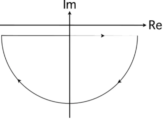
Figure 1: The closed contour of the integration in Eq. (2.20).
where v′= v0− v. On the other hand, α∗ω′ω is
α∗ω′ω= 1 2π
√ ω′ ωA(ω)
∫ v0
−∞
dv eiω′ve4G4MSiω ln[(v0−v)/C]
= 1 2π
√ ω′ ωA(ω)e
iωv0
∫ ∞
0
dv′e−iω′v′e4G4MSiω ln(v′/C)
= −2π1 √ ωω′A(ω)eiωv0e4πG4MSω
∫ ∞
0
dv′eiω′v′e4G4MSiω ln(v′/C).
(2.19)
Here, we use
I
C
dv′e−iω′v′e4G4MSiω ln(v′/C)= 0, (2.20) where the integration is taken around the closed contour C illustrated in Fig. 1. From Eq. (2.18) and Eq. (2.19), the Bogolubov coefficients are related to each other as
|αω′ω| = e4πG4MSω|βω′ω|. (2.21) The condition on the Bogolubov coefficients, Eq. (2.6), is written as
∑
ω′
(|αω′ω|2− |βω′ω|2)=∑
ω′
(e8πG4MSω− 1)|βω′ω|2= 1. (2.22)
The mean number of particles created into mode (ω, ℓ, m) is now given by
⟨Nω,ℓ,m⟩ =∑
ω′
|βω′ω|2= 1
e8πG4MSω− 1. (2.23)
This is a thermal spectrum with a temperature of TS= 1
8πG4MS
(2.24) which is the Hawking temperature of the black hole.
This discussion can be extended to the case of D(> 4) dimensional nonrotat- ing spherical black holes. The difference is that instead of ω and TS, we need to use the energy of a scalar particle in the background of a D-dimensional nonro- tating spherical black hole and the temperature of the horizon. In the rotating case, we have to replace ω by the energy ω∗ of the mode with respect to the null geodesic generator of the black hole horizons because the mode function behaves as exp(−iω∗u±) in the coordinates that are regular around the black hole horizon, where u± is the advanced time/retarded time around the horizon. In general, this null geodesic generator ξ can be written as ξ = ∂t+∑jΩj∂ϕj in terms of the time translation Killing vector ∂tand the rotational Killing vectors
∂ϕj. From this, it follows that ω∗ for the mode ∝ exp(−iωt + i∑jmjϕj) is
expressed as
ω∗= ω −∑
j
mjΩj. (2.25)
2.1.3 Greybody factor
Particles emitted from a black hole traverse a curved spacetime geometry before they reach an observer located at infinity. The black hole background thus work as a potential barrier for them and give a deviation from the blackbody radiation. Though particles emitted with sufficiently high energy reach the observer, particle emitted with law energy go back to the black hole by its gravitational pull. Therefore, the accurate expected number of particles emitted per unit time for each mode for a Schwarzschild black hole is given by
⟨NS⟩ = Γ
(Sch) ℓm (ω)
eω/TS − 1, (2.26)
where Γ(Sch)ℓm (ω) is a deviation from the blackbody radiation, called greybody factor. The greybody factor is the probability for an outgoing wave of the cor- responding modes to reach infinity. Owing to the flux conservation, this coin- cides with the absorption probability of the incoming wave of the corresponding modes.
Next, we formulate the time evolution of the black hole mass. Particles emitted in a time interval ∆t have the following discrete energy:
∆ω = 2π
∆t× (natural number). (2.27)
The energy of the particles emitted in ∆t for each mode is therefore
∆E
∆t =
∆ω
2πω⟨NS⟩. (2.28)
Because the total energy can be obtained if we take summation of Eq. (2.28) over all modes, the emission rate of the mass of the black hole is formulated as
−dMdtS = 2π1 ∑
ℓm
∫ ∞
0 ω⟨N
S⟩dω, (2.29)
where the summation is taken over all modes. In order to determine the time evolution of a black hole in Hawing radiation, we need to obtain the greybody factor for each mode, which has to be evaluated numerically.
2.2 Evolution of a evaporating Kerr black hole
We discuss the evolution of a Kerr black hole emitting scalar radiation via the Hawking process [14] (see also [15]) .
2.2.1 Kerr solution
The metric of a Kerr black hole is given in the Boyer-Lindquist coordinates as ds2= −
(
1 −2G4MKr ρ2
)
dt2−2G4MKar sin
2θ
ρ2 (dtdϕ + dϕdt) +ρ
2
∆dr
2+ ρ2dθ2+sin2θ
ρ2
[(r2+ a2)2− a2∆ sin2θ]dϕ2,
(2.30)
where ρ2 = r2 + a2cos2θ and ∆ = r2 − 2G4MKr + a2. MK and a corre- spond to the mass and rotational parameter, respectively. One can recover the Schwarzschild metric (2.11) by setting a = 0. The event horizon is located at r = r+ where
r±:= G4MK±
√
G4MK2 − a2= G4MK(1 ±√1 − a2∗), (2.31) with a∗:= a/(G4MK). The temperature and surface gravity of the horizon are
TK= κK
2π, κK =
r+− r−
4G4MKr+. (2.32)
We transform the Boyer-Lindquist coordinates (2.30) to the Kerr ingoing coordinates (v, r, θ, ˜ϕ). Here, (v, ˜ϕ) are introduced as
dv = dt + (r2+ a2)dr
∆, d ˜ϕ = dϕ + a dr
∆. (2.33)
With these coordinates, the Kerr metric in the Kerr ingoing coordinates is given by
ds2= − (
1 −2G4ρM2Kr )
dv2−2G4MKar sin
2θ
ρ2
(d ˜ϕdv + dvd ˜ϕ)
− 2a sin2θd ˜ϕdr + 2drdv + ρ2dθ2 +sin
2θ
ρ2
[(r2+ a2)2− a2∆ sin2θ]d ˜ϕ2
(2.34)
2.2.2 Formulation
We formulate the emission rate of the mass and angular momentum of the Kerr black hole, following Page[13].
In terms of Kerr-ingoing coordinates (v, r, θ, ˜ϕ), the Klein-Gordon equation
□ϕ = 0, separates by writing ϕ = R(r)S(θ)e−iωveim ˜ϕ, where the angular func- tion S(θ) is a spheroidal harmonics. The radial function, R(r), satisfies
[ d dr∆
d dr− 2iK
d
dr − 2iωr − λ ]
R(r) = 0, (2.35)
where K = (r2 + a2)ω − am, λ = Eℓmω− 2amω + a2ω2, and Eℓmω is the separation constant. Asymptotic solutions can be expressed by
R −→{ ZZhole r → r+,
inr−1+ Zoutr−1e2iωr r → ∞. (2.36) The subscript “in” refers to an ingoing wave originating from infinity, “out” refers to an outgoing wave reflected from the black hole that propagates toward infinity, and “hole” refers to the component of the wave that is transmitted into the black hole through the horizon at r = r+. The greybody factor Γ(Kerr)ℓm (ω) is
Γ(Kerr)ℓm (ω) = 1 −
Zout
Zin
2
. (2.37)
We express the rates at which the mass and angular momentum decrease by the quantities
f := −MK2M˙K, g := −MK
a∗ J˙K. (2.38)
where the dot ( ˙ ) denotes the derivative with respect to t. This definitions remove overall dependence on the size (mass) of the black hole. The coordinate t is the usual Boyer-Lindquist time coordinate. These quantities will determine the evolution of the Kerr black hole, which is defined by
( f g
)
=∑
l,m
1 2π
∫ ∞ 0
dx Γ
(Kerr) ℓm (ω)
e(ω−mΩK)/TK− 1
( x
ma−1∗ )
. (2.39)
Here ΩK = a∗/2r+ is the surface angular frequency, and we have defined x = MKω. The relative magnitude of the mass and angular momentum loss rates will determine whether or not the black hole will spin down to a nonzero value of a∗. To obtain the evolution of a∗, we differentiate a∗= JK/MK2 with respect to time t. From Eq. (2.38), the equation for a∗ is derived as
˙a∗ a∗ = −
hf
MK3 , (2.40)
where h(a∗) was defined by
h(a∗) := g(a∗)
f (a∗)− 2. (2.41)
6.0e-05 8.0e-05 1.0e-04 1.2e-04 1.4e-04 1.6e-04 1.8e-04 2.0e-04 2.2e-04 2.4e-04 2.6e-04 2.8e-04
0 0.1 0.2 0.3 0.4 0.5 0.6 0.7 0.8 0.9 1
f
a*
0 1.0e-04 2.0e-04 3.0e-4 4.0e-04 5.0e-04 6.0e-04 7.0e-04
0 0.1 0.2 0.3 0.4 0.5 0.6 0.7 0.8 0.9 1
g
a*
Figure 2: The scale invariant mass(left panel) and angular momentum(right panel) loss rates, due to scalar particle emission, for a Kerr black hole. In the left panel, the mass loss rate approaches the value 7.439 × 10⁻⁵at low rotation, while it reaches 2.601 ×10⁻⁴at the extreme limit a∗= 1. In the right panel, the angular momentum loss rate approaches 8.886 × 10⁻⁵ at low rotation, while the emission rate is 6.853 × 10⁻⁴ at a∗= 1. These figures are taken from Ref. [14].
When h = 0, Eq. (2.40) becomes ˙a∗ = 0. This means that the Kerr black hole continues to lose mass with a nonzero constant value, a∗= a∗0. Since the mass loss rate is always positive throughout the Hawking process, the function f must be positive definite. If dh/da∗ is positive at a point where h = 0, the black hole will asymptotically evolve toward a stable state. If dh/da∗is negative or zero at the point, then it represents an unstable equilibrium point of a∗, and the black hole will evolve away from it.
2.2.3 Results
In Ref. [14], Chambers et al. numerically calculated the functions f (a∗) and g(a∗) at 18 values of a∗ ranging from a∗ = 1 × 10⁻⁴ to a∗ = 0.99. They extrapolate these values to a∗ = 0 and a∗ = 1 and interpolate for points of interest.
Fig. 2 shows the behavior of the mass and angular momentum loss rate as a function of the specific angular momentum, described in a scale invariant way by the function f (a∗) and g(a∗), respectively. The loss of mass and angular momentum by emission of scalar particles are more effective at high values of a∗. The functions f (a∗) and g(a∗) is used to determine h(a∗) in the following.
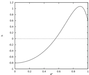
Fig. 3 shows the behavior of h(a∗). The most important feature is that h(a∗) = 0 at a value of a∗≃ 0.555 as seen in the figure. Because a black hole that forms with a value of a∗ > 0.555 will have h(a∗) > 0, ˙a∗ will be negative by Eq. (2.40) and the value of a∗ will decrease as the black hole evaporates, approaching a∗ = 0.555. In contrast, because a black hole that forms with a∗ < 0.555 will have h(a∗) < 0, ˙a∗ will be positive and the value of a∗ will increase towards a∗ = 0.555. Thus, a Kerr black hole emitting massless scalar
-1 -0.8 -0.6 -0.4 -0.2 0 0.2 0.4 0.6 0.8 1 1.2
0 0.2 0.4 0.6 0.8 1
h
a*
Figure 3: The function h(a∗), Eq. (2.41), is plotted as a function of a∗. The point at which h(a∗) = 0 occurs at a∗= 0.555. A hole formed with a∗ on either side of this value will evolve to a state characterized by this value. This figure is taken from Ref. [14].
particles will evolve towards a state with a∗≃ 0.555.
2.3 Evolution of a evaporating Myers-Perry black hole
In this subsection, we discuss the evolution of a five-dimensional rotating black hole emitting scalar particles via the Hawking process for arbitrary initial values of the two rotation parameters a and b. It is found that any such black hole whose initial rotation parameters both nonzero evolves toward an asymptotic stat a/MM P1/2= b/MM P1/2=const.(̸= 0), where this constant is independent of the initial values of a and b.
2.3.1 Myers-Perry solution
The metric of a 5-dimensional rotating black hole is given in the Boyer-Lindquist coordinates as
ds2= − dt2+ (r2+ a21)(dµ21+ µ21dϕ21) + (r2+ a22)(dµ22+ µ22dϕ22)
+ ΠF
Π − µr2dr
2+µr2
ΠF(dt + a1µ
2
1dϕ1+ a2µ22dϕ2)2,
(2.42)
where
F = 1 − a
21µ21
r2+ a21 − a22µ22
r2+ a22, Π = (r
2+ a2
1)(r2+ a22). (2.43)
The metric (2.42) has three parameters. µ gives the black hole mass MM P as MM P = 3π
8Gµ, (2.44)
where G is the five-dimensional gravitational constant. For later convenience, using this parameter, we define a typical scale length as rs:= √µ. The rotation parameters a1 and a2give the angular momenta Jϕ and Jψ as
Jϕ(M P )= 2MM P
3 a1, J
(M P )
ψ =
2MM P
3 a2. (2.45)
The variables µ1 and µ2 obey a constraint
µ21+ µ22= 1. (2.46)
Instead of keeping the symmetric form of the metric (2.42), we solve the constraint (2.46) explicitly. We use the following parametrization
µ1= sin θ, µ2= cos θ, (2.47)
and introduce the following notations
a = a1, b = a2, ϕ = ϕ1, ψ = ϕ2, (2.48) ρ2= r2+ a2cos2θ + b2sin2θ, (2.49)
∆ = (r2+ a2)(r2+ b2) − µr2. (2.50) Then the metric (2.42) takes the form
ds2= − dt2+ (r2+ a2) sin2θdϕ2+ (r2+ b2) cos2θdψ2 + µ
ρ2[dt + a sin2θdϕ + b cos2θdψ]2+r
2ρ2
∆ dr
2+ ρ2dθ2. (2.51)
Three angles take the following values:
0 < ϕ, ψ < 2π, 0 < θ < π/2. (2.52) The metric (2.51) is invariant under the following transformation
a ↔ b, θ ↔ π2 − θ, ϕ ↔ ψ. (2.53)
It possesses 3 Killing vectors, ∂t, ∂ϕ and ∂ψ. The event horizon and the inner horizon of the black hole are located at r+ and r− respectively, where
r2±= 1 2
[µ − a2− b2±√(µ − a2− b2)2− 4a2b2]. (2.54)
The angular velocities Ωa and Ωb are Ωa = a
r2++ a2, Ωb= b
r+2 + b2. (2.55) The temperature and surface gravity of the horizon are
TM P = κM P
2π , κM P =
r2+− r2− 2MM Pr+
. (2.56)
From the condition for the existence of horizon(s), we obtain the condition a + b ≤ rs constraining the angular momenta. In terms of the nondimensional rotation parameter a∗:= a/rs and b∗:= b/rs, the condition becomes
a∗+ b∗≤ 1. (2.57)
Note that we can assume that a ≤ 0 and b ≤ 0 without loss of generality. 2.3.2 Formulation
First, we formulate the time evolution of the Myers-Perry black hole. To quan- tize a massless scalar field Φ, we expand it as Φ = R(r)Θ(θ)eimϕeinψe−iωt. Nomura et al. evaluated the emission rates of the total energy and angular mo- menta by calculating the vacuum expectation value of the energy-momentum tensor of the scalar field (Note that this method to determine the emission rates is different from the method used in Sec. 2.2). Then, the emission rates of the black hole mass MM P and angular momenta Jϕ and Jψ are given by1
−dtd
MM P
Jϕ(M P ) Jψ(M P )
= 1 2π
∑
lmn
∫ ∞ 0
dω Γ
(M P )
lmn(ω)
eω+/TM P − 1
ω m n
. (2.58)
Here, ω+ = ω − mΩϕ− nΩψ, l is the eigenvalue of the angular function Θ(θ) and Γ(M P )lmn (ω) is the greybody factor.
Similarly to Sec. 2.2, we introduce scale invariant rates of change for the mass and angular momenta of an evaporating black hole as
f := −r2sM˙M P ga := −ars
∗
J˙ϕ(M P ), gb:= −rbs
∗
J˙ψ(M P ), (2.59) where the dot ( ˙ ) denotes the derivative with respect to t. In terms of the scale invariant functions f , ga and gb, the time evolution equations for a∗ and b∗are given by
˙a∗ a∗ = −
8 3π
f ha
rs4 ,
˙b∗ b∗ = −
8 3π
f hb
r4s , (2.60)
where the dimensionless functions ha and hb are defined as ha :=3
2 ( ga
f − 1 )
, hb:=3 2
( gb
f − 1 )
. (2.61)
The evolution of a∗and b∗are determined through numerical evaluation of f , ga and gb. In the evolution of Eq. (2.60), a fixed point ha= 0 and hb= 0 plays an important role. Because the mass of an evaporating black hole decreases throughout the Hawking process, f is positive definite. If ha > 0, then a∗ decreases, while if ha < 0, then a∗ increases. Because ha depends not only on a∗but also on b∗, ha= 0 gives a curve in the a∗-b∗ plane.
1The formulas expressed here have different forms from the original ones in Ref. [16] because of the different definitions of the greybody factor.
0.05 0.25 0.45 0.65 0.85 a*
0.05 0.25 0.45 0.65 0.85
b*
0.05 0.25 0.45 0.65 0.85 a*
0.05 0.25 0.45 0.65 0.85
b*
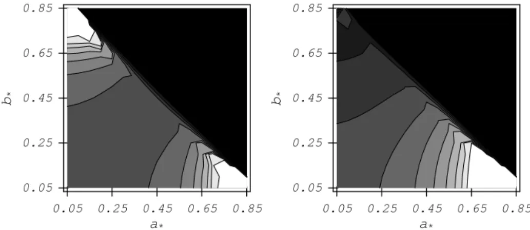
Figure 4: The contours of f (left panel) and ga(right panel) in the a∗-b∗ plane. The black regions correspond to zero, which is forbidden because there is no horizon in this region.. The white regions correspond to the maximums, fmax≃ f (0.85, 0.05) = 4.349 and ga,max ≃ f(0.85, 0.05) = 5.92467. The difference between two contours is fmax/10 in the left panel and ga,max/10 in the right panel. These figures are taken from Ref. [16].
2.3.3 Results
In order to investigate the time evolution of a∗ and b∗, we have to analyze Eq. (2.60). In the following analysis, we use units such that rs = 1. For this purpose, the contour plots of f and ga are depicted in Fig. 4 (gb is obtained by exchanging the axes for a∗ and b∗). In the a∗-b∗ plane, the regions in which a∗+ b∗> 1 is forbidden because there is no horizon (the black regions in Fig. 4). Two white regions in the left panel show that f becomes large, i.e., the emission rate is high. In the right panel, there is only one white region where the angular momentum Jϕ is emitted effectively. If the two rotation parameters are equal (i.e. a∗ = b∗), the emission rates are suppressed even if the black hole is in a maximally rotating state (a∗= b∗= 0.5). In fact, the angular equation for Θ(θ) in this case is exactly the same as that for the Schwarzschild black hole [23]. This is consistent with the result given in Ref. [24].
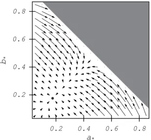
Fig. 5 shows the evolution of a black hole in the a∗-b∗ plane. The vector field ( ˙a∗, ˙b∗) with arrows means how the values of a∗ and b∗ evolve toward the fixed point. The arrows far from the symmetry line of a∗ = b∗ are very large. Then, if the initial value of a∗ (or b∗) is large, a∗ and b∗ approach the same value fast. Near the fixed point (a∗, b∗) = (a(cr)∗ , a(cr)∗ ) ≈ (0.1975, 0.1975), the arrows are very small, which means that the evolution toward the fixed point is slow. We thus find that after reaching a state with a∗ = b∗, a∗ and b∗ eventually evolve together toward the fixed point (a(cr)∗ , a(cr)∗ ). This means that any rotating black hole with two nonzero rotation parameters will evolve toward a final state with the same specific angular momenta, a∗ = b∗ = a(cr)∗ . On the
0.2 0.4 0.6 0.8
a
*0.2 0.4 0.6 0.8
b
*Figure 5: The vector field describes the direction in which a∗ and b∗ evolve, i.e. ( ˙a∗, ˙b∗). For any initial values of a∗ and b∗, the system evolves toward a∗ = b∗ = 0.1975 (the black spot), which is a stable fixed point. The shaded region is forbidden. This figure is taken from Ref. [16].
other hand, for a black hole with only one nonzero rotation parameter, i.e. a ̸= 0 but b = 0 exactly, the stable fixed point is a∗≈ 0.1183, which is determined by the equation ha(a∗, 0) = 0.
In the above analysis, the dynamical system of Eq. (2.60) has one stable attractor, which can be reached through the Hawking evaporation. However, the black hole may evaporate away before this fixed point is reached. This happens if the evaporation time, τM = −M/ ˙M , is longer than the evolution time scale in the a∗-b∗ plane, τa∗ = a∗/| ˙a∗|. Therefore, if the initial mass of the black hole is sufficiently large, the two specific angular momenta will become equal in the Hawking process.
3 Black rings
In this section, we review basic properties of black rings. In addition, we show that for a doubly spinning black ring, there is a limit in which the ring very thin and locally it approaches the geometry of a boosted Kerr black string. This limit was discussed in the more general case of an unbalanced Pomeransky-Sen’kov black ring in Ref. [25].
3.1 An Emparan-Reall black ring
In this subsection, we review a singly spinning black ring. 3.1.1 Emparan-Reall solution
The black ring metic is given by ds2= −F (x)
F (y)
(dt + R√λν(1 + y)dψ)2
+ R
2
(x − y)2 [
− F (x) (
G(y)dψ2+F (y) G(y)dy
2
)
+ F (y)2( dx
2
G(x)+ G(x) F (x)dϕ
2
)] ,
(3.1)
with
F (ξ) = 1 − λξ, G(ξ) = (1 − ξ2)(1 − νξ). (3.2) Note that the form of the solution is not a original one obtained in Ref. [4], but the one revised in Ref. [26]. This solution is characterized by the following three parameters: a length scale R and dimensionless parameters λ and ν.
The range of ν and λ are
0 ≤ ν < λ < 1. (3.3)
In order to avoid a closed timelike curve, we restrict the x range to
−1 ≤ x ≤ 1. (3.4)
The y range is
−∞ < y ≤ −1, λ−1 < y < ∞. (3.5)
|y| = ∞ is a ergoshere, y = 1/ν is a event horizon, y = 1/λ is a singularity inside the event horizon.
In this metric, the surface ”t, y, ψ = const.” corresponds to S2 and x and ϕ are their coordinates. On the other hand, the curve ”t, y, x, ϕ =const.” corre- sponds to S1 and ψ is its coordinate. Therefore, the whole represents a ring- shape S1× S2.
ν parametrize the radius of S2. We recover a very thin black ring as ν → 0. At the opposite limit, the solution represents a very fat black ring as ν → 1.
3.1.2 Conical singularities
The solution generally has conical singularities. We eliminate them because we will consider the balanced black ring(, i.e. the black ring with no conical singularities,) below. Considering an small circle around an axis, we impose the condition for a length of an arc ℓ and an radius r.
2π = ℓ/r (3.6)
First, we obtain the period ∆ϕ of ϕ at x = −1. Using
ℓ =
∫ ∆ϕ 0
√g
ϕϕdϕ = ∆ϕRF (y) (x − y)
√G(x)
F (x), (3.7)
r =
∫ x
−1
√g
xxdx =
∫ x
−1
RF (y) (x − y)
dx
√G(x), (3.8)
the condition for avoiding the conical singularity is 2π = lim
x→−1
ℓ r
=
(lim ∆ϕRF (y)(x−y)) (lim√G(x)F (x)) lim∫−1x RF (y)(x−y)√dx
G(x)
= (
∆ϕ(−1−y)RF (y)) (12√G(−1)F (−1)G
′(−1)F (−1)−G(−1)F′(−1) F2(−1)
)
RF (y) (−1−y)
√ 1 G(−1)
= ∆ϕ G
′(−1)
2√F (−1).
(3.9)
Here we use
x→xlim0
G(x)
F (x)= limx→x0
G′(x)
F′(x). (3.10)
Therefore, the period of ϕ is
∆ϕ = 4π√F (−1) G′(−1) =
2π√1 + λ
1 + ν . (3.11)
As a similar way, one can obtain the period ∆ψ of ψ at y = −1 is
∆ψ = ∆ϕ. (3.12)
The period ∆ϕ′ of ϕ at x = +1 is
∆ϕ′= 4π√F (+1)
|G′(+1)| =
2π√1 − λ
1 − ν . (3.13)
In addition, ∆ϕ′ and ∆ϕ should be identical to each other because they are the periods of the same ϕ:
∆ϕ′ = ∆ϕ. (3.14)
Using λ and ν, we rewrite this condition. λ = 2ν
1 + ν2. (3.15)
3.1.3 Asymptotical flatness
We check asymptotical flatness of the black ring metric at x = y = −1. First, we make the periods of ψ and ϕ 2π with
ψ =˜ 2π
∆ψψ, ϕ =˜ 2π
∆ϕϕ (3.16)
In addition, we define new coordinates ζ and η as ζ = R˜
√−1 − y
(x − y) , η =
R˜√x + 1
(x − y) (3.17)
with
R =˜
√2(1 + λ)
√1 + ν R. (3.18)
Therefore, the metric at x = y = −1
ds2∼ −dt2+ dζ2+ ζ2d ˜ψ2+ dη2+ η2d ˜ϕ2. (3.19) It can be found that the black ring solution is asymptotically flat.
3.1.4 Physical quantities
Using the three parameters ν, λ, R, we show the physical quantities for the Emparan-Reall black ring. Note that ”→” means that we impose the balance condition (3.15).
The mass and angular momentum along S1 are M = 3πR
2
4G
λ(λ + 1) 1 + ν →
3πR2 4G
2ν(1 + ν)
(1 + ν2)2, (3.20) Jψ=πR
3
2G
√λν(1 + λ)5/2 (1 + ν)2 →
πR3 2G
√
2ν2(1 + ν)3
(1 − ν)3(1 + ν2)3. (3.21) Of course, the angular momentum along S2is Jϕ≡ 0. The area and temperature of the horizon are
AH = 8π2R3λ
1/2(1 + λ)(λ − ν)3/2 (1 + ν)2(1 − ν) → 8π
2R3ν2√2(1 − ν)(1 + ν)3
(1 + ν2)3 , (3.22) TH = κ
2π = 1 4πR
1 − ν
√λ(λ − ν) → 1 4πR
1 + ν2
√2
√ 1 − ν
1 + ν, (3.23) where κ is the surface gravity of the horizon.
3.1.5 Non-uniqueness
We focus on the angular momentum normalized by mass j2:= 27π
32G J2 M3 =
(1 + ν)3
8ν . (3.24)
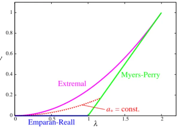
One easily sees that it is infinite at ν = 0, decrease to a minimum value 27/32 at ν = 1/2, and then grows to 1 at ν = 1. This implies that in the range
27 32 ≤ j
2< 1 (3.25)
there exist two black rings with the same value of the spin for fixed mass. This regime of non-uniqueness occurs when the parameter ν takes values in
√5 − 2 ≤ ν < 1. (3.26)
3.1.6 Thin ring limit
There is a limit in which the ring very thin and locally it approaches the geom- etry of a boosted black string. To recover this limit, we focus on a region near the horizon
R → ∞, λ → 0, ν → 0 (3.27)
while keeping Rλ and Rν the following finite value:
Rλ = rHcosh σ, Rν = rHsinh σ. (3.28) Here, we introduced new parameters rH and σ. We also define new coordinates r, θ, and z as
r = −RF (y)y , cos θ = x, z = Rψ. (3.29) The black ring metric (3.1) matches a boosted Schwarzschild black string
ds2= − ¯f (
dt −rHsinh 2σ 2r ¯f dz
)2
+f¯ fdz
2+ 1
fdr
2+ r2dΩ (3.30)
with
f = 1 − rrH, f = 1 −¯ rHcosh
2σ
r . (3.31)
We can find from the metric that rH is a Schwarzschild radius and σ is a boost parameter. Due to the balance condition, the boost parameter takes the constant value, σ = arctan(1/√2).
3.2 A Pomeransky-Sen’kov black ring
In this subsection, we review a doubly spinning black ring. This is the extension of the Emparan-Reall black ring.
3.2.1 Pomeransky-Sen’kov solution
The metric of the Pomeransky-Sen’kov black ring is [10] ds2= −H(y, x)
H(x, y)(dt + Ω)
2−H(y, x)F (x, y)dψ2− 2H(y, x)J(x, y)dψdϕ
+ F (y, x) H(y, x)dϕ
2+ 2R2H(x, y)
(x − y)2(1 − ν)2 ( dx2
G(x)− dy2 G(y)
) ,
(3.32)
where the 1-form Ω is
Ω = −2Rλ
√
(1 + ν)2− λ2 H(y, x)
[(1 − x2) y√νdϕ
+ 1 + y
1 − λ + ν {1 + λ − ν + x2yν (1 − λ − ν) + 2νx (1 − y)} dψ],
(3.33)
and the functions G, H, J and F are
G(x) =(1 − x2) (1 + λx + νx2) , (3.34) H(x, y) =1 + λ2− ν2+ 2λν(1 − x2) y
+ 2xλ(1 − y2ν2) + x2y2ν(1 − λ2− ν2) , (3.35) J(x, y) =2R
2(1 − x2) (1 − y2) λ√ν (x − y) (1 − ν)2
×[1 + λ2− ν2+ 2 (x + y) λν − xyν(1 − λ2− ν2)] ,
(3.36)
F (x, y) = 2R
2
(x − y) (1 − ν)2
× [
G(x)(1 − y2) [{(1 − ν)2− λ2} (1 + ν) + yλ (1 − λ2+ 2ν − 3ν2)] +G(y)[2λ2+ xλ{(1 − ν)2+ λ2} + x2{(1 − ν)2− λ2} (1 + ν)
+ x3λ(1 − λ2− 3ν2+ 2ν3) − x4(1 − ν)ν(−1 + λ2+ ν2) ] ]
. (3.37) Here, we follow the notation of Ref. [10] except that we choose the signature (−, +, +, +, +) for the metric, exchange ϕ and ψ, and use R instead of k. The coordinate ranges are −∞ < t < +∞, 0 < ϕ, ψ < 2π, −1 ≤ x ≤ 1 and
−∞ < y < −1. R is a parameter of dimension of length, which determines the characteristic scale of the S1 radius. λ and ν are dimensionless parameters satisfying 0 ≤ ν < 1 and 2√ν ≤ λ < 1+ν, which determine two nondimensional rotation parameters. The regular event horizon exists at y = yh, where
yh= −λ +
√λ2− 4ν
2ν . (3.38)