RT-Level Design-for-Testability and Expansion of
Functional Test Sequences for Enhanced Defect
Coverage ∗
Alodeep Sanyal† Synopsys Inc. 700 E Middlefield Road Mountain View, CA, USA
Krishnendu Chakrabarty ECE Department
Duke University Durham, NC, USA
Mahmut Yilmaz Advanced Micro Devices Inc.
1 AMD Place Sunnyvale, CA, USA
Hideo Fujiwara School of Information Science Nara Inst. of Science and Technology
Nara, Japan
Abstract— Functional test sequences play an important role in manufacturing test for targeting defects that are not detected by structural test. In practice, functional tests are often derived from existing design-verification test sequences and they suffer from low defect coverage. Therefore, there is a need to increase their effectiveness using design-for-testability (DFT) techniques. We present a non-scan DFT technique at the register-transfer (RT) level that tackles the above problem in three steps. It can be used to increase the defect coverage for scan-based designs by making functional test sequences more effective in native (non-scan) mode. The proposed method selects a small set of control points, and through an efficient branch-and-bound strategy, determines an effective set of truth assignments to these control points (also called test modes). The original functional test is expanded by applying the same functional test sequence once with each selected test mode. Finally, a small set of state elements are chosen as observation points from the transitive fanout cone of the control points based on the number of recorded transitions. The proposed DFT method is evaluated in terms of the unmodeled defect coverage, and we introduce a new surrogate metric, called multi-segment long path sensitization, for the purpose of evaluation. Experimental results for the ITC’99 benchmark circuits, the Open RISC 1200 SoC benchmark, and the Scheduler module of the Illinois Verilog Model (IVM) show that the proposed non-scan DFT technique offers significant potential for ramping up the defect coverage of existing functional test sequences.
I. INTRODUCTION
Nanometer CMOS technologies suffer from high defect rates due to new failure mechanisms. This motivates the need for improved test generation and test application strategies for ensuring high defect coverage. Since structural test alone cannot provide the desired defect coverage [1], functional test is also used in industry to target defects that are not detected by structural test [2]. Therefore, considerable research effort has been devoted to register-transfer (RT)-level fault modeling [3]- [4], test generation [5]-[7], design-for-testability (DFT) [8]- [10],[12]-[14], and test evaluation methods.
A number of methods have been presented in the literature for test generation at RT-level [5]-[7]. However, they usually suffer from low fault coverage due to the lack of gate-level information or due to the poor testability of the design. To
∗This research was supported in part by the Semiconductor Research Corpora- tion under Contract no. 1588. The work of K. Chakrabarty was also supported in part by a Japan Society for Promotion of Science (JSPS) Fellowship.
†The work was done when the author was a visiting research scholar with the Electrical and Computer Engineering Department at Duke University.
increase the testability of large designs and to overcome the difficulty associated with functional test generation, various DFT methods have been proposed. These DFT methods can be classified into two categories: ⟨i⟩ scan-based methods [8]- [9], and ⟨ii⟩ techniques that do not use scan designs [10]- [14]. Although scan-based approaches are easy to implement and offer high controllability and observability of internal state elements, they also suffer from long test application time and problems of overtesting and yield loss [15]-[16]. Moreover, scan-based testing cannot be used to exercise the design in its native functional mode. Non-scan DFT techniques offer an alternative to facilitate functional testing. It can be used to increase the defect coverage for scan-based designs by making functional test sequences more effective in functional (native) mode.
Existing RT-level non-scan DFT methods [10]-[14] focus on increasing the testability of the design to ease subsequent RT-level test generation. However, because of the complexity of functional test generation for large designs, functional test sequences are commonly derived from existing verification test sequences. These test sequences are generated by designers us- ing manual or semi-automated means, and they often suffer from low defect coverage [2]. Therefore, DFT techniques are needed to increase the effectiveness of these functional test sequences. Recently, an RT-level observation point selection method [2] was proposed to enhance defect coverage for existing functional test sequences. A similar DFT technique, shadow scan, was reported by Intel researchers for the recent 8-core Nehalem processor that connects a set of internal state elements in the form of a scan chain and reads the content by scanning them out at the end of the application of functional test [17]. Enhance- ments to scan design proposed for soft-error tolerance [18], [19] may also be used to retrieve error information from internal state elements. However, the observability enhancement through these DFT approaches can provide only limited defect coverage increase, since the quality of the functional test sequence is not being enhanced. It is necessary to improve the controllability of the design as well to achieve high defect coverage during functional test.
In this paper, we address the problem of increasing the defect coverage of a given functional test sequence using the following three-step non-scan DFT technique:
∙ an appropriate selection of a set of control points.
∙ identification of a set of combinations of truth assignments
Paper 21.2 INTERNATIONAL TEST CONFERENCE 1
to these control points (also called test modes) such that the original functional test sequence can be re-applied once with each individual test mode to increase defect coverage.
∙ selection of a small set of observation points to increase the defect coverage even further.
To illustrate the basic idea with the help of an example, let us consider a functional test sequence� with �� patterns. Suppose it takes�� clock cycles to apply the entire functional test sequence. With the proposed approach, if we choose � test modes, it will take �� × � cycles to apply the original functional test sequence once with each individual test mode. Therefore, this notion of “test expansion” leads to an increase in test length. However, note that we do not need to store the expanded functional test �� in the tester. It suffices to store the original functional test sequence in the tester and apply it repeatedly with each individual test mode. The test modes can either be stored on the tester or pre-loaded in the form of on-chip registers. The proposed approach preserves the native functional environment during test, reducing the likelihood of chip over-heating, non-functional state exploration, and yield loss.
One of the basic objectives of the proposed non-scan DFT approach is to sensitize a new set of paths with every single test mode with the aim of increasing the defect coverage. Besides reporting fault coverage for modeled defects, we also evaluate in this work the impact of the proposed DFT method in increasing the unmodeled defect coverage. It is well-known that we cannot accurately evaluate unmodeled defect coverage through simula- tion alone, because this approach relies on models to represent defect behavior. Unmodeled defect coverage can be determined accurately by analyzing silicon data. In this paper, we introduce a new surrogate metric, multi-segment long path sensitization, for the purpose of evaluating unmodeled defect coverage.
The rest of the paper is organized as follows. In Section II, we introduce and formally define the problem. In Section III, we present the proposed approach of control point, test mode and observation point selection. Experimental results are presented in Section IV, followed by conclusions in Section V.
II. PROBLEMFORMULATION
A. Observations and Basic Premise
Unlike existing RT-level DFT approaches that focus on syn- thesizing an easily testable RT-level design with subsequent test generation, we start with an existing functional test sequence.
In this work, our motivation is to target unmodeled defects. Therefore, one of our core objectives is to propagate transi- tions through as many paths in the design as possible. Let us first define the concept of transition for an internal state element. Typically, there is dataflow between registers when an instruction is executed and the dataflow affects the values of registers. Consequently, there are four possible transitions experienced by a given register bit: 0 → 0, 0 → 1, 1 → 0, and1 → 1. After a transition, the final value recorded in a state element can be either correct or faulty (due to a defect). In [20], the authors associated a confidence level (CL) parameter with these four possible transitions that represents the probability that the correct transition occurs for each of these four cases. The CL provides a probabilistic measure of the correct operation of instructions at the RT-level. The confidence level for a
register bit is expressed as a 4-tuple (e.g., ⟨1, 0.998, 0.998, 1⟩ corresponding to the 0 → 0, 0 → 1, 1 → 0, and 1 → 1 transitions respectively). Note that these probabilities can be estimated from failure data or from layout information.
Based on preliminary experiments on ITC’99 bench- marks [4], we made the following two observations, which motivated the subsequent control-point (CP) selection metric: Observation 1:The underlying assumption behind choosing a register bit as a CP and assigning a fixed logic value (0 or 1) to it is that, by doing so, it will sensitize a set of new paths, thereby contributing to the detection of new defects.
Observation 2:A register bit, which exhibits high toggling with the original functional test sequence, should not be considered a CP candidate. Otherwise, we will stabilize a “good” source of transition, adversely affecting the objective of propagating transitions through as many sensitized paths as possible. B. Problem Statement
Let us consider a design with� internal state elements. For an RT-level functional test sequence � with �� instructions, find:
1) a set of� control points (where � ≪ � , i.e., � is much smaller than � );
2) a set of� test modes out of 2� possible truth assignments (� ≪ 2�); and,
3) a set of� observation points (where � ≪ � )
such that the defect coverage is maximized with� control points,
� observation points, and the expanded functional test sequence with� test modes.
III. THEPROPOSEDAPPROACH
A. Control Point Selection
We formally define a selection metric for choosing individual register bits as CPs based on the observations outlined in Section II.
1) Improvement Factor: We observe that, if a given internal state element � records ���0 transitions with the original func- tional test sequence, the testability improvement through this state element depends on:
1) How many more transitions it can record (viz.��− ���0). 2) Its observability (����): the higher the observability of an internal state element, higher is its contribution towards detecting a defect.
3) Weight of the input cone (����): if a state element has a large input cone, it will have a higher chance of being on an error-propagation path. We use a normalized measure for the size of the input cone for individual register bits with respect to the weight of the largest input cone over all bits.
4) Weight of the output cone (����): if a state element has a large output cone, any transition through this state element will have a high likelihood of getting propagated through many downstream paths through its output cone. We use a similar normalized measure with respect to the largest output cone over all internal state elements.
Therefore, the improvement factor �(�) for an individual register bit is expressed as follows:
�(�) = ℘(��−���0)⋅����⋅����⋅���� (1)
Fig. 1. Pseudo-code description of the control point selection procedure
where the probability of transition℘0→1= ℘1→0 = ℘ follows the definition of the confidence level (CL) vector outlined in Section II.
2) Fitness Factor: The fitness factor�(�) for a given register bit � is directly associated with Observation 2 outlined in Section II. The basic idea is that if the total number of transitions recorded by a given register bit � is higher than a user-supplied threshold�∗, the register bit� is eliminated from consideration. Otherwise, a normalized value is assigned to it. We define�(�) as follows:
�(�) =
{0, if ���0≥ �∗ 1 −��
� 0
�∗, otherwise.
(2)
In this work, we use the value��/2 for the threshold �∗, where
�� is the length of the functional test sequence.
3) Selection Metric: The selection metric�� for a given CP candidate� is obtained by combining the fitness factor for the register bit� with the overall improvement achievable through the set of register bits in the transitive fan-out cone of�. The selection metric�� is defined as follows:
�� = �(�)(1 − ∏
�∈� �(�)
�(�)) (3)
where � �(�) represents the set of register bits that are in the transitive fan-out cone of the register bit �. Based on the magnitude of this selection metric, individual CP candidates are sorted in descending order and the top� of them are eventually chosen as CPs. Fig. 1 presents a pseudocode description for the control point selection procedure. The worst-case time complexity of the CP selection procedure is�(�2), where � is the number of internal state elements in a given design. B. Test Mode Selection
After selecting an effective set of � candidates as CPs, our next objective is to identify the specific combinations of truth assignments (also called test modes) for these register bits such that each of these test modes sensitizes a set of previously blocked paths, thereby allowing transitions to propagate through these paths and get recorded at the corresponding destination register bits. Therefore, the increase in transition count in a set of register bits acts as a surrogate metric for increasing defect coverage for a given design.
1) The Bounding Criterion: The exhaustive number of dis- tinct combinations of truth assignments possible with a set of
� selected control points is 2�. It is computationally infeasible
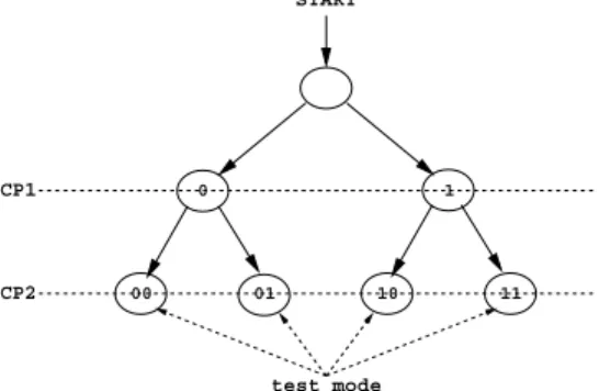
START
CP1
CP2
0 1
00 01 10 11
test mode
Fig. 2. A binary tree visualization of the systematic exploration of the test mode search algorithm
to evaluate the gain in transition in individual register bits as well as for the entire design for each of these test modes and select the best� out of them. It is also impractical to apply all such test modes to expand a given functional test sequence to achieve higher defect coverage. Therefore, an effective strategy is needed to prune out a significant portion of the search space without explicit exploration.
It is easy to visualize the systematic exploration of the search space for test modes in the form of a binary tree (Fig. 2). The rootof this binary tree represents the situation when no control point has been selected. With the selection of the first control point, two new nodes, connected as two children of the root node, are added to the tree, corresponding to the two separate truth assignments to this control point (�� 1). At this point, selection of the second control point (�� 2) and the subsequent truth assignment creates four distinct test modes corresponding to the combinations 00, 01, 10, and 11 respectively for the two selected control points. Therefore, the search space is aptly represented using a complete binary tree with a height� and 2� leaf nodes. Each leaf node represents a distinct truth assignment to the selected control points, also known as a test mode.
To develop a computationally efficient strategy for systematic exploration of the search space, we present the following theorem on a concrete bounding criterion that is applied during the first visit at every single non-leaf node of the binary tree. First we introduce the following definitions.
� �� : total number of transitions recorded in all the register bits in the design after insertion of the �-th control point
� ���� : minimum recorded total transitions over the set of saved � test modes
� �(�) : the fan-out cone of the control point�
�� : total number of patterns in the functional test sequence
���� : total number of transitions recorded at the register bit� with � control points inserted Theorem 1: Suppose a complete set of � test modes has been selected on the basis of total recorded transitions for a given design. A sufficient condition for terminating the mode search after the insertion of � (such that � < �) control points is as follows:
� ��+
�
∑
�=���+1
∑
�∈� �(�)
(�� − ����) ≤ � ���� (4)
If inequality (4) is satisfied, no further increase in transition due
to insertion of additional control points will be able to cross the minimum recorded transitions (� ����) over the saved test modes.
Proof: We prove this theorem using the method of contradic- tion. Suppose after insertion of � control points, the bounding condition is satisfied. We start with the assumption that it is still possible to continue the mode search and eventually record a total number of transitions greater than� ���� over the set of
� saved test modes.
Now, after insertion of� CPs, we are left with �−� remaining candidates from the set of chosen control points whose truth values need to be ascertained. Let us consider the next control point candidate���+1. If a register bit� is in the fan-out cone of control point ���+1, the maximum gain in transition that can occur from the current state is(��− ����), where �� is the length of the original functional test. In this case, we consider the scenario when the given register bit � toggles every single cycle during the functional test.
Therefore, the maximum gain in transition possible over all the fan-out bits of the current control point���+1 is:
��+1= ∑
�∈� �(���+1)
(�� − ����)
In this way, the maximum possible gain����in transition over the fan-out cone of all the remaining control points is:
����=
�
∑
�=���+1
��
During computation of this gain parameter, the register bits that are present in more than one control points’ fan-out cone, are considered only once. We observe that���� is indeed the second term of the bounding condition in the theorem statement, and this gain, when added to the total number of transitions recorded by the register bits in the design at the current state (� ��) with � control points inserted, remains less than the minimum recorded transitions (� ����) over the set of � saved test modes.
Therefore, it is necessary to have additional transitions being recorded at other register bits of the design, which are not in the fanout cone of the remaining� − � control points.
However, this supposition is impossible, because truth assign- ment to a given control point cannot cause any new transition outside its own fanout cone.
This concludes the proof by contradiction. ■ Theorem 1 ensures that the bounding condition never termi- nates a mode search that may eventually find a truth assignment with a higher number of total recorded transitions compared to the existing minimum recorded total transitions over the set of saved� test modes. Therefore, it also guarantees that the set of
� best test modes is preserved at the end of the mode search process.
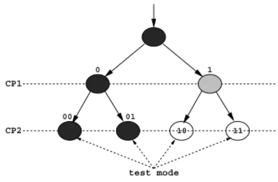
We illustrate Theorem 1 with the following example. Example 1:Let us consider a design with 15 register bits, out of which 2 are chosen as control points. The length of the original functional test sequence is 10. The number of desired test modes as specified by the user is 2. Fig. 3 presents a snapshot of an ongoing mode search process with the control point 1 (�� 1) assigned a logic value 1. The node representing the location
START
CP1
CP2 10 11
test mode 1
00 01
0
Fig. 3. An illustration of the mode search process TABLE I
RECORDEDTRANSITIONS FOR THEFANOUTBITS OFCONTROLPOINT2ON THECURRENTSTATE OF THEMODESEARCH
CP Number of transitions at current state Assignment for the fanout bits of CP2
A B C
CP1=1 5 3 4
of the current mode search is colored gray and the nodes that are already visited by the previous mode searches are colored black. We observe that the mode search process has already saved two test modes (corresponding to the truth assignments 00 and 01). The total number of recorded transitions for these two saved test modes are 78 and 55, respectively, with� ����= 55. With the current mode search, the total number of recorded transitions in the design is 31. At this point, the truth value for the second control point (�� 2) is needed to complete the mode search. There are three register bits �, � and � on the fanout cone of �� 2. The number of recorded transitions in each of them at the current state with �� 1 assigned a logic value 1 are shown in Table I. Therefore, the maximum gain in transition possible for the entire design from this point is: (10 − 5) + (10 − 3) + (10 − 4) = 18. We now evaluate the inequality representing the bounding condition at the current state:31 + 18 = 49 < � ����(= 55). Therefore, we conclude that we can terminate the mode search at this point. ■
2) Mode Search Algorithm: Recursive procedures are typ- ically used to solve problems modeled using binary trees. Starting with the root node, initial recursive calls are made to create/explore the left and the right half of the tree, respectively. In the current context, we adopt the principle of pre-order traversal for implementing the branch-and-bound strategy to systematically explore the entire search space while leveraging the pruning benefit of the bounding criterion. The main steps of the recursive calls to the left sub-tree and the right sub-tree are identical and symmetric in nature. Therefore, we demonstrate the basic steps of the recursive call to the left (right) sub-tree as follows:
STEP 1: Upon selecting a new control point and assigning a truth value of 0 (1), we evaluate the total number of transitions experienced by all the register bits in the entire design thus far, i.e.,� ������.
STEP 2 (a): If the current node is a leaf and the number of leaf nodes visited is less than the number of desired test modes, we do the following:
∙ We store the current leaf as a test mode in the set� � .
∙ We check whether the minimum total transitions (� ����)
recorded over the saved test modes in the� � set is greater than � ������. If so, we update � ���� with � ������ and keep track of the present leaf in the � � set as the min leaf.
STEP 2(b): Otherwise, if the current node is a leaf and the number of leaf nodes visited exceeds the desired number of test modes, then if we observe that the current leaf leads to a higher number of transitions compared to the saved min leaf with� ����, we replace the existing min leaf in the � � set with the current leaf. We then keep track of the next min leaf in the� � set.
STEP 3: If the currently visited node is not a leaf then, based on whether the number of leafs visited so far exceeds the desired number of test modes, we perform one of the following two tasks:
∙ If the number of leafs visited so far already exceeds the desired number of test modes, then we evaluate the bounding condition and decide whether to terminate the current mode search at the current node.
∙ Otherwise, if we have not already saved the desired number of test modes in the � � set, we make recursive calls to the left and right sub-tree of the current node.
3) Time Complexity and Pruning Estimate: The proposed mode search algorithm retains the completeness of the problem. In the worst case, when the bounding criterion is not satisfied for any node in the tree, the algorithm will visit every single node of the tree.
The number of nodes in a complete binary tree with� levels (or control points in this context) is 2�+1− 1. Therefore, the time complexity of the mode search algorithm in the worst case is�(2�). However, through experiments on benchmark circuits, we observe that the proposed algorithm offers a bounding of up to 69%. We also observe that the algorithm offers more pruning for large designs with a high number of control points.
We compute the pruning achieved in the following way. We know the total number of nodes in a complete binary tree with
� levels is 2�+1− 1. Let us assume the number of nodes visited by the current instance of the mode search is � . Therefore, the pruning estimate is:(1 −2�+1�−1) ⋅ 100%. For Example 1 in Section III-B.1, five out of the total of seven nodes were visited, leading to a pruning of 28.57%.
C. Observation Point Selection
After the selection of a small set of control points and test modes to expand a given functional test sequence, our next objective is to select a small set of observation points so that the overall defect coverage improves even further.
We adopt the following simple four-step approach to deter- mine a set of observation points:
1) Identify the set of register bits �� that fall on the transitive fanout cone of the selected control points. 2) Compute the net gain in transition for each of these
register bits � ∈ �� for the expanded functional test
��.
3) Sort the candidate set�� in descending order of net gain in transition.
4) Select the top� candidates from the sorted �� set such that none of them have already been chosen as control point or been directly connected to a primary output.
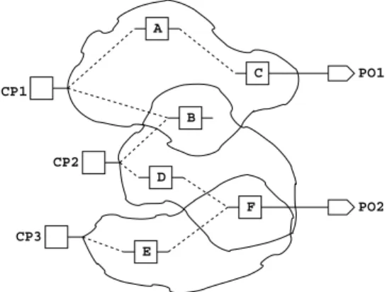
CP1
CP2
CP3
A
C
B
D
E
F PO2
PO1
Fig. 4. An example showing the observation point selection process TABLE II
NETGAIN INTRANSITIONRECORDED BY THEFANOUTBITS OF THE THREECONTROLPOINTS ANDTHEIRRANKS INSORTEDORDER
Register Bit A B C D E F
Transition Gain 23 76 65 39 58 46
Rank Order 6 1 2 5 3 4
The time complexity of the observation point selection algo- rithm is�(�2), where � is the cardinality of the candidate set
�� .
The following example illustrates this approach.
Example 2: Let us consider part of a design shown in Fig. 4 with three control points�� 1, �� 2 and �� 3. Our objective is to select a set of three observation points. The transitive fanout set of �� 1 is {�,�,�}. Similarly, transitive fanout for �� 2 include{�,�,� }, and �� 3 includes {�,� } respectively. The transition gain observed by the fan-out register bits and their relative rank in descending order of transition gain are listed in Table II. From Fig. 4, we observe that the register bits � and� are directly connected to primary outputs. Therefore, the selected observation points are�, �, and �, respectively. ■ D. An Illustrative Example
We explain the operation of the proposed functional DFT method with the aid of the following example.
Example 3: Let us consider an example circuit-under-test (CUT) with six primary inputs (PI) and four primary outputs (PO) (shown in Fig. 5(a)). The functional test sequence � applied to the CUT is of length five (Fig. 5(b)). The proposed DFT method identifies three state elements (namely, �2, �4
and�6) as control points and computes a set of three effetive test modes (out of 23 = 8 possible mode combinations) as presented in Fig. 5(c). Based on the selected control points and test modes, the proposed DFT scheme also identifies three observation points (namely, �7, �9 and �10) following the algorithm presented in Section III-C. The original functional test sequence� is expanded by first applying the test sequence itself without any DFT (by disabling the control points), followed by re-applying the entire test sequence once with each individual test mode. The length of the expanded test sequence becomes 5 × 4 = 20. The expanded functional test sequence is shown in Fig. 5(d). The control points and observation points may be connected to dedicated input and output ports through appropriate multiplexers and demultiplexers. As an alternative, a partial scan chain can be constructed that stitches the control
and observation points together. Individual test modes can be loaded through this scan chain, followed by application of the functional test sequence� , and finally unloading of the response
recorded in the observation points. ■
IV. EXPERIMENTALRESULTS
To evaluate the effectiveness of the proposed RT-level non- scan DFT method, we performed experiments on six represen- tative ITC’99 benchmark circuits [4], and two industry-scale designs, namely, the OpenRISC 1200 processor [21], and the scheduler module of the IVM architecture [22]. Through these experiments, our goal is to show that RT-level control point and observation point insertion, and expansion of functional test sequences by using a set of test modes, improves defect coverage significantly. Our aim is also to demonstrate that it is possible to use the transition characteristics of a design at the RT-level to carry out an efficient branch-and-bound search in finding an effective set of truth assignments for the chosen control points.
A. Experimental Setup
All experiments were performed on a 64-bit Linux server with 4 GB memory. Synopsys Verilog Compiler (VCS) was used to run RT-level Verilog simulation to compute transition characteristics for individual register bits. Design Compiler (DC) from Synopsys was used to synthesize the RT-level Verilog description to a flattened gate-level netlist for each design. The Flextest fault simulator from Mentor Graphics was used to obtain the fault coverage data for the original functional test as well as the resultant test obtained by the proposed test expansion. For the purpose of synthesis, we used the Cadence 180nm technology library. We used Cadence SoC Encounter [23] place-and-route tool to generate delay data (SDF format), parasitic RC data (SPEF format), and the area data for individual benchmarks.
B. Benchmarks Used
We provide a brief description of the benchmarks used to evaluate the proposed DFT approach.
1) ITC’99 Benchmarks: Relevant statistics for the ITC’99 benchmarks are presented in Table III. The functional test sequences for the ITC’99 benchmarks are generated using the RT-level test generation method proposed by Corno et al. [4].
2) OpenRISC 1200 Processor: The OpenRISC 1200 pro- cessor is intended for embedded, portable, and networking applications. It is a 32-bit scaler RISC with 5 stage integer pipeline. It includes the CPU/DSP central block, direct-mapped data cache, direct-mapped instruction cache, data MMU, and instruction MMU based on hash-based TLB. In this work, we only targeted the CPU/DSP unit since it is the central part of the OpenRISC 1200 processor. For OpenRISC 1200, the functional test sequences are obtained from the design-verification tests provided by the developers of the OpenRISC 1200 processor.
3) Scheduler Module of the Illinois Verilog Model: The scheduler is a key component of the IVM architecture [22]. It dynamically schedules instructions. It contains an array of up to 32 instructions waiting to be issued, and can issue six instructions in each clock cycle. The scheduler module has close to 375,000 gates and 8,590 flip-flops. The functional test
R R
R
R
R
R R
R
R
R
1
3 2
4
5
6
7
8
9
10
CP 1 CP 2 CP 3
OP 1 OP 2 OP 3 PI
PO
ModesTest 1 1 0 0 1 0 0 1 1 1 0 1 1 0 0 0 1 1 1 1 1 0 1 0 0 0 1 0 1 1
(b)
0 1 0 1 0 1 1 1 0
1 1 0 1 1 1 1
1 1 1 1
0 0 0 0 1 0 1 1 1 1 1
0 0 0 0
1 1 1 1 0 1 0 0 0 0 0
1 1 1 1
0 0 0 0 0 0 0 0 0
0 0 0 0 0
0 0 0 0 0
1 1 0 0 1 0
1 1 0 0 1 0
1 1 0 0 1 0
1 1 0 0 1 0 0 1 1 1 0 1
0 1 1 1 0 1
0 1 1 1 0 1
0 1 1 1 0 1 1 0 0 0 1 1
1 0 0 0 1 1
1 0 0 0 1 1
1 0 0 0 1 1 1 1 1 0 1 0
1 1 1 0 1 0
1 1 1 0 1 0
1 1 1 0 1 0 0 0 1 0 1 1
0 0 1 0 1 1
0
0 0
0 1
1 0
0 1
1 1
1
(c)
(a)
(d)
Functional Test Sequence
Expanded Test Sequence
Functional Test Sequence Test
Mode
Fig. 5. A depiction of the operation scheme of the functional DFT method: (a) An example circuit-under-test, (b) Original functional test sequence, (c) Test modes, and (d) Expanded functional test sequence
TABLE III
RELEVANTINFORMATION ONITC’99 BENCHMARKS
Benchmark Functionality PI PO Gates FF
b09 Serial to serial converter 3 1 131 28
b10 Voting system 13 6 172 17
b12 One-player game 7 6 1,000 121
b13 Interface to meteo sensors 12 10 309 53 b14 Viper processor (subset) 34 54 3,461 247 b15 80386 processor (subset) 37 70 6,931 447
sequence used for this benchmark is composed of instruction sequences provided by the developers.
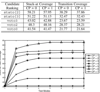
C. Validation of Effectiveness of Control Point Selection To validate the effectiveness of the control point selection method, we choose to use experimental results for the ITC’99 benchmark b10. The original functional test sequence provides 36.89% stuck-at and 20.19% transition fault coverage. Table IV summarizes the fault coverage results when each of the first five control point candidates (identified through the proposed control point selection method) were chosen individually and both the truth assignments (namely, logic 0 and logic 1) were applied separately. We observe that the control point candidates closely follow their ranked order in terms of improving the fault coverage from the base level. Similar experiments with other
TABLE IV
FAULTCOVERAGEPROVIDED BYINDIVIDUALCONTROLPOINT CANDIDATESCHOSEN INRANKORDER FORDESIGN B10
Candidate Stuck-at Coverage Transition Coverage Ranking CP = 0 CP = 1 CP = 0 CP = 1
stato[2] 58.21 57.95 38.29 37.86
stato[3] 51.22 51.13 32.47 32.43
voto3 43.02 42.88 23.67 23.59
voto2 48.3 48.16 28.37 28.21
voto0 41.54 41.47 21.77 21.64
1 2 3 4 5 6 7 8
35 40 45 50 55 60 65 70 75 80 85
Test Modes
Stuck−at Fault Coverage
CP = 1 CP = 2 CP = 3 CP = 4 CP = 5 CP = 6 CP = 7
Fig. 6. Plot showing (a) the improvement in fault coverage upon adding new control points, and (b) the fault coverage saturation after applying a certain number of test modes for the benchmark b13
ITC’99 benchmarks confirmed the observation presented here. D. Selection of Control Points and Test Modes
In the proposed method, the number of control points and test modes are supplied as user parameter. However, for the sake of completeness, we investigate on finding the optimal number of control points and test modes for a given design. We start with the following two hypotheses:
1) For a given number of control points, the fault coverage saturates after the test set is expanded with a certain number of test modes.
2) As we keep on adding control points to a given design, the fault coverage improves up to a certain number of control points, and then the fault coverage may start decreasing. The experimental results for all the ITC’99 benchmarks were in agreement with the above two hypotheses. For the purpose of illustration of the point, let us consider the benchmark b13. The original functional test sequence for the benchmark b13 provides stuck-at fault coverage of 35.9%. The plot in Fig. 6 shows the stuck-at fault coverage for the benchmark b13 with different numbers of control points chosen and test modes applied. We observe that, for a given number of control points, the fault coverage increases initially with the number of test modes applied, and then saturates after a certain number of test modes. Increasing the number of test modes at this point does not improve the fault coverage any further. This is because, with a given set of control points, the expanded test sequence ends up sensitizing close to all possible sets of paths, thereby improving the fault coverage from the base level. Adding a new test mode at this point is unlikely to sensitize any new path.
For the benchmark b13, we also observe that the stuck- at fault coverage with six control points achieves the highest level (the line with the legend “△” in the plot shown in Fig. 6). However, with the next control point chosen from the
sorted candidate list, we observe a drop in the fault coverage (the line with the legend “+” in the plot), suggesting that a suitable number of control points for this design is six. Similar results were obtained with the other five ITC’99 benchmarks. The hypothesis behind this observation is that selection of a state element as a control point essentially blocks transition propagation through it from its fan-in cone. After inserting a certain number of control points, selection of a new control point may open up fewer transition propagation paths on its fan-out cone compared to blocking transition propagation from its fan-in cone resulting in a drop in fault coverage.
E. Defect Coverage Results
We next evaluate the effectiveness of the proposed RT-level non-scan DFT and test expansion approach using several defect coverage metrics. Due to the absence of appropriate RT-level non-scan DFT methods in the existing literature that consider expansion of functional tests, we design the following two baseline methods.
Baseline method 1:First, a set of� control points are randomly chosen from the complete set of register bits for a given design. Next, the chosen register bits are randomly assigned truth values to obtain � unique test modes. Finally, a set of
� observation points are randomly chosen such that none of them have been selected as control points already. This baseline helps us evaluate the effectiveness of the proposed DFT method and test expansion. We choose random selection of control and observation points as a baseline because it is a natural choice from a computational efficiency perspective and has been shown to be effective in other testing problems, e.g., pseudo-random testing to screen a large fraction of all stuck-at faults [24] during production test.
Baseline method 2: The notion of test expansion is a major contribution of this paper. To evaluate the importance of select- ing specific test modes for a given set of control points, we start with the same set of control points as identified by the proposed control point selection method, followed by randomly selecting a set of� unique test modes to expand the original functional test sequence. Finally, we use the proposed observation point selection method to identify a set of� observation points from the transitive fan-out cone of the control points chosen. This baseline can essentially be viewed as a refinement of baseline method 1, particularly tailored to evaluate the importance of selecting a specific set of test modes for a given set of control points.
We compare the relative effectiveness of the proposed method with respect to the above two baseline methods for the six representative ITC’99 benchmarks, the open core 1200 SoC module, and the IVM scheduler module. Table V shows the gate-level stuck-at and transition fault coverage data obtained for the proposed DFT technique and the two baseline methods. In Table VI we present the results for two surrogate fault coverage metrics, namely, BCE+ [25] and the GE score [26]. These fault coverage numbers are attained in a non-scan mode, even though the gate-level design typically uses scan chains for structural test. Since our goal is to enhance testability in the functional (native) mode, we are particularly interested in non-scan fault coverage. In both tables, we provide the number of control (CP) and observation points (OP) selected and test
TABLE V
GATE-LEVELFAULTCOVERAGERESULTS
Benchmark #CP #TM #OP Stuck-at Coverage Transition Coverage
Original DFT-inserted Baseline 1 Baseline 2 Original DFT-inserted Baseline 1 Baseline 2
b09 5 5 5 59.18 94.11 72.95 81.37 47.93 72.83 56.77 62.77
b10 3 2 3 36.89 82.51 52.71 67.89 20.19 60.78 27.98 39.57
b12 3 3 3 50.25 56.12 53.37 54.07 26.67 32.46 29.41 30.07
b13 6 4 6 35.9 85.67 52.38 63.71 23.33 47.95 31.07 34.91
b14 10 2 10 83.95 97.29 88.21 89.45 74.6 84.28 78.67 79.13
b15 10 3 10 9.91 23.92 14.79 17.29 5.35 12.59 9.38 9.97
or1200 cpu 50 4 50 10.33 77.16 42.74 58.64 4.68 43.95 21.87 28.41
IVM Scheduler 80 6 80 21.84 67.94 28.69 39.24 13.08 47.81 22.42 26.79
TABLE VI
GATE-LEVELBCE+ MEASURE ANDGE SCORES
Benchmark #CP #TM #OP BCE+ Measure GE Score
Original DFT-inserted Baseline 1 Baseline 2 Original DFT-inserted Baseline 1 Baseline 2
b09 5 5 5 45.58 84.88 61.23 68.44 121 207 149 163
b10 3 2 3 28.04 71.06 37.52 52.33 132 439 231 317
b12 3 3 3 29.91 33.78 31.79 32.11 889 1,003 947 968
b13 6 4 6 23.11 58.89 45.56 49.07 257 556 351 431
b14 10 2 10 74.52 85.88 79.18 81.74 8,601 9,101 8,778 8,834
b15 10 3 10 4.4 12.23 8.57 9.19 806 2,343 1,671 1,847
or1200 cpu 50 4 50 4.65 47.39 29.47 33.59 1,690 11,323 5,494 7,081
IVM Scheduler 80 6 80 12.58 43.92 20.83 25.91 3,084 14,642 8,971 10,543
modes applied (TM) by the proposed method in Columns 2, 3, and 4, respectively. The column heading Original indicates the case when the original functional test sequence is applied on a given design, whereas the column heading DFT-inserted represents the case when control and observation points have been chosen and the test modes have been applied to expand an original functional test sequence. We performed experiments to find an effective number of control points for each of the ITC’99 benchmarks by inserting one CP at a time and measuring the im- provement in residual fault coverage (mentioned in Section IV- D). For industry-representative designs, a similar experiment was performed in a relatively coarse-grained way. We also kept the number of control and observation points equal for each benchmark for our experiments. The underlying assumption here is to construct a partial scan chain to stitch together the control points and the observation points. Partial scan allows scanning in a specific test mode, followed by applying the functional test sequence and finally, scanning out the captured response from the observation points while scanning in the next test mode. Equal number of control and observation points helps overlapping the scan-in/scan-out operation for subsequent test modes. The baseline methods use the same number of control and observation points and test modes as the proposed method. From Table V and Table VI we observe that the proposed method consistently outperforms the baseline methods. As expected, the baseline method 2 performs better than baseline method 1, since the control and observation points were chosen following the proposed approach as opposed to a random selection. However, for baseline method 2, the test modes were selected by randomly assigning truth values to chosen control points, and therefore, does not show a comparable improvement in fault coverage with respect to the proposed DFT method. We observe particularly impressive results for the industry- representative SoC benchmarks, namely, the or1200 cpu and the IVM Scheduler module. For the or1200 cpu benchmark, we chose 50 control points, 50 observation points, and 4 test modes and observed a rise in stuck-at fault coverage by 7.5X
and transition coverage by 9.4X. For the IVM scheduler module, we used 80 control and observation points and 6 test modes and observed a gain in stuck-at fault coverage by 3.11X and transition fault coverage by 3.66X. Choosing an even larger set of control points is likely to increase the fault coverage even further for these two designs.
From Table V, we also observe that the fault coverage for benchmark b15 does not show significant improvement even after applying the expanded functional test. We attribute this result to the extremely low fault coverage of the original functional test sequence.
F. Evaluation of Unmodeled Defect Coverage
An important goal of functional testing is to increase the unmodeled defect coverage. It is, however, difficult to evaluate the coverage for unmodeled defects. A few surrogate metrics, such as BCE+ [25] and GE Score [26], have been proposed recently to evaluate unmodeled defect coverage. As shown in Table VI, the proposed DFT technique provides higher coverage with respect to BCE+ and GE Score compared to the baseline methods for all the benchmarks.
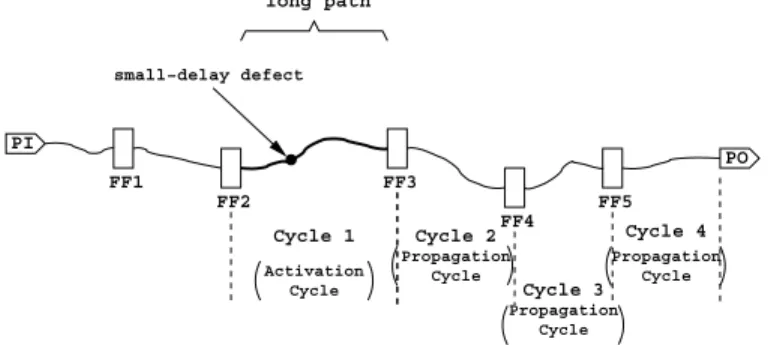
In this paper, we introduce a new surrogate defect-coverage metric, which is particularly suitable for evaluating unmodeled small-delay defect coverage in functional mode. In non-scan (functional) mode, signal-transition propagation includes the following parts:⟨i⟩ a primary input (PI) to a flip-flop, ⟨ii⟩ a flip- flop to a flip-flop, and⟨iii⟩ a flip-flop to a primary output (PO). For the proposed defect-coverage metric, we first identify a set of “long” (i.e., low-slack) paths for the pseudo-combinational model of a given design. A small-delay defect on any of these long paths is assumed to activate a fault that needs to be propagated to an observable output (referred to as the path boundary) through appropriate sensitization to capture an error. If the destination of a given long path is a PO, the error is observed at the end of the current clock cycle (or, in other words, with the clock edge-trigger defining the beginning of the next cycle). In a more general scenario, an error may be captured
FF1 FF3
FF5
PO
FF4 FF2
long path
small−delay defect
PI
Cycle 1 Activation
Cycle
Cycle Propagation
Cycle 4 Propagation
Cycle Cycle 3 Cycle 2
Propagation Cycle
Fig. 7. An example illustrating four-cycle sensitization of a small-delay defect on a long path (four-cycle long path sensitization) in functional mode
TABLE VII
MULTI-SEGMENTLONGPATHSENSITIZATIONRESULTS
Identified Multi-segment
Benchmarks Long Paths Propagation Paths
Original DFT-inserted Original DFT-inserted
b09 7 36 17 457
b10 50 93 73 108
b12 118 94 0 0
b13 24 17 108 143
b14 221,413 194,537 2,402 7,318
b15 1,891 13,669 28 2,658
or1200 cpu 1,546 2,633 17 47
at a flip-flop, and it may need to propagate through a number of flip-flops, each taking one clock cycle, before reaching a PO. Note that the criterion of low slack for a path is required only for the cycle in which the fault is activated. For all subsequent clock cycles needed to propagate the error to a PO, we do not care about the slack of the path, but we only care about path sensitization. The following example illustrates this metric. Example 4:Let us consider an input-to-output path traversing five flip-flops, as shown in Fig. 7. Without loss of generality, we consider any path (PI-to-flop, flop-to-flop, or flop-to-PO) with delay of more than 70% of the clock period to be a long path. In Fig. 7, assume the path segment between FF2 and FF3 (shown in bold) is a long path. For successful detection of any small- delay defect on this path segment, the following two conditions have to be satisfied: ⟨i⟩ the fault should be activated through appropriate PI values and signal propagation to the fault site (possibly through a set of flip-flops in between—the flip-flops FF1 and FF2 in this case), and ⟨ii⟩ the fault effect should be propagated through a sensitized path, possibly traversing through a set of flip-flops (in this case flip-flops FF3, FF4, and FF5), to an observation point. For the example PI-to-PO path shown in Fig. 7, the error due to the delay fault will take four clock cycles, including the fault activation cycle, to reach
the primary output. ■
The proposed defect-coverage metric reports (a) the number of long paths sensitized by a given functional test sequence, and (b) the number of unique sensitized paths (possibly through one or more flip-flops) that originate from the boundary of a long path and terminate at a PO. We call this metric multi- segment long path sensitization (or, in other words, multi-flop long path sensitization). If a given functional test sequence �1
sensitizes a higher number of long paths to an observation point compared to another functional test sequence�2, we expect�1
to be more effective for the detection of small-delay defects.
TABLE VIII
MAXIMUMPATHDELAYOBTAINED THROUGHSTATICTIMINGANALYSIS Benchmark Original DFT-inserted Overhead (%)
b09 1.26 1.39 10.32
b10 1.18 1.32 11.86
b12 3.08 3.08 0.0
b13 1.39 1.48 6.47
b14 14.18 14.80 4.37
b15 27.64 27.87 0.83
or1200 cpu 14.73 15.39 4.48
IVM Scheduler 53.78 53.78 0.0
In Table VII, we report the number of long paths identified, and the number of such paths sensitized to an observation point by the original and the expanded functional test sequences for different benchmarks. As seen in Table VII, the proposed DFT and test expansion method consistently outperforms the original functional test sequence for all the benchmarks. The multi- segment path sensitization metric therefore serves as an useful surrogate metric for the detection of unmodeled small-delay defects.
G. Impact on Timing
It is necessary to investigate the timing impact of any DFT method. We use Synopsys PrimeTime static timing analysis (STA) tool to obtain vector-independent (i.e., static) maximum path delay for a given design and its DFT-inserted counterpart. The STA tool accepts standard delay format (SDF) file and parasitic RC file (SPEF) as input, and analyzes the three different types of combinational logic paths (as mentioned in Section IV-F) to report the path with maximum static delay for each of these three categories. The maximum of these three delay figures is considered the static path delay for a given design, and normally used to determine the clock period for the design. In Table VIII, we summarize the static delay for both the original and the DFT-inserted designs for different benchmarks. We observe that the static delay for a given design increases up to 12% for the ITC’99 benchmarks due to DFT insertion. However, for the two industry-representative designs, the timing overhead is much lower. In fact, we do not observe any timing penalty for the IVM scheduler module, the largest benchmark used in our experiments.
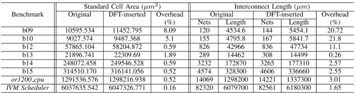
H. Area Overhead
We report the area overhead data for the proposed DFT method as obtained through the Cadence SoC Encounter place- and-route tool [23]. Table IX presents a detailed area overhead data separately for standard cells as well as interconnects. The area overhead is attributed to the two-input multiplexers used to insert control points and buffers used to connect the output of a specific set of state elements directly to primary outputs. From Table IX, we observe that both standard cell area overhead and the interconnect length overhead due to proposed DFT insertion decreases significantly with the increase in original design size. For the industry-representative benchmarks or1200 cpu and the scheduler module of the IVM architecture, both standard cell area and interconnect length overhead become negligible.
V. CONCLUSIONS
We have presented a non-scan DFT technique for testing in functional mode. The proposed method significantly increases