Boosting method via the sparse learner
approach for high-dimensional
gene expression data
DOCTOR OF PHILOSOPHY
Mari Pritchard
Department of Statistical Science
The Graduate University for Advanced Studies
School of 2007
Contents
1 Introduction 6
2 Review of Boosting methods 10
2.1 Notation . . . 10
2.2 Brief history of Boosting . . . 11
2.3 Bagging . . . 12
2.4 Loss function . . . 13
2.5 AdaBoost . . . 14
2.5.1 Algorithm . . . 14
2.5.2 AdaBoost as additive logistic regression model . . . 17
2.5.3 Training error and generalization error . . . 20
2.5.4 Relation to Support Vector Machine . . . 25
2.5.5 Number of iteration and step size to avoid overfitting . . . 29
2.5.6 Relation to Lasso . . . 29
2.6 Boosting variants by different loss function . . . 30
2.6.1 η-Boost . . . 30
2.6.2 Properties of mislabel model . . . 32
2.6.3 LogitBoost . . . 37
2.6.4 SparseL2Boost . . . 38
3 Sparse Learner Boosting 43 3.1 Motivation . . . 43
3.2 Algorithm . . . 43
3.2.1 Trim Overlapping Learners criterion . . . 46
3.3 Complexity of Sparse Learner Boosting . . . 49
3.4 Numerical experiments . . . 51
3.4.1 Cross Validation . . . 52
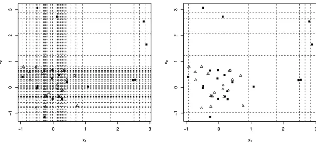
3.4.2 Case 1. Synthetic data with two-dimensional feature vectors . 53 3.4.3 Case 2. Synthetic multivariate data . . . 53
3.5 Real data analysis . . . 56
3.5.1 Microarray technology . . . 56
3.5.2 Pre-processing . . . 58
3.5.3 Boosting method . . . 58
3.5.4 DLDA . . . 59
3.6 Result and discussion . . . 59
3.7 Future work . . . 62
4 Existence of multiple predictive optimum gene sets 63 4.1 Current classification analysis using microarray data . . . 63
4.2 Prediction concordance with small overlap gene sets . . . 64
4.3 Feature selection methods . . . 65
4.4 Feature selection using annotation information . . . 66
4.5 Multiple predictive optimum gene sets . . . 68
4.6 Experiment . . . 68
4.6.1 van’t Veer Method . . . 69
4.7 Result and discussion . . . 70
5 Concluding remarks 76 6 Acknowledgement 77 A Fisher Linear Discriminant Analysis and its variants 79 A.1 Quadratic Discriminant Analysis . . . 80
B Logistic Regression 82
C Derivation of the αt in the AdaBoost algorithm 85
D Derivation of the η-Boost algorithm 86
E Details of Equation (105) 87
F Support Vector Machine 88
Abstract
Gene expression analysis is commonly used to analyze millions of gene ex- pression data points. Challenging in this process has been the development of appropriate statistical methods for high-dimensional data. We propose Sparse Learner Boosting for gene expression data analysis. Boosting is performed to minimize the loss function, although this process can cause overfitting when a large number of variables are present. Ordinary boosting utilizes all of the potential weak learners in a given data set and constructs a decision rule. The fundamental idea of Sparse Learner Boosting is to reduce the complexity of the decision rule by using fewer weak learners than is usually required. This reduction prevents overfitting and improves performance during classification. Numerical studies support this modification for high-dimensional data, such as that obtained from gene expression analysis. We show that the proposed modification improves the performance of ordinary boosting methods. We also review another problem in high-dimensional data. Sparser solutions are desirable from the view point of simple classification modeling and ease of interpretation however there is no unique sparse solution in any single classifi- cation problem. The possible combination of gene sets out of millions of gene expression data is huge. We show the existence of multiple optimum gene sets and consider the possible solutions.
1 Introduction
In the last couple of decades, bioinformatics has showed impressive progress. During the Human Genome Project (Vender et al. (2001)), the speed and cost of reading genome sequence was accelerated that made the end of the project faster than the originally planned. After the project, more species genome were read using the improved technology. More than 1,000 species genomes have finished being read and we can access this genome data on the web site (www.genomesonline.org). Genome information can be utilized in a variety of ways. One technology which uses genome information is microarray technology which measures gene expression levels from collected RNA. Microarray becomes a common technology for its great of interest to observe millions of gene expression behavior.
Microarray has various usages, one of them is in clinical research. Researchers collect gene expression data from patients so that they can examine it with their clin- ical information. Golub et al. (1999) categorized leukemia samples into subclasses using microarray and their clinical outcome information. Bittner et al. (2000) used gene expression data to subgroup melanomas. van’t Veer et al. (2002) published a study to classify metastasis from primary breast cancer patients then their selected genes were used in the first FDA approved microarray diagnosis kit.
The progress of microarray technology has generated a new challenge in statistics and machine learning. Microarray can measure millions of gene expression data in one experiment however still the number of subjects is in the order of hundreds. This extremely unbalanced ratio of dimension p to sample size n makes the application of classic statistical methods challenging without specific modification.
Boosting is introduced by Freund and Schapire (1997) as one of the most powerful methods for machine learning along with Support Vector Machine which is reported by Vapnik (1995). The underlying idea is that many
to build a
learners complicating the classification model. We propose truncating the weak learners candidates while keeping informative weak learners. The motivation for Sparse Learner Boosting is preventing overfitting of high-dimensional data. Early stopping is considered to prevent overfitting and Rosset et al. (2004) explained the relation of early stopping to regularization in boosting. When the size of dimension is large, the learning process proceeds very quickly in a greedy way. This results in complex model which does not have good performance against unknown data. In this case even early stopping does not prevent this behavior. We will show this using synthesized data and real data.
We also review another important problem in this thesis. As a result of tech- nological progress, the possible number of gene expression measurements in one microarray has been rapidly growing, however many genes are not differentially ex- pressed across subjects to any significant degree. These genes are irrelevant for classification purpose, therefore dimension reduction is applied to find differentially expressed genes. Ranking genes by the degree of different expression among class labels is often performed. Some top ranked genes are considered to be useful for clas- sification. As microarray usage for clinical research has become common, researchers in different laboratories have followed a variety of procedures, some similar some dif- ferent. In each case, these researchers expected to see similar genes being selected then used for classification, however overlap was small due to the fact that there is no unique gene set for any given classification problem. Some reasons are considered such as different experiment condition or different patient clinical status. Fan et al. (2006) compared five classification models which used different genes. They showed that four out of five classification methods showed similar prediction performance even though almost no common genes existed across those five methods. We con- sidered multiple optimum gene sets existence in a single data set. We used gene sets
which are not top ranked then compared the classification performance using real data. The result showed the existence of multiple optimum gene sets.
The rest of this thesis is organized as follows. In Section 2, we review Boosting methods, related concepts and variants of Boosting methods. In Section 3 we address the details of Sparse Learner Boosting. In Section 4, we discuss the existence of multiple optimum gene sets. Section 5 is conclusions and remarks.
2 Review of Boosting methods
In this chapter we overview the details of Boosting methods and concepts related to Boosting methods then look at the modification of the original Boosting methods. The main idea of Boosting methods is learning from data sequentially using weak learners which are slightly better than random guesses. Two of the key points of Boosting methods are how to choose the weak classifier to be used for the final classifier and how to combine the selected classifiers. Boosting methods were studied from different view points because of their high performance. We review these different view points. Several weaknesses of Boosting methods and modifications to overcome these flaws have been pointed out. We address some of these weakness and modification in this section.
First we explain the notation. Then we present a brief history of Boosting methods. In section 2.3, we review Bagging which is similar to Boosting methods. In section 2.4, loss functions are mentioned. Then we present the details of AdaBoost and related concepts. Lastly the modifications of the Boosting methods are shown.
2.1 Notation
Before going into detail, we set a notation for the classification procedure. We denote input variables by the symbol X. Output is denoted by Y . We use uppercase letters such as X, Y when referring to the generic aspect of a variable. Let (X, Y ) be a pair of random variables taking values in X × Y where X is a feature space in p-dimension and Y = {−1, +1} is a label set. Observed values are written in lowercase letter. For instance ith value of X is xi. For a given training data set, L = {(xi, yi) : i = (1, . . . , n)}, consisting of n independent, identically distributed pairs having the same distribution as (X, Y ). Let F (x) be a discriminant function associates with a classification rule H(x) which is a function of x into y.
2.2 Brief history of Boosting
The main idea of Boosting is to combine simple ”weak learners” to build a strong learner which has better classification performance than a single learning, this is called ensemble learning. Several researchers reported significant improvements in performance using ensemble learning (Dietterich (2000), Breiman (1996), Breiman (1998), Dietterich and Bakiri (1995)).
Schapire (1990) was the first to provide a polynomial time Boosting algorithm. Drucker et al. (1993) applied the Boosting idea to an OCR task using neural net- works as weak learners. Breiman (1996, 1998) proposed a similar method named bagging and arcing. Schapire and Singer (1999) showed theoretical support for their algorithms in the form of upper bound on generalization error. This theory was developed in the computational learning community based on the concept of PAC learning. Kearns and Valiant (1989) proved that weak learners, each of which per- form slightly better than a guess, can be combined to form a powerful ensemble learning.
AdaBoost (Adaptive Boosting) which is proposed by Freund and Schapire (1997) is the most popular Boosting method. Boosting became common because of high performance. Some researchers stated Boosting did not overfit but some researchers reported Boosting overfit eventually. Boosting is learning from given training data in a greedy way. The algorithm is trying to minimize training error. Therefore if data is very noisy, Boosting learns the noise excessively then causes overfitting. We overview several Boosting methods and their main concepts.
Next we give a brief overview of bagging which has a similar concept to Boosting methods to show why Boosting methods work well.
2.3 Bagging
Breiman (1996, 1998) found that gains in accuracy could be obtained by aggregating predictors built from perturbed version of the training data. Set the training data L = {(xi, yi) : i = (1, . . . , n)}. A bootstrap sample is generated from given training data with replacement. Bootstrap sample is generated as L1, . . . , LB and a classifier Cb is built from each bootstrap sample Lb. Then the final classifier is built from C1, . . . , CB whose output is the class predicted most often by its sub-classifiers. The Bagging algorithm is as follows:
1. For any b = 1, . . . , B
Lb = bootstrap sample from L (1)
Cb(x) = ϕ(x; Lb), (2)
where ϕ is a classifier which returns a predicted label. 2. Final output is
C∗(x) = arg max
y=±1
∑B b=1
I(Cb(x) = y), (3)
where I(·) denotes the indicator function, equaling 1 if the condition in parentheses is true, and otherwise 0.
Bagging updates data sequentially by resampling and then decides the predicted labels by majority votes. On the other Boosting methods use loss function during sequential learning. In the next subsection, we survey a variety of loss functions.
2.4 Loss function
Loss function is a function to measure a penalty incurred by the built model if making a misclassification. There are a variety of loss functions. The common loss functions are denoted by
L(y, F (x)) =
(y − F (x))2 Squared loss exp(−yF (x)) Exponential loss log(1 + exp(−yF (x)) Loglikelihood.
(4)
−1.5 −1.0 −0.5 0.0 0.5 1.0 1.5 2.0
0.00.51.01.52.02.53.0
yF
Loss
−1.5 −1.0 −0.5 0.0 0.5 1.0 1.5 2.0
0.00.51.01.52.02.53.0
yF
Loss
−1.5 −1.0 −0.5 0.0 0.5 1.0 1.5 2.0
0.00.51.01.52.02.53.0
yF
Loss
= Exponential
= Loglikelihood
= Squared Error
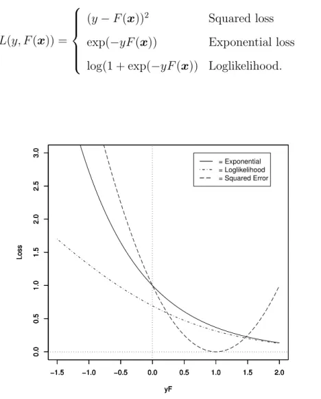
Figure 1: Loss functions. The x-axis is yf and y-axis is loss. Exponential loss, log-likelihood loss and squared loss are drawn.
Figure 1 shows these loss functions as a function of yF . The difference between these loss functions is in the degree of negative penalty. Squared loss is the most
sensitive for the misclassification so it gives a large penalty. The log-likelihood returns a smaller penalty to the misclassified data points than exponential loss. From the view point of optimization, the convex loss function is usually used because of its uniqueness of optimal point. AdaBoost uses the exponential loss function which gives a preferable nature to AdaBoost. We look at the details of AdaBoost algorithm in the next subsection.
2.5 AdaBoost
AdaBoost (Adaptive Boosting) introduced by Freund and Schapire (1997) is the most common Boosting method. AdaBoost builds
of coefficient α and weak learners defined by
F (x) =
∑T t=1
αtft(x). (6)
The coefficient αtand classifiers ftare defined by the following discussion. AdaBoost algorithm is characterized by the minimization of the exponential loss function, which is defined by
Lexp(F ) =
∑n i=1
exp(−yiF (xi)). (7)
Consider an update from F to F + αf each step, the exponential loss function can be written as
Lexp(F + αf ) =
∑n i=1
exp(−yi(F (xi) + αf (xi))) (8)
= ε(f )eα+ (1 − ε(f ))e−α, (9)
where ε(f ) is weighted error rate and defined by
ε(f ) =
∑n i=1
I(yi ̸= f (xi)) exp(−yiF (xi)). (10)
The coefficient α is calculated by
arg min
α∈R
Lexp(F + αf ) = 1 2log
1 − ε(f )
ε(f ) . (11)
The derivation of Equation (11) is written in the Appendix. The optimal value of f on step t is determined by minimizing the weighted error ε(f ). The weight on training example i on step t is denoted by wt(i). Initially, all weights are set equally,
the weak learners are forced to focus on the difficult examples in the training set. The details of algorithm is as follows:
1. Set w1(i) = 1/n and Fo = 0
2. For any t = 1, . . . , T a. Find
ft= arg min
f ∈F
εt(f ) (12)
where
εt(f ) =
∑n i=1
wt(i)I(yi ̸= f (xi)). (13)
b. Calculate
αt= 1 2log
1 − εt(ft)
εt(ft) . (14)
c. Update
wt+1(i) = exp(−αtyift(xi)) Zt
, (15)
where Zt=∑ni=1exp(−αtyift(xi)).
3. The final classifier is given by sgn(F (x)) where F (x) =∑Tt=1αtft(x).
Like Bagging, the AdaBoost algorithm generates a set of classifier and votes them. Beyond this, the main difference between two algorithms is AdaBoost generates the classifier sequentially. On the other hand Bagging can generate them in parallel. On top of the difference, AdaBoost changes the weights of the training samples based
on the previous training result. AdaBoost algorithm increases the weights of exam- ples misclassified by ft and decreases the weights of correctly classified examples. Furthermore AdaBoost algorithm updates the weight of previously selected ftto the worst weight. It can be shown that
εt+1(ft) =
∑n i=1
I(yi ̸= ft(xi))wt+1(i) (16)
=
∑n
i=1I(yi ̸= ft(xi))e(−αtyift(xi))wt(i)
∑n
i=1I(yi ̸= ft(xi))e(αtyift(xi))wt(i) +
∑n
i=1I(yi = ft(xi))e(−αtyift(xi))wt(i)
= 1
2. (17)
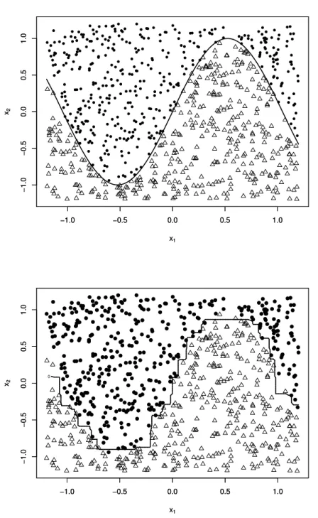
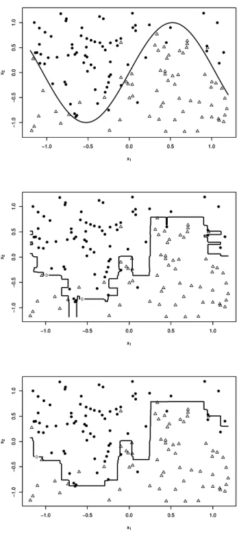
We illustrate a typical example in Figure 2. The data set {(xi, yi) : i = i, . . . , n} was generated as follows. The data x = (x1, x2) was sampled from the uniform distribution U (−1.2, 1.2). The class labels y are defined by
y =
+1 if sin(3x1) ≤ x2
−1 otherwise.
(18)
The left panel in Figure 2 shows the Bayes rule decision boundary. The right panel shows AdaBoost boundary after 100 iterations. We can observe that the AdaBoost boundary is close to the Bayes boundary.
2.5.2 AdaBoost as additive logistic regression model
AdaBoost can be interpreted as a stagewise estimation procedure for fitting an additive logistic regression model. We write the details of logistic regression model in Appendix B. Consider the expectation of the exponential loss function,
J(F ) = E(e−yF (x)), (19)
−1.0 −0.5 0.0 0.5 1.0
−1.0−0.50.00.51.0
x1 x2
−1.0 −0.5 0.0 0.5 1.0
−1.0−0.50.00.51.0
x1 x2
−1.0 −0.5 0.0 0.5 1.0
−1.0−0.50.00.51.0
x1 x2
−1.0 −0.5 0.0 0.5 1.0
−1.0−0.50.00.51.0
x1
x2 0
Figure 2: Typical example: Circles and triangles denote data points with class labels +1 and −1. In the top panel, solid line shows the Bayes rule boundary. In the bottom panel, the solid line shows the AdaBoost boundary after 100 iterations.
where E represents expectation. This can be rewritten as
E(e−yF (x)|x) = P (y = 1|x)e−F (x)+ P (y = −1|x)eF (x). (20)
Minimizing the exponential loss function is equivalent to
∂E(e−yF (x)|x)
∂F (x) = −P (y = 1|x)e−F (x)+ P (y = −1|x)eF (x). (21) Set the derivative to zero,
−P (y = 1|x)e−F (x)+ P (y = −1|x)eF (x) = 0
−P (y = 1|x)e−F (x)+ {1 − P (y = 1|x)}eF (x) = 0
−P (y = 1|x)(e−F (x)+ eF (x)) = −eF (x) P (y = 1|x) = e
F (x)
e−F (x)+ eF (x). (22) In the same way,
P (y = −1|x) = e
−F (x)
e−F (x)+ eF (x). (23)
This is also
F (x) = 1 2log
P (y = +1|x)
P (y = −1|x). (24)
In Equation (24), the left hand term F (x) =∑Tt=1αtft(x), therefore AdaBoost can be considered as an additive logistic regression model.
2.5.3 Training error and generalization error
Freund and Schapire (1997) showed the upper bound of training error. The training error Errtr(F (x)) is
Errtr(F (x)) = 1 n
∑n i=1
I(yi ̸= F (xi)), (25)
which is bounded by
Errtr(F ) ≤ 2T
∏T t=1
√εt(ft)(1 − εt(ft)). (26)
Equation (26) is proved as follows. First we show that
wT +1(i) = 1 n ·
exp(−yiF (x))
∏T t=1Zt
. (27)
It holds that
wt+1(i) = w1(i) ·exp(−α1yif1(xi)) Z1
· · ·exp(−αTyifT(xi)) ZT
(28)
= 1
n ·
exp(−yi∑Tt=1αtft(xi))
∏T t=1Zt
(29)
= 1
n ·
exp(−yiF (x))
∏T t=1Zt
. (30)
The expected exponential loss function can be formed by
L(F ) = 1 n
∑n i=1
exp(−yiF (xi)) (31)
=
∑n i=1
wT +1(i)
∏T t=1
Zt (32)
=
∏T
Zt. (33)
Zt can be rewritten as follows:
Zt =
∑n i=1
wt(i) exp(−αtyift(xi)) (34)
=
∑n i=1
I(yi ̸= f (xi))wt(i)e−α+
∑n i=1
I(yi = f (xi))wt(i)eα (35)
= e(−α)(1 − εt(ft(x))) + e(α)εt(ft(x)) (36)
= 2√εt(ft(x))(1 − εt(ft(x))). (37)
Therefore
L(F ) = 1 n
∑n i=1
exp(−yiF (xi)) = 2T
∏T t=1
√εt(ft(x))(1 − εt(ft(x))). (38)
Since
1 n
∑n i=1
I(yi ̸= F (xi)) ≤ 1 n
∑n i=1
exp(−yiF (xi)), (39)
the upper bound of the training error is
Errtr(F (x)) ≤ 2T
∏T t=1
√εt(ft(x))(1 − εt(ft(x))). (40)
Then this completes the proof.
When εt(ft) ≤ 1/2 − γ ( γ > 0), Equation (40) is
2T
∏T t=1
√εt(ft)(1 − εt(ft)) =
∏T t=1
√1 − 4γt2 (41)
≤ exp (
−2
∑T t=1
γt2 )
. (42)
Then the training error of the combined classifiers decreases exponentially. Freund and Schapire (1997) study the error outside the training data, which is generaliza- tion error. Equation (40) shows that the training error is small; however the interest of classification is in how well the final classifier works against unknown data. The generalization error is the probability of misclassifying a new example, while the test error is the fraction of mistakes on a sample test set, thus generalization er- ror is expected test error. Freund and Schapire (1997) showed how to bound the generalization error of the final classifier in terms of its training error as follows:
P [F (x) ̸= y] + ˜ˆ O
(√T d n
)
, (43)
where ˆP [·] denotes empirical probability on the training sample, n is the size of the sample, d is VC dimension of the base classifier space and T is the number of iterations. VC dimension is a measure of model complexity. We will mention the details of VC dimension later. From the bound of training error suggests that Boosting will overfit if run forever. However some authors observed empirically that Boosting does not cause overfitting, and furthermore, the test error is driven down long after the training error reaches zero.
In response to these empirical findings, Schapire et al. (1998) and Bartlett (1998) gave an alternative analysis in terms of the margins of the training data. Schapire et al. (1998) defined the margin for Boosting methods as follows:
MBoost(x, y) = yF (x)
||α||1
= y
∑T
t=1αtft(x)
||α||1
, (44)
where ||α||1is l1norm for α vector which is α = (α1, . . . , αT). Since the denominator is normalized by the sum of the coefficients αt, the range of the margins is [−1, +1]. The margin is positive if and only if F (x) correctly classifies the example thus the
margin can be read with confidence. They observed that more iterations give a closer value to +1 using separable examples. Schapire et al. (1998) also proved that larger margins on the training set translates into a superior upper bound on the generalization error which is at most
P [Mˆ Boost(x, y) ≤ θ] + ˜O
(√ d nθ2
)
, (45)
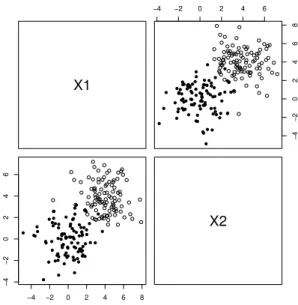
for any θ > 0 with high probability. Schapire et al. (1998) showed the empirical result in his paper. We synthesized a toy example to observe the progress of the margin in accordance with the number of iterations. The plot of the toy example is in Figure 3. Black circles and white circles denote data points with class labels +1 and −1 respectively. The data points with class label +1 follow the normal distribution N ((0, 0), 1.5I). The data points with class labels −1 follow the normal distribution N ((4, 4), 1.5I).
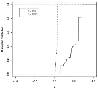
Figure 4 shows the progress of training error and test error. Figure 5 presents the cumulative distribution of margins after 500 and 1000 iterations. Training error reached zero at a very early stage, however the margin becomes larger at 1000 iterations than at 500 iterations.
However the bound is rather weak furthermore when a data sample contains noise, the margin does not approach 1. Grove and Schuurmans (1998) showed an example in which generalization error was not decreased even when the margin goes to 1. The margin theory however is used to explain the connection between AdaBoost and Support Vector Machine. We will review the relation to Support Vector Machine in the next subsection.
X1
−4 −2 0 2 4 6
−4−202468
−4 −2 0 2 4 6 8
−4−20246
X2
Figure 3: Toy example. Black circles and white circles denote data points with class labels +1 and −1 respectively.
0 200 400 600 800 1000
020406080100
Error Rate
step
error rate
0 200 400 600 800 1000
020406080100
Error Rate
step
error rate
0 200 400 600 800 1000
020406080100
step
error rate
Figure 4: Progress of training error and test error. The x-axis is the number of iteration and the y-axis is error. The solid line and dashed line show the progress of training error and test error respectively.
−1.0 −0.5 0.0 0.5 1.0
0.00.20.40.60.81.0
x
Cumulative Distribution
−1.0 −0.5 0.0 0.5 1.0
0.00.20.40.60.81.0
x
Cumulative Distribution
T= 100 T= 1000
Figure 5: The cumulative distribution of margins of the training data after 100 and 1000 times iterations, indicated by dashed line and solid line respectively.
2.5.4 Relation to Support Vector Machine
Support Vector Machine (SVM) is a well known machine learning method as is Boosting method. SVM is introduced by Vapnik (1998). The details of SVM is written in Appendix. Shapire addressed the relationship between AdaBoost and SVM using the margin. The basic concept of SVM is called ’maximum minimum margin’. A data point is viewed as a p-dimensional vector. SVM aims to find a hyperplane which can separate such points. Shapire defined the SVM maxium minimum margin which is
mSVM = min
i
yiF (xi)
||β||2
, (46)
where ||β||2 is the l2 or Euclidean norm of β vector which is β = (β1, . . . , βp). This is similar to the Boosting margin Equation (44). Viewed this way, the connection
between SVM and Boosting method becomes clear. Both methods aim to find a linear combination in a high dimensional space which has a large margin. When described in this manner, SVM and AdaBoost seems to be similar however there are several important differences which Shapire pointed out.
The first one is that different norms can result in very different margins. SVM uses Euclidean norm and Boosting uses l1 norm as the denominator. This difference may not be very significant when one considers low dimensional spaces however in the case of high dimension size, the difference between the norms can result in very large differences in the margin values. The second difference is computational requirements. The computation involved in maximizing the margin is mathematical programming. The difference between the two methods in this regard is that SVM corresponds to quadratic programming, while Boosting method corresponds only to linear programming. The third difference is that different approaches are used to search efficiently in high dimensional space. SVM finds the maximum margin in a high dimensional spaces using kernel trick which is a method to solve a non- linear problem by mapping the original observations into a higher-dimensional space. This makes a linear classification in the higher-dimension equivalent to non-linear classification in the original space. The boosting approach is instead to employ greedy search which adds a weak classifier one by one with re-weighted original data. As kernel trick and greedy search are very different approaches, the resulting learning algorithms can be very different.
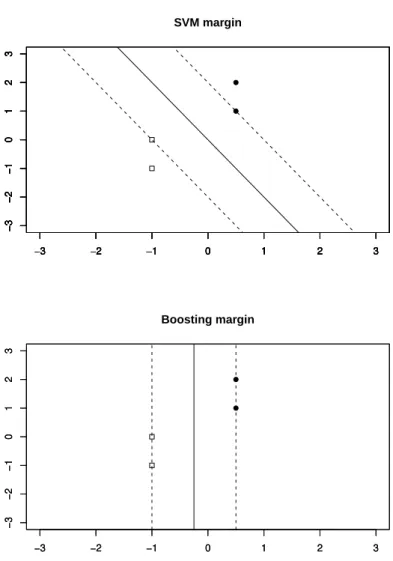
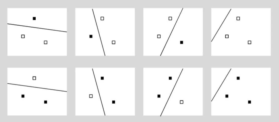
Figure 6 upper panel shows a simple example of separable data in two dimen- sions, with its margin-maximizing separating hyper-plane. The lower panel shows a Boosting margin maximizing separating hyper-plane for the same simple example as the SVM margin.
−3 −2 −1 0 1 2 3
−3−2−10123
−3 −2 −1 0 1 2 3
−3−2−10123
−3 −2 −1 0 1 2 3
−3−2−10123
−3 −2 −1 0 1 2 3
−3−2−10123
−3 −2 −1 0 1 2 3
−3−2−10123
SVM margin
−3 −2 −1 0 1 2 3
−3−2−10123
−3 −2 −1 0 1 2 3
−3−2−10123
Boosting margin
Figure 6: A simple example of two data points in each class. The upper panel shows the SVM margin and the lower panel shows the Boosting margin. The solid line is the boundary.
Rosset et al. (2004) added further interpretation to the Boosting margin relation to the SVM margin. Equation (44) defined the Boosting margin using αtcoordinates which are calculated during Boosting iterations. Rosset et al. (2004) represented the Boosting margin using β and f (x) = x. Boosting discriminant function can be rewritten
F (x) =
∑p j(t)=j
βj(t)fj(x), (47)
where βj(t) =∑j(t)=jαt. Using this notation, minimum of the Boosting margin can be written
mBoost = min
i
yiF (xi)
||β||1 , (48)
where ||β||1 is the l1 norm of β vector which has p dimension. From this repre- sentation, Rosset et al. (2004) showed the relation between mSVM and mBoost as follows:
yF (x)
||β||1 =
yF (x)
||β||2 ·
||β||2
||β||1. (49)
From this representation, we can observe that the Boosting margin will tend to be large if the ratio ||β||2/||β||1 is large. To see this, consider fixing the l1 norm then comparing the l2 norm of two candidates, one with many small components and another with a few large components and many zero components. For example βnon-sparse = (1, 2, 1, 1, 2, 2, 1) and another βsparse = (3, 3, 3, 0, 0, 0, 1). Both l1 norm are the same, 10. Then calculate l2 norm for βnon-sparse and βsparse, which are 16 and 28 respectively. The sparse β vector has a larger l2 norm, hence a larger Boosting margin.
2.5.5 Number of iteration and step size to avoid overfitting
As we described in the previous section, AdaBoost decreases training error expo- nentially but it has a tendency to cause overfitting. Several algorithms are proposed to handle this situation. Grove and Schuurmans (1998) and Jiang (2004) showed that running Boosting forever causes overfitting. Zhang and Yu (2005) proposed that stopping the learning process early prevents overfitting. This is called early stopping. Zhang and Yu (2005) studied the numerical convergence, consistency, and statistical rates of convergence of boosting with early stopping. Using the nu- merical convergence they concluded that the early stopping strategy is shown to be consistent based on iid samples. Besides the number of iterations, step size can cause overfitting as well. Friedman et al. (2000) proposed to fix the step size which is denoted α in Equation (14). The fixed step size Boosting is called ε-boosting. Fried- man et al. (2000) mentioned that fixing the step size to a very small value makes the learning speed slower thus preventing overfitting. This eliminates a favorable statistical property however their empirical results showed a large performance im- provement in regression case. They noted that the change was less significant in zero-one loss.
2.5.6 Relation to Lasso
Rosset et al. (2004) introduced another Boosting methods interpretation. Lasso is tracking a path of approximate solutions to loss function with l1 constrained which is Lasso. Given a convex non-negative loss functions L(·, ·) such as exponential loss or logit loss, consider the 1-dimensional path of optimal solutions to l1 constrained optimization problems over the training data,
β(c) = arg minˆ
∑n
L(yi, βf (xi)). (50)
As c varies, ˆβ(c) traces a 1-dimensional ”optimal curve” through Rp. If an optimal solution for the non-constrained problem exists and has finite l1 norm c0, then β(c) = ˆˆ β(c0) = ˆβ, ∀c > c0. In the case of separable binary class data, there is no finite-norm optimal solution for either exponential loss or logit loss. Then the constrained solutions will always have || ˆβ(c)||1 = c.
A different way of building a solution which has l1 norm c, is to run the ε-boosting algorithm for c/ε iterations. This will give an αc/ε vector which has l1 norm exactly c. For the norm of the geometric representation βc/ε to also be equal to c. Rosset et al. (2004) showed the similarity using real data in their paper.
From the next section, we review the modification of Boosting using different loss functions.
2.6 Boosting variants by different loss function
In the previous section, we addressed the details of AdaBoost. AdaBoost uses the exponential loss function as objective function. As we reviewed in an early section, there are a variety of loss functions. In this section, we present variants of Boosting methods which use different loss functions. We review η-Boost, LogitBoost and SparseL2Boost.
2.6.1 η-Boost
η-Boost is proposed by Takenouchi and Eguchi (2004) as a robust boosting algo- rithm. AdaBoost reportedly can be easily influenced by outliers, which breaks down the performance. η-Boost is defined by the loss function using the following a mix- ture of the exponential loss and naive error loss functions as
Lη(F ) =
∑n i=1
[(1 − η) exp(−yiF (xi)) − ηyiF (xi)]. (51)
where 0 ≤ η ≤ 1. We can derive η-Boost by the sequential minimization of the loss function, Equation (51). See more details Eguchi and Copas (2001). Algorithm is written as follows:
1. Set w∗1(i) = 1/N and F0 = 0
2. For any t = 1, . . . , T a. Find
ft= arg min
f ∈F
ε∗(f ) (52)
where
ε∗t(ft) =
∑n i=1
wt∗(i)I(yi ̸= ft(xi)). (53)
b. Calculate
α∗t = log
√1 − εt(ft) + (ηKt)2 + ηKt
√εt(ft) (54)
where
Kt= (1 − 2ε1(ft)) 2√εt(ft)
((1 − η)Zt
N
)−1
(55)
with
Zt+1 =
∑n i=1
exp(−yiFt(xi)). (56)
c. Update
wt+1∗ (i) = (1 − η) exp(−yiFt(xi)) + η
Zt+1∗ (57)
where
Ft(x) =
∑t m=1
α∗mfm(x) (58)
Zt+1∗ =
∑n i=1
(1 − η) exp(−yiFt(xi)) + η. (59)
3. The discriminant function is sgn(∑Tt=1α∗tft(x)).
The derivations for Equations (53) and (54) are written in the Appendix. Fig (7) shows an example which data has 10 observations were contaminated especially near the boundary. This example addresses that AdaBoost is very sensitive to noise. From the complicated boundary in AdaBoost shows AdaBoost learns from the noise.
2.6.2 Properties of mislabel model
We look at further details of mislabel model. We show some properties of mislabel model which is introduced by Takenouchi et al. (2008). They expand mislabel model to multiclass model. Set G = {1, . . . , K} is finite multiclass labels. Conditional probability of G = g, X = x say p(g|x). Consider mislabel model pζ(g|x) defined by
pζ(g|x) = 1 M (x)
[{
1 −∑
k̸=g
ζk(x) }
p(g|x) +∑
k̸=g
ζk(x)p(k|x) ]
, (60)
−1.0 −0.5 0.0 0.5 1.0
−1.0−0.50.00.51.0
x1 x2
−1.0 −0.5 0.0 0.5 1.0
−1.0−0.50.00.51.0
x1 x2
−1.0 −0.5 0.0 0.5 1.0
−1.0−0.50.00.51.0
x1 x2
−1.0 −0.5 0.0 0.5 1.0
−1.0−0.50.00.51.0
x1 x2
0
0
−1.0 −0.5 0.0 0.5 1.0
−1.0−0.50.00.51.0
x1 x2
−1.0 −0.5 0.0 0.5 1.0
−1.0−0.50.00.51.0
x1 x2
0
Figure 7: Typical example: Circles and triangles denote data points with class labels +1 and −1. In the top panel, solid line shows the Bayes rule boundary. In the center
where M (x) is a normalization constant and ζ(x) is an element which is subset of D, both are defined by
M (x) =
∑g k=1
[{
1 −∑
k̸=g
ζk(x) }
p(g|x) +∑
k̸=g
ζk(x)p(k|x) ]
, (61)
D = {ζ(x) = (ζ1(x), . . . , ζg(x)); 0 ≤∑
k∈G
ζk(x), ζk(x) ≥ 0}. (62)
This shows that ζk(x) is the probability that data is wrongly labeled to class k. The mislabel model which is defined by Equation (60) has the below properties.
Property 1. Posterior probability of pζ(x) obtains the consistency of Bayes rule. M (x) is positive because of the definition thus we only consider inside the bracket then add and subtract ζk(x),
{
1 −∑
k̸=g
ζk(x) }
p(g|x) +∑
k̸=g
ζk(x)p(k|x) (63)
= {
1 −∑
k̸=g
ζk(x) }
p(g|x) − ζk(x) +∑
k̸=g
ζk(x)p(k|x) + ζk(x) (64)
= {
1 −∑
k∈G
ζk(x) }
p(g|x) +∑
k∈G
ζk(x)p(k|x) (65)
= {1 − Kζ(x)} p(g|x) + ζ(x), (66)
which implies that the Bayes rule based on the original posterior p(g|x) is the same as that based on the current posterior pζ(x) for any ζ(x) ∈ D. From this result, for any ζ ∈ D, Fp∗(x) = Fpζ(x).
This can be shown as follows. For any g, k ∈ G and x ∈ X , we observe
pζ(g|x) − pζ(k|x) = {1 − Gζ(x)} {p(g|x) − p(k|x)} (67)
Here 1 − Kζ(x) is positive because ζ(x) > 0, ζ(x) ∈ D and g are invariant.
Property 2. Mislabel model probability pζ(x) follows uniform distribution when mislabel probability ζk(x) follows uniform distribution.
The proof is below. First set
pζ(g|x) = 1 M (x)
[{
1 −∑
k̸=g
ζk(x) }
p(g|x) +∑
k̸=g
ζk(x)p(k|x) ]
.
Set ζk(x) = 1/K then
= 1
M (x) [{
1 −∑
k̸=g
1 K
}
p(g|x) +∑
k̸=g
1
gp(k|x) ]
= 1
M (x) { 1
K
∑
k∈G
p(k|x) }
(68)
= 1
M (x) 1
K. (69)
(70)
From the definition, M = 1 then we could prove that pζ(g|x) = 1/K.
In the next property, we look at the details of error bound. First the error rate is defined by
err(F, p, q) = Probp,q(F (X) ̸= G) (71)
= 1 −∑
g∈G
∫
XgF
p(g|x)q(x)dx, (72)
where XgF = {x|x ∈ X , F (x) = g}.
Then consider a lower bound errbd(p,q) of the error rate under p(g|x)q(x)
errbd(p, q) = err(Fp∗, p, q), (73)
where Fp∗ is Bayes rule. Since Bayes rule is the optimal rule, it is justified to set Bayes rule as the lower bound.
Property 3. For any ζ ∈ D, the relation of the error bound errbd(pζ, q) and errbd(p, q) is
errbd(pζ, q) ≥ errbd(p, q). (74)
From the property 2, we know that a region XFp∗,g coincides with XFpζ ,g. Then
errbd(p, q) = err(Fp∗, p, q)
= 1 −∑
g∈G
∫
XFp ,g∗
p(g|x)q(x)dx
errbd(pζ, q) = err(Fpζ, p, q) (75)
= 1 −∑
g∈G
∫
XFp ,g∗
pζ(g|x)q(x)dx.
Consider
errbd(p, q) − errbd(pζ, q)
= {
1 −∑
g∈G
∫
XF∗
p ,g
p(g|x)q(x)dx }
− {
1 −∑
g∈G
∫
XF∗
p ,g
pζ(g|x)q(x)dx }
(76)
=∑
g∈G
∫
XFp ,g∗
p(g|x)q(x)dx −∑
g∈G
∫
XFp ,g∗
pζ(g|x)q(x)dx (77)
=∑
g∈G
∫
XF∗
p ,g
{p(g|x) − (1 − Kζ(x))p(g|x) + ζ(x)} q(x)dx (78)
=∑
g∈G
∫
XFp ,g∗
{Kζ(x)p(g|x) + ζ(x)} q(x)dx (79)
=∑
g∈G
∫
XF∗
p ,g
{{Kp(g|x) + 1}ζ(x)}q(x)dx (80)
=∑
g∈G
∫
XFp ,g∗
{K{p(g|x) + pU(g|x)}ζ(x)}q(x)dx, (81)
where pU(g|x) is an uniform distribution. We observe for any class label g ∈ G that
x∈ XFp,g∗ ⇒ p(g|x) = max
k∈Gp(k|x) ≥ pU(g). (82)
Therefore errbd(p, q) − errbd(pζ, q) is not negative, which completes the proof.
2.6.3 LogitBoost
We review one more AdaBoost variant, LogitBoost which is introduced by Friedman (2001). LogitBoost relies on the binominal log-likelihood as a loss function, which is a more natural criterion in classification than the exponential criterion underlying the AdaBoost algorithm. Since LogitBoost increases linearly instead of exponen- tially for negative margins. Therefore it can be expected that LogitBoost is more robust in noisy problems. LogitBoost algorithm is written as follows:
1. Set w1(i) = 1/n and F0 = 0 and initial probability estimates p0(xi) = 1/2.
2. For any t = 1, . . . , T a. Calculate
wt(i) = pt−1(xi)(1 − pt−1(xi)), (83) zt−1(i) = yi− pt−1(xi)
wt(i) . (84)
b. Update
Ft(x) =
∑T t=1
1
2ft(x) (85)
pt(xi) = (1 + exp(−2 · Ft(xi)))−1. (86)
We point out that F (x) which LogitBoost algorithm estimates each step is equivalent to estimating of half of the log-odds ratio
F (x) = 1 2log
( p(x) 1 − p(x)
)
. (87)
2.6.4 SparseL2Boost
We review the other Boosting variant aiming for a sparse solution which is named SparseL2Boost proposed by B¨uhlmann and Yu (2006). The title of their paper is Sparse Boosting however they call their algorithm SparseL2Boost in their paper. To avoid confusion with our proposed method and for consistency, we call their method SparseL2Boost in this thesis. SparseL2Boost uses the squared error for the loss function and adds a regularization term. Friedman (2001) proposed L2Boosting which uses the squared loss for Boosting. SparseL2Boost is based on L2Boosting.
Their motivation is similar to ours. In the high dimensional data, there are many irrelevant predictors for classification. Therefore a sparse solution is necessary. The main procedure of L2Boosting simply fits squared error to the current response then uses the residuals from the previous iteration as the new response vector and so on. We first show L2Boosting algorithm then mention SparseL2Boost algorithm. The current response is denoted U = {U1, . . . , Un}.
1. Set F0 = 0.
2. For any t = 1, . . . , T ,
a. calculate residuals Ui = Yi− ˆFt−1(Xi) b. St= arg min
1≤j≤p
∑n
i=1(Ui− γjxij)2
where γj =∑ni=1(Uixij/x2ij) ft(x) = γStx
Ft(x) = Ft−1(x) + νft(x)
where 0 < ν ≤ 1 is a pre-specified step size parameter.
3. Repeat step 2 until some stopping value for the number of iterations is reached.
L2Boosting finds the predictor variable which reduces the residual sum of square most when using least square fitting. They show some variants to choose the best predictor variables in their paper. Here we showed the simplest case. Next we see the sparse L2 Boost.
As L2Boosting is trying to find the predictor variable which minimizes the resid- ual every iteration, B¨uhlmann and Yu (2006) considered L2Boosting is learning in a greedy way. B¨uhlmann and Yu (2006) proposed to choose the predictor variable in the sense of model selection. They construct a function which measures the
complexity of Boosting. First define a hat-operator as follows:
HS : U 7→ (g(xS,U )(x1), . . . , g(xS,U )(xn)), U = (U1, . . . , Un), (88)
where g(xS,U ) = γStx.
Bt= I − (I − νHSt)(I − νHSt−1) · · · (I − νHS1). (89)
The degree of freedom of Boosting is then defined by
trace(Bt) = trace(I − (I − νHSt)(I − νHSt−1) · · · (I − νHS1)) (90)
This is a standard definition for degree of freedom, see Green and Silverman (1994). Therefore the final prediction error criterion proposed by Akaike (1970) can be formed as follows:
∑n i=1
(yi− Ft(xi))2+ τ · trace(Bt). (91)
SparseL2Boost uses Equation (91) as the criterion to move iterations from t − 1 to t. Precisely they set the below objective function so that model complexity can be controlled. The criterion is defined by
T (Y, B) = C(
∑n i=1
(Yi − (BYi))2, trace((B))) (92)
where τ is a parameter for some τ > 0. B¨uhlmann and Yu (2006) mentioned that τ can be decided by cross validation or simply fix 2 or log n such as AIC or BIC. They
also proposed another criterion named gMDL to eliminate the parameter as below
CgM DL(RSS, trace(B)) = log(J) +trace(B)
n log(K), (93)
J = RSS
n − trace(B) (94)
K =
∑n
i=1y2i − RSS
Jtrace(B) (95)
where RSS denotes the residual sum of squares as in Equation (92). Then SparseL2Boost algorithm is as follows:
1. Set F0 = 0
2. For any t = 1, . . . , T Search for the best predictor St= arg min
1≤j≤p
T (Y, B(S))
B⊔(S) = I − (I − HνS⊔)(I − νHS⊔−∞) · · · (I − HνS∞) ft(x) = gSm(X,U )(x)
3. Update
Ft(x) = Ft−1(x) + νft(x)
4. Repeat step 2 and 3 for a large number of iterations T.
5. Estimate the stopping iterations by t∗ = arg min
1≤t≤T
T (Y, trace(B)).
Comparing to the ordinary Boost, SparseL2Boost changed the criterion to choose the best ft(x) using the regularization term. Taking into account the model complexity in the criteria, B¨uhlmann and Yu (2006) considered that the final model could be sparser. Regarding the degree of freedom Hastie (2007) pointed that Equation (91) underestimates of the true degree of freedom using two real data set.
In this section, we overviewed the details of Boosting methods and their modifi- cations. Boosting methods were studied from different view points. AdaBoost can be seen as additive logistic regression. Freund and Schapire (1997) introduced the bound of training error and generalization error. The bound of training gives an idea why training error approaches zero exponentially in terms of number of iterations. Schapire et al. (1998) presented the concept of margin, furthermore they showed the relation to the margin of Support Vector Machine. AdaBoost increases the margin even after training error reaches zero; this may account for the success at reducing generalization error however it was not always true. Rosset et al. (2004) extended the margin theory to the relation to Lasso.
Boosting methods were modified by several approaches. One of them is using different loss function, the second one is using regularization term with loss func- tion. Number of iterations was considered to cause overfitting. Early stopping using cross validation was proposed as a solution. Loss functions and number of itera- tions have been studied for good classification performance however weak classifiers were not studied enough even the complexity of weak learners are in both upper bound of training error and generalization error. Our proposed method focus on the complexity of weak learners which we present further in the next section.
3 Sparse Learner Boosting
In this section, we introduce a new method, Sparse Learner Boosting. Sparse Learner Boosting prevents overfitting by reduction of weak learner candidates. First we mention the motivation of Sparse Learner Boosting. Then we detail the algorithm and examine the model complexity using VC dimension. We show the results of simulation studies using synthesized data and real data.
3.1 Motivation
Boosting methods were studied and improved as we reviewed in the previous section. The key ingredients of Boosting methods are loss function, number of iteration and weak learners. Choosing appropriate of them affects classification performance. A variety of loss functions were studied, early stopping was proposed to prevent over- fitting. On the other hand, choosing weak learners was not studied enough. In gene expression data, size of p is large, hence the candidate weak learners becomes large as well. Using all of them can be superfluous. Therefore we propose a new Boost- ing method trimming the weak learner candidates named Sparse Learner Boosting (Pritchard (2010)).
3.2 Algorithm
We present here the details of Sparse Learner Boosting. Before we describe further details, we define weak learners. We use decision stumps as weak learner candidates, which are defined by
F = {fj(x, a, b) = a · sgn(xj − b) : j ∈ {1, · · · , p}, b ∈ R}, (96)
The idea of Sparse Learner Boosting is to reduce the number of weak learner can- didates. If two class distributions are strongly overlapped, the Boosting algorithm learns from the overlapped samples in a greedy way. The discriminant function becomes complex because of overfitting. Sparse Learner Boosting controls the com- plexity by reducing the number of weak learner candidates using false positive rate and false negative rate. We review the concept of false positive and false negative first then explain our implimentaion.
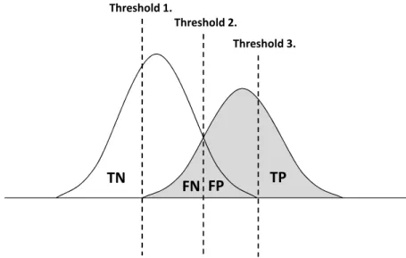
False Positive and False Negative
False positive and false negative are type of errors in which a statistical test wrongly rejects or accepts the null hypothesis. They are often used in diagnostics. In the con- text of a classification problem, considering the cancer diagnostics prediction model, if a patient who does not have cancer is incorrectly diagnosed as having cancer, the consequences may be patient distress plus the need for further investigation. Con- versely, if a patient with cancer is diagnosed as healthy, the result may be premature death due to lack of treatment. In that case, false positive and false negative are considered separately. As an example, let us set that a patient whose label y = +1 has disease and y = −1 has healthy status. If a sick patient is diagnosed as healthy, it is called false negative. If a healthy patient is diagnosed as diseased, it is called false positive. Table 1 shows false positive and false negative in binary classification case. Figure 8 illustrates the relationship between false positive and false negative. Table 1: False Positive and False Negative: Rows express the class label returned by classification rule. Columns express the true labels.
y = +1 y = −1
H(x) = +1 True Positive False Positive H(x) = −1 False Negative True False