本文総合研究大学院大学学術情報リポジトリ甲1588 本文

(1)

Ph.D Thesis

Non-equilibrium Aspects of the Black Hole Thermodynamics

Susumu Okazawa¹

KEK Theory Center, Institute of Particle and Nuclear Studies, High Energy Accelerator Research Organization(KEK)

and

The Graduate University for Advanced Studies (SOKENDAI), Oho 1-1, Tsukuba, Ibaraki 305-0801, Japan

Abstract

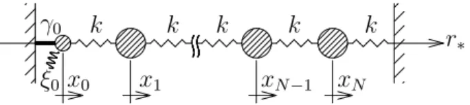
We examine non-equilibrium aspects of the black hole thermodynamics by applying the non-equilibrium fluctuation theorems developed in the statistical physics. In particular, we consider a scalar field in a black hole background. The system of the scalar field behaves stochastically due to the absorption of energy into the black hole and emission of the Hawking radiation from the black hole horizon. We derive the stochastic equations, i.e. the Langevin equation and the Fokker-Planck equations for a scalar field in a black hole background within the ℏ→ 0 limit with the Hawking temperature ℏκ/2π fixed. By applying the fluctuation theorems to these effective equations of motion, we can derive the generalized second law of black hole thermodynamics, a linear response theorem of an energy flow and its nonlinear generalizations as corollaries. We further investigate quantum corrections of the membrane paradigm.

1E-mail address: [email protected]

(2)

1 Introduction

The analogy of the space-time with horizons and thermodynamic systems have been extensively investigated, especially, in the black hole thermodynamics [1]. A black hole behaves like a blackbody with the Hawking temperature TH = ℏκ/2π [2], and energy flowing into the black hole can be identified as the entropy increase of the black hole. Here, κ is the surface gravity at the horizon and the entropy of the black hole SBH is proportional to the area of the event horizon A as SBH = A/4G in the Einstein-Hilbert theory of gravity. The major difference between the black hole thermodynamics and ordinary thermodynamics appears in its origin. The thermal behavior of the black hole thermodynamics is essentially quantum mechanical.

After the discovery of the Hawking radiation, Hawking himself posed a big question which is called “the bleck hole information loss problem” or “the information paradox” [3]. The question is as follows. If matters which have plenty of information collapse into a black hole, it eventually evaporates into space at infinity by the Hawking radiation and becomes gas in thermal equilibrium. It suggests that any initial states will reach a single final state, thermal equilibrium state. If the story is correct, we have to accept the existence of non-unitary evolution in exact sense and give up one of the axioms of quantum mechanics, the unitarity.

There is an apparent weak point in this story, an unequal treatment between matters and gravity. Matters are treated quantum mechanically but gravity is treated in the classical way. We have to find the way of quantization of the black hole to resolve the paradox. Because the question closely relates with a major problem of modern theoretical physics, the quantization of gravity, there were a vast amount of researches which explore the microscopic origin of the black hole. One of the highlights is D-brane construction of extremal black holes in the string theory [4]. The theory tells us that the black hole entropy can be obtained by counting the states of zero modes on D-branes. After that, the AdS/CFT correspondence was founded by Maldacena [5], and the information paradox was investigated in the context of the AdS/CFT correspondence [6].

Although the quantization of the black hole is certainly an important issue, the author draw your attention to incompleteness of our understanding about the ordinary thermodynamics itself. Why can the equilibrium be achieved even though the nature evolves unitarily? This is a simple but cannot be clearly answered question. In other words, we have less knowledge about the dynamics of thermodynamic systems than the equilibrium.

(4)

C The Noise correlation and the Hawking radiation 58

1 Introduction

The analogy of the space-time with horizons and thermodynamic systems have been extensively investigated, especially, in the black hole thermodynamics [1]. A black hole behaves like a blackbody with the Hawking temperature TH = ℏκ/2π [2], and energy flowing into the black hole can be identified as the entropy increase of the black hole. Here, κ is the surface gravity at the horizon and the entropy of the black hole SBH is proportional to the area of the event horizon A as SBH = A/4G in the Einstein-Hilbert theory of gravity. The major difference between the black hole thermodynamics and ordinary thermodynamics appears in its origin. The thermal behavior of the black hole thermodynamics is essentially quantum mechanical.

After the discovery of the Hawking radiation, Hawking himself posed a big question which is called “the bleck hole information loss problem” or “the information paradox” [3]. The question is as follows. If matters which have plenty of information collapse into a black hole, it eventually evaporates into space at infinity by the Hawking radiation and becomes gas in thermal equilibrium. It suggests that any initial states will reach a single final state, thermal equilibrium state. If the story is correct, we have to accept the existence of non-unitary evolution in exact sense and give up one of the axioms of quantum mechanics, the unitarity.

There is an apparent weak point in this story, an unequal treatment between matters and gravity. Matters are treated quantum mechanically but gravity is treated in the classical way. We have to find the way of quantization of the black hole to resolve the paradox. Because the question closely relates with a major problem of modern theoretical physics, the quantization of gravity, there were a vast amount of researches which explore the microscopic origin of the black hole. One of the highlights is D-brane construction of extremal black holes in the string theory [4]. The theory tells us that the black hole entropy can be obtained by counting the states of zero modes on D-branes. After that, the AdS/CFT correspondence was founded by Maldacena [5], and the information paradox was investigated in the context of the AdS/CFT correspondence [6].

Although the quantization of the black hole is certainly an important issue, the author draw your attention to incompleteness of our understanding about the ordinary thermodynamics itself. Why can the equilibrium be achieved even though the nature evolves unitarily? This is a simple but cannot be clearly answered question. In other words, we have less knowledge about the dynamics of thermodynamic systems than the equilibrium.

(5)

The area of the study is called non-equilibrium thermodynamics or non-equilibrium statistical mechanics. We should learn from them to research more about black hole evaporation process.

In thermodynamic systems, entropy is always increasing (or remaining a constant). But if we can measure fluctuations with sufficient precision, which can be realized in mesoscopic systems, there are nonzero probabilities that the entropy of the system de- creases. The fluctuation theorem [7] developed in the non-equilibrium statistical physics relates entropy decreasing probabilities to those of increasing ones. It is a very general theorem that can hold for various non-equilibrium systems including classical Hamilton dynamics in contact with a heat bath, stochastic equations with dissipation and noise, or quantum mechanical systems. The Jarzynski equality [8] relates the work exerted on the system in non-equilibrium situations to equilibrium free energy. It can be derived from the fluctuation theorem, and the second law of thermodynamics is implied from the Jarzynski equality. We use the word implied here because the second law can be derived only if we assume that a system is relaxed to an equilibrium state after a long time.

One of the main purposes of this thesis is to apply the non-equilibrium fluctuation theorem to a scalar field in a black hole background. An application of the fluctuation theorem to a scalar field in a black hole background is straightforward once we obtain a stochastic equation of motion. Because of the thermodynamic behavior of a black hole, a scalar field in a black hole background behaves like a system in contact with a thermal bath. Its effective equation must be described by a stochastic equation with dissipation and quantum noise. The dissipation comes from the classical causal property of the horizon; the black hole horizon absorbs matter and, once they fall in, they cannot come out. The property is the basis of the membrane paradigm of the black hole [9], in which Ohm’s law or the Navior Stokes equations hold on the membrane at the (stretched) horizon. On the other hand, the noise term comes from the Hawking radiation, which is essentially quantum mechanical and, hence, we need to quantize the system in a black hole background in an appropriate way.

The stochastic equation of motion of a string is previously derived in [10, 11] based on physical intuition of the Hawking radiation, or in [12] by using an analogy with the Schwinger-Keldysh formalism in the context of the AdS/CFT correspondence[13]. Our approach is similar to them, but we obtain the effective equation by explicitly integrating fluctuating degrees of freedom. Namely, we introduce infinitely many variables between the horizon and the stretched horizon and consider them as environmental variables. By integrating them, we can show that the variable at the stretched horizon behaves stochastically with a noise term. Though the environmental variables are living outside

(6)

of the horizon, they can encode information in the black hole through choosing the Kruskal vacuum with the regularity condition at the horizon. In this sense, the integration of the environmental variables corresponds to integrating hidden variables in the horizon. The derivation of the Langevin equation is one of our main results. After getting the effective equation of motion, we apply the fluctuation theorem and derive the generalized second law of black hole thermodynamics, or the Green-Kubo formula of linear response and its nonlinear generalizations.

Furthermore, we investigate quantum corrections of the membrane paradigm. The dis- sipative nature of the membrane paradigm is derived by imposing the regularity condition. Our scope is to include the effect of the Hawking radiation as the noise term.

The thesis is organized as follows. In section 2, we briefly review the stochastic approach to thermodynamic systems, the Langevin equation and the Fokker-Planck equation. An important property of the stochastic equation is that it violates the time reversal symmetry which can be measured by an entropy increase in the path integral. In the next section 3, the fluctuation theorem for a stochastic system is reviewed. It relates the entropy increasing and decreasing probabilities. From the fluctuation theorem, the Jarzynski equality is derived. In addition, we explain the fluctuation theorem for a steady state and derivations of nonlinear generalizations of the Green-Kubo formula. In section 4, we derive an effective stochastic equation of a scalar field in a black hole background. In deriving the Langevin equation, the quantum property of the vacuum with the regularity condition at the horizon is very important, which is first explained. We then introduce a set of discretized equations of a scalar field near the black hole horizon, and integrate the variables between the horizon and the stretched horizon. The integration leads to an effective stochastic equation for a variable at the stretched horizon. This has the same spirit as deriving a Langevin equation of a system in contact with a thermal bath [14, 15, 16]. In section 5, we apply the fluctuation theorem to a scalar field in a black hole background. We consider two different situations. In the first case, we put a scalar field and a black hole in a box with an insulating wall. By applying the fluctuation theorem, we can derive a relation connecting entropy decreasing probabilities with increasing ones. From this, the generalized second law of black hole thermodynamics can be derived. In the second case, the wall is assumed to be in contact with a thermal bath of a different temperature which is slightly lower than the Hawking temperature of the black hole. Then there is an energy flow from the black hole to the wall. By applying the steady state fluctuation theorem to it, a linear response theorem of an energy flow to the temperature difference and its non-linear generalizations can be obtained. In section 6, we extend the idea of the membrane paradigm. The equations of the classical membrane paradigm are essentially

(7)

determined by the regularity condition. We further put the effect of the Hawking radiation to it. In the appendix A, we review a derivation of the path integral form of the Fokker-Planck equation. In the appendix B, we review an example of the exact solution of the Fokker-Planck equation. In the appendix C, we will discuss the relation between the noise correlation and the flux of the Hawking radiation.

The contents of this thesis are mainly based on the paper [17].

2 Stochastic Equations of Motion

We first briefly review stochastic approaches to classical statistical systems. In particular, we focus on the path-integral representation (the Onsager-Machlup formalism) of the Fokker-Planck equation and emphasize the role of time-reversal symmetry.

2.1 The Langevin Equation

The Langevin equation is a phenomenological equation of motion of a particle with a friction term and a thermal noise. It is commonly described as

m ˙v = −γv − ^∂V

∂x ^{+ ξ.} ^(2.1)

V (x) is a potential for the particle. γ is a friction coefficient and ξ(t) is a thermal noise (or a random force) which is often assumed to have a Gaussian and white-noise (delta- correlated) distribution

⟨ξ(t)⟩ = 0 , ⟨ξ(t)ξ(t^′)⟩ = 2γT δ(t − t^′^). ^(2.2) The coefficient 2γT is determined to satisfy the equipartition theorem with the temperature T through the fluctuation-dissipation theorem. The noise average ⟨· · · ⟩ can be represented by the following path integral

⟨F (t)⟩ =

∫

DξF (t) exp [

−¹₂

∫

dt1dt2ξ(t1)^δ(t¹^{− t}²⁾ 2γT ^ξ(t²⁾

]

(2.3) with a normalization condition ⟨1⟩ = 1. If necessary, we can easily generalize the noise correlation to an arbitrary colored non-Gaussian noise. An well-known example that can be conveniently described by the Langevin equation is the Brownian motion of a particle or thermal fluctuations of an electric circuit voltage.

(8)

2.2 The Fokker-Planck Equation

From the Langevin equation, we can derive another type of a stochastic equation, the Fokker-Planck equation. It describes a dynamical evolution of the probability distribution P (X, t) of observables X at time t. Here X represents the variables (x, v = ˙x). If the process is Markovian, i.e. the next state is determined only by the present state, the time evolution of P is given by the following Master equation,

∂_t_{P (X, t|X}₀, 0) =

∫

dX^′[w(X^′ _{→ X)P (X}^′_{, t|X}₀, 0) − w(X → X^′)P (X, t|X0, 0)] . (2.4) Here P (X, t|X⁰, 0) is a conditional probability to find an event X(t) = X that has started from the initial value X(0) = X0at t = 0, i.e. P (X, t = 0|X⁰, 0) = δ(X −X⁰^{). w(X}^′ → X) is the transition rate from X^′ to X, which can be related to the Langevin equation in the following way. The first and the second terms of the right hand side of eq.(2.4) describe an incoming and outgoing fluxes of X respectively. The Master equation can be brought into the Kramers-Moyal form as

∂t_{P (X, t|X}0, 0)

= −

∫

dr [w(X → X + r)P (X, t|X⁰, 0) − w(X − r → X)P (X − r, t|X⁰^{, 0)]}

= −

∫

dr_{[1 − e}^−r∂^X] w(X → X + r)P (X, t|X0, 0)

=

∑∞ n=1

(−1)ⁿ n! ^∂

Xn ^[Cn(X)P (X, t|X0^{, 0)] ,} ^(2.5)

where we have defined Cn(X) =

∫

drrⁿw(X → X + r) = lim

∆t→0

1

∆t⟨(X(t + ∆t) − X(t))ⁿ⟩|^X(t)=X^. ^(2.6) In the last line, we have rewritten the n-th moment of the transition rate by a thermal average of an infinitely small variation of the observable X. In this way, we can convert the Langevin equation for dynamical variables to the Fokker-Planck equation for the distribution functions.

Here we show an explicit derivation of the Fokker-Planck equation for the simplest Langevin equation (2.1) as a demonstration. Eq.(2.1) can be considered as a set of first order differential equations for two variables x and v = ˙x. Then the Kramers-Moyal

(9)

coefficients up to the second moments are given by C1(x) = v

C1_{(v) = −}

γ m^{v −}

1 m

∂V

∂x C₂(x) = 0

C2(v) = lim

∆t→0

1

∆t

∫ t+∆t t

dt1

∫ t+∆t t

dt2_{⟨ ˙v(t}1) ˙v(t2_)⟩|x(t)=x

= lim

∆t→0

( 1

∆t

∫ t+∆t t

dt1

2γT

m² ^{+ O(∆t)} )

= ^2γT

m² ^. ^(2.7)

Higher order coefficients vanish in the ∆t → 0 limit. Now we get the Fokker-Planck equation corresponding to the Langevin equation (2.1);

∂tP (x, v, t|x⁰^{, v}⁰^{, 0) = ∂}^x(−vP ) + ∂^v^{[( γ}_m^{v +}_m¹ ^∂V_∂x )

P ]

+ ∂²_v^{( γT} m²^P

)

. (2.8) This Fokker-Planck equation has a simple solution

P^st _{∝ e}⁻^T¹⁽¹²^mv²^{+V (x)}). (2.9)

Note that both of −v∂^x^{P +}m¹

∂V

∂x^∂^v^{P and ∂}^v

[_γ

m^{vP +} γT

m²^∂^v^P] cancel for P^st. It is the well- known Maxwell-Boltzmann distribution for a system in the equilibrium with temperature T , and satisfies the stationarity condition ∂tP^st = 0. The solution satisfies the equilibrium condition, stronger than the stationarity condition.

Here we have used the words “stationary” and “equilibrium” in the following sense. Stationary distributions are solutions to the Fokker-Planck equation satisfying ∂tP = 0. Equilibrium distributions are also stationary but satisfy a stronger condition which is called the detailed balance condition. The most direct definition of the detailed balance condition is given in the language of the Master equation. Due to the definition of stationarity, P^st satisfies ∫ dX^′[w(X^′ _{→ X)P}^st(X^′) − w(X → X^′^)P^st(X)] = 0 for arbitrary X. On the other hand, the detailed balance condition is defined as

∀X, X^′^{, w(X}^′ → X)P^st^(X^′) − w(X → X^′^)P^st^{(X) = 0.} ^(2.10) To satisfy this condition, the system must have the microscopic time reversal symmetry and can not have a specific arrow of time. In other words, there is no entropy production. In a stationary but non-equilibrium configuration, there is a flow of current in a configuration space (x, v).

(10)

The solution of the Fokker-Planck equation can be represented in a path integral form as

P (x, t|x⁰^{, 0) =}

∫ x(t)=x x(0)=x0

Dx exp [

−_4γT¹

∫ t 0

dt^′(m¨x + γ ˙x + ^∂V_∂x⁾² ]

(2.11) Its derivation is explained in the appendix A. The “Lagrangian” L = _4γT¹ (m¨x + γ ˙x +^∂V_∂x)² is called the Onsager-Machlup function [18]. A variation of the Onsager-Machlup function gives the most probable path in the stochastic processes. Apparently, since we have L ≥ 0, the paths satisfying L = 0 are most favored if exist.

The Onsager-Machlup function can be divided into two parts, 1

4γT ^{(m¨x +}

∂V

∂x

)2

+ ^γ 4T ^˙x

2 _(2.12)

which preserves time reversal symmetry, and the remaining is a violating term,

− ¹

2T ^˙x^{(m¨x +}

∂V

∂x^{) .} ^(2.13)

The latter plays an important role to prove the fluctuation theorem in the next section.

3 Non-equilibrium Identities

The stochastic equations such as the Langevin or the Fokker-Planck equations describe how a system is dynamically relaxed to a stationary or an equilibrium state. Furthermore we can calculate transition amplitudes of a system to one state to another. By using the method reviewed in the previous section, we can calculate a ratio of an entropy decreasing probability to an entropy increasing probability. Since the latter probabilities have always much bigger values, the entropy is always increasing after we take a stochastic average.

In this section we review a derivation of the fluctuation theorem and the Jarzynski equality from the stochastic equations.

3.1 The Fluctuation Theorem

The fluctuation theorem was first discovered in numerical simulations [7] and gives the ratio of probabilities of an entropy increasing process to that of a decreasing one. The proof of the fluctuation theorem is given for various systems including classical Hamiltonian dynamics [19], stochastic Langevin dynamics [20] and quantum mechanical evolutions [21, 22]. The Jarzynski equality [8] is a relation between non-equilibrium work and equilibrium free energy difference, and both of them are remarkable discoveries in the recent

(11)

developments of non-equilibrium statistical physics. In this thesis, we concentrate on a system that the evolution is described by the Fokker-Planck equation such as eq.(2.8). The fluctuation theorems can be simply derived and the meaning of entropy production (or the violation of time-reversal symmetry) is clear.

We consider a stochastic system described by the Langevin equation (2.1) or the Fokker-Planck equation (2.8). In order to study a dynamical evolution, we introduce an externally controlled parameter λ^F_t in the potential V (x; λ^F_t). By changing the external parameter λ^F_t as a function of t, the corresponding stable state changes accordingly with time. For later convenience, we call the process of changing the external parameter with λ^F_t as the “forward protocol”. For example, we may set the minimum position of a harmonic potential as the externally controlled parameter;

V (x; λ^F_t) = ¹

2^{k(x − λ}

F

t⁾²^, ^(3.1)

if the position moves linearly with time t, the parameter is given by λ^F_t = v0t. We can also take different protocols e.g. oscillatory or pulse-like etc.

From the path integral representation of the transition rate (2.11), a probability that a sequence of configurations Γτ = {x(t), t ∈ [0, τ]|x(0) = xⁱⁿⁱ, x(τ ) = xfin} is realized during the time interval t ∈ [0, τ] is given by

P^F[Γ_τ_|x_ini_{] ∝ exp} [

−_4γT¹

∫

Γτ

dt⁽m¨x + γ ˙x + ^{∂V (x;λ}_∂x ^F^t⁾⁾² ]

. (3.2)

The trajectory Γτ represents a sequence of configurations in the forward protocol λ^F_t with the initial configuration x(0) = xini.

We now define a time reversal of the forward protocol λ^F_t, and call it the “reversed protocol” λ^R_t _{≡ λ}^F_{τ −t}. We consider a probability P^R[Γ^∗_τ_|xfin] that the system experiences a reversed trajectory Γ^∗_τ _{= {x}^∗(t) ≡ x(τ −t), t ∈ [0, τ]|x^∗^{(0) = x}^fin^{, x}^∗^{(τ ) = x}ⁱⁿⁱ} in the time- reversed protocol λ^R_t. The reversed trajectory has the initial value x^∗(0) = xfin = x(τ ),

˙x^∗(0) = − ˙x(τ). If the system has time-reversal symmetry, the probability should be the same as the probability P^F[Γτ_|xini]. But since the stochastic equation violates the symmetry, they will be different. The reversed propability P^R[Γ^∗_τ_|xfin] is similarly given by

P^R[Γ^∗_τ_|xfin_{] ∝ exp}

[

−_4γT¹

∫

Γ^∗τ

dt⁽m¨x + γ ˙x + ^{∂V (x;λ}_∂x^R^t⁾⁾² ]

= exp [

−_4γT¹

∫

Γτ

dt^′⁽m¨_{x − γ ˙x +}^{∂V (x;λ}_∂x ^F^t′⁾⁾² ]

. (3.3)

(12)

In the last line, we change a variable from t to t^′ = τ − t. This change causes a flip of the sign of ˙x. The ratio of P^F and P^R now becomes

P^F[Γτ_|xini]

P^R[Γ^∗_τ_|xfin] ^{= exp} [

−_T¹

∫

Γτ

dt ˙x⁽m¨x +^{∂V (x;λ}_∂x^F^t⁾⁾ ]

. (3.4)

This gives a key property to prove the fluctuation theorem. Time-reversal symmetric terms are canceled between P^F and P^R, and the ratio is given by the entropy production S of the stochastic process.˙

We further need to sum over the initial configurations, xini and xfin respectively for the forward and the reversed protocols, with appropriate statistical weights. Here we assume that the external parameter is kept fixed at the initial value of each protocol before t = 0. Hence the system is in the equilibrium. We therefore multiply P^F or P^R by the Boltzmann weight P^eq(xini) or P^eq(xfin). The ratio of the Boltzmann weights for the initial configurations is given by

P^eq(x_ini) P^eq(xfin) ⁼

Z(λ^F_τ) Z(λ^F₀)^exp

[

−_T¹ ^{( 1}₂^{m( ˙x}²ini− ˙x²fin^{) + V (x}ini; λ^F₀_{) − V (x}fin; λ^F_τ) )]

= exp^{[ 1} T

∫

Γτ

dt (

m ˙x¨x + ˙x^{∂V (x; λ}

Ft⁾

∂x ^{+ ˙λ}

F t

∂V (x; λ^F_t )

∂λ^F_t )

−^∆F T

]

, (3.5) where ∆F is the difference of the free energy F (λ) = −T log Z(λ) of equilibrium states at λ = λ^F₀ and λ = λ^F_τ,

∆F = F (λ^F_τ_{) − F (λ}^F₀). (3.6)

Combining the two ratios eq.(3.4) and eq.(3.5), we get the following relation, P^F[Γ_τ_|x_ini]P^eq(x_ini)

P^R[Γ^∗_τ_|xfin]P^eq(xfin) ^{= exp (R[Γ}^τ^{]) .} ^(3.7) We have defined R[Γτ] and W [Γτ] as

R[Γτ_{] ≡}

1 T

∫

Γτ

dt ˙λ^F_t ^{∂V (x; λ}

Ft ⁾

∂λ^F_t ⁻

∆F

T ^{≡ W [Γ}^τ^{] −}

∆F

T ^(3.8)

which measures the entropy production in the trajectory Γ_τ and the work exerted on the system.

As a simple example, for the potential V (x; λ^F_t ) = k(x − v0^t)²/2, we have R[Γτ_{] = −}

1 T

∫

Γτ

dtv0_{k(x(t) − v}0t). (3.9)

(13)

(a) v0

ξ F

x

(b) v0

ξ F

x Figure 1: (a) A schematic illustration of motion of a particle in the potential V (x; λ^F_t ) =

1

2^{k(x − v}⁰^t)

2. This picture shows a natural configuration with (x(t) − v⁰t) < 0. It gives a positive value of R[Γτ]. (b) A noise ξ rarely pushes a particle to the opposite side beyond the minimum point x(t) = v0t. Since (x(t) − v⁰t) > 0, it gives a negative value of R[Γτ]

The term, velocity times force, gives a work exerted on the system. If we neglected the fluctuation of the particle, x(t) − v⁰t would always have a negative sign, and R[Γτ] would always increase. It is consistent with a naive picture. However in a mesoscopic system, fluctuations can grow larger and x(t) − v⁰t can have a positive sign. Then the particle overshoots the minimum point ∂xV = 0 to the positive side and R[Γτ] becomes negative. Such a negative value of R[Γτ] indicates that the system exerts work onto outside and it gives a negative entropy production.

From the equation (3.7), by integrating all paths of the configurations, we can derive the fluctuation theorem in the final form as

ρ^F(Rτ_{) ≡}

∫

DxP^F^[Γ^τ|xⁱⁿⁱ^]P^eq^(xⁱⁿⁱ^)δ(R^τ − R[Γ^τ^])

=

∫

DxP^R^[Γ^∗τ|x^fin^]P^eq^(x^fin^)e^R[Γ^τ^]^δ(R^τ − R[Γ^τ^])

= e^R^τ

∫

DxP^R^[Γ^∗τ|x^fin^]P^eq^(x^fin^)δ(R^τ ^{+ R[Γ}^∗τ^])

= e^R^τρ^R_(−Rτ). (3.10)

The first line is the definition of ρ^F(Rτ), i.e. the probability to get the entropy production Rτ within the interval [0, τ ]. We use the relation (3.7) in the second line. In the third equality the relation R[Γ^∗_τ_{] = −R[Γ}τ] is used. Since the quantity Rτ measures the entropy production in the interval, we see that entropy decreasing probabilities are related to increasing ones. They are exponentially suppressed, but exist with nonzero probabilities.

(14)

3.2 The Jarzynski Equality

By integrating the fluctuation theorem over the entropy production, we can construct an equality, so called the Jarzynski equality [23].

∫ _∞

−∞

dRτρ^F(Rτ)e^−R^τ =

∫ _∞

−∞

dRτρ^R_(−Rτ)

⇒ ⟨e^−R^τ⟩ = 1. ^(3.11)

We have defined the average as

⟨F (R^τ)⟩ =

∫ _∞

−∞

dRτρ^F(Rτ)F (Rτ) =

∫

DxP^F^[Γ^τ|xⁱⁿⁱ^]P^eq^(xⁱⁿⁱ^{)F (R[Γ}^τ^]). ^(3.12) The Jarzynski equality (3.11) states that the weighted sum of e^−R^τ over all possible non- equilibrium processes with an externally controlled potential gives an unity. In terms of the work exerted on the system W [Γτ] and the free energy difference, we can relate an average work done in non-equilibrium processes to the equilibrium free energy difference [8] as

⟨e⁻^W^T⟩ = e⁻^∆F^T ^. ^(3.13)

From this equation, by using the Jensen inequality ⟨e^x⟩ ≥ e^⟨x⟩, we get an inequality;

⟨W ⟩ − ∆F ≥ 0. ^(3.14)

This indicates the second law of thermodynamics. The Jarzynski equality simply states that there must exist microscopic processes with large negative entropy productions to satisfy the equality, and the probability is characterized by the equilibrium quantity of the free energy difference.

Some comments are in order. First, the notion of entropy is usually defined for a thermal system after taking an average. It may be appropriate to use a word, the entropy function, instead of the entropy for each microscopic configuration. The second comment is that the above derivation of the second law is justified if the system can relax to an equilibrium state with the fixed external parameter after a long time interval. Since the system is in contact with a large heat bath with temperature T , the relaxed state coin- cides with the equilibrium state at the temperature. If this is the case, the second law of thermodynamics is derived from the Jarzynski equality. In the present proof of the fluctuation theorem, we have used the stochastic approach and the system explicitly violates the time-reversal symmetry. Then such a relaxation can occur. But if we start from the

(15)

original unitary quantum mechanical evolution, the system cannot be thermalized in an exact sense. In applying the fluctuation theorem to the information paradox of the black hole, such considerations are inevitable. The clear understanding about the thermaliza- tion problem of reversible classical systems or quantum mechanical systems has not been obtained as far as the author knows.

An alternative expression of the fluctuation theorem is obtained by using the generating function. We define the generating function for Rτ as

Z^F(ατ) = ln (∫ _∞

−∞

dRτe^iα^τ^R^τρ^F(Rτ) )

. (3.15)

Derivatives of Z^F(α_τ) give connected correlators of the entropy production R_τ in a situ- ation of the forwardly varying parameter. One easily gets the following relation between Z^F(α_τ) and Z^R(α_τ) from the fluctuation theorem as

Z^F(ατ) = ln (∫ _∞

−∞

dRτe^iα^τ^R^τe^R^τρ^R_(−Rτ) )

= ln (∫ _∞

−∞

dxe^ix(i−α^τ⁾ρ^R(x) )

= Z^R_{(i − α}τ). (3.16)

We have used the equation (3.10) in the first line. In the second line, we changed a variable Rτ _{to x = −R}τ. If the forward and the reversed protocols are identical i.e. λ^F_t = λ^F_{τ −t}, we get a simpler relation Z(ατ) = Z(i − α^τ^).

Finally, we give a comment on our assumption of the initial distribution. We have assumed that the initial distribution is an equilibrium one. This condition can be easily relaxed to a steady state. More generally, if the initial distributions for xini and xfin are P^st(xini) and P^st(xfin) respectively, we can define an entropy production as

R[Γτ_{] ≡ ln}

( P^F[Γτ_|xini]P^st(xini) P^R[Γ^∗_τ_|xfin]P^st(xfin)

)

. (3.17)

Then we get the fluctuation theorem in the form; ρ^F(Rτ)/ρ^R_(−Rτ) = e^R^τ . The choice of initial distributions is arbitrary, but the problem is that we usually do not know an explicit form of the distribution function of a steady state P^st. An example of the explicit form of steady state solutions are reviewed in the appendix B.

3.3 The Steady State Fluctuation Theorem

In this subsection, we consider the fluctuation theorem for a steady state and derive the Green-Kubo formula.

(16)

Suppose that we have two variable x1, x2, and each of them is in contact with different thermal bath of temperature T1 and T2. We further assume that the dynamics is governed by the set of Langevin equations such as

m1˙v1+ ^∂V

∂x1

+ γ1v1 = ξ1 _{, ⟨ξ}1(t)ξ1(t^′_{)⟩ = 2γ}1T1_{δ(t − t}^′) m2˙v2+ ^∂V

∂x2

+ γ2v2 = ξ2 _{, ⟨ξ}2(t)ξ2(t^′_{)⟩ = 2γ}2T2_{δ(t − t}^′). (3.18) V (x1, x2; λ^F_t ) is an interaction potential between the two variables. The corresponding Fokker-Planck equation of the system can be obtained straightforwardly. The trajectory Γτ is also generalized as Γτ = {x(t) = (x¹^{(t), x}²(t))|x(0) = (x¹^{(0), x}²^{(0)) = (x}¹ini^{, x}²ini)}. Then the solution to the Fokker-Planck equation gives probabilities of the forward and the reversed protocols, and the ratio is given by

P^F[Γτ_|xini]

P^R[Γ^∗_τ_|xfin] ^{= exp} [

− ¹ T1

∫

Γτ

dt ˙x₁ (

m₁x¨₁+^{∂V (x; λ}

Ft⁾

∂x1

)

− ¹ T2

∫

Γτ

dt ˙x₂ (

m₂x¨₂+^{∂V (x; λ}

Ft ⁾

∂x2

)] . (3.19) We have assumed that the two variables are decoupled before t = 0 and after t = τ ; the interaction potential V vanishes at t < 0 and t > τ . The initial distribution of the total system is given by a product of the equilibrium distributions of each system Pêq(x_ini) = Pêq(x¹_ini)Pêq(x²_ini). The forward protocol is expressed as

V (x; λ^F_t ) = V1(x1) + V2(x2) + f (λ^F_t )V12(x1_{− x}2) (3.20) where

f (λ^F_t) = θ⁽^τ⁻ 2 ^{− |λ}

F

t − ^τ₂|⁾^{, λ}^Ft ^{= t.} ^(3.21)

τ₋ means τ − ϵ for 0 < ϵ ≪ τ. The function f(t) satisfies f(t = 0) = f(t = τ) = 0 and f (0 < |t| < τ) = 1, so that the interaction switches on at t = 0 and off at t = τ. This protocol has the reversal symmetry f (λ^F_t ) = f (λ^F_{τ −t}).

When considering the large interval limit τ → ∞, the energy transfer such as^{∫ dt ˙x}¹^∂^x1^V12(x1₋

x2) (or∫ dt ˙x2∂x2^V12(x1_−x2)) grows linearly in τ . On the other hand ∆E1 =∫ dt ˙x1(m1x¨1+

∂x1^V1(x1)) = (¹₂m1˙x²₁+V1(x1))t=τ₋₍¹₂m1˙x²₁+V1(x1))t=0or ∆E2 =∫ dt ˙x2(m2x¨2+∂x2^V2(x2)) is at most O(τ⁰). If each system becomes stationary after taking τ → ∞, the energy change of each system remains constant. Hence we can drop both of the term P^eq(xini)/P^eq(xfin) and ∆Ei in P [Γτ_|xini]/P [Γ^∗_τ_|xfin] when we evaluate the quantity

τ →∞lim 1 τ ^ln

( P [Γ_τ_|x_ini]P^eq(xini) P [Γ^∗_τ_|xfin]P^eq(xfin)

)

. (3.22)

(17)

In addition, we have ^∫_Γ_τ dt ˙x1∂1V12 _{∼ −}

∫

Γτ ^{dt ˙x}²^∂²^V¹² + O(τ⁰). Therefore we can write the ratio of the probabilities only in terms of the energy current defined by ¯J[Γτ_{] ≡}

1 τ

∫

Γτ ^{dt ˙x}¹^∂¹^V¹². Writing the temperature difference as ∆β ≡ β² − β¹, we obtain the following relation;

ρ( ¯Jτ_{, ∆β) ≡}

∫

DxP [Γ^τ|xⁱⁿⁱ^]P^eq^(xⁱⁿⁱ^{)δ( ¯}^J^τ − ¯^J[Γ^τ^])

≃

∫

DxP [Γ^∗τ|x^fin^]P^eq^(x^fin^)e^{τ ∆β ¯}^J[Γ^τ^]^{δ( ¯}^J^τ− ¯^J[Γ^τ^])

= e^{τ ∆β ¯}^J^τ

∫

DxP [Γ^∗τ|x^fin^]P^eq^(x^fin^{)δ( ¯}^J^τ ^{+ ¯}^J[Γ^∗τ^])

= e^{τ ∆β ¯}^J^τ_{ρ(− ¯}J_τ, ∆β). (3.23)

The steady state fluctuation theorem can be written as

τ →∞lim 1 τ ^ln

[ ρ( ¯Jτ, ∆β) ρ(− ¯^Jτ^{, ∆β)}

]

= ∆β ¯J_∞. (3.24)

From this relation, we can derive the Green-Kubo relation and its non-linear generalizations. By using the generating function

Z(α_τ_{, ∆β) ≡ ln} (∫ _∞

−∞

d ¯J_τe^{iτ ¯}^J^τ^α^τρ( ¯J_τ, ∆β) )

, (3.25)

the steady state fluctuation theorem (3.23) can be recast into

Z(α_τ + i∆β, ∆β) = Z(−ατ^{, ∆β).} ^(3.26)

Taking a derivative of both sides with respect to ∆β and setting ∆β = 0, we have

∂∆β[Z(ατ, 0) − Z(−α^τ, 0)] = −i∂^α^τ^Z(α^τ^{, 0).} ^(3.27) The generating function can be expanded in terms of the correlators of ¯Jτ as

Z(ατ, ∆β) =

∞

∑

n=1

(iτ ατ)ⁿ

n! ^Gⁿ^(∆β). ^(3.28)

G_n(β) gives a connected Green function of the averaged current J¯τ = ¹

τ

∫ τ 0

dtJ(t). (3.29)

Now the equation (3.27) is rewritten in the following form;

[1 − (−1)ⁿ^{] ∂}^∆β^Gⁿ^{(0) = τ G}ⁿ⁺¹^(0). ^(3.30)

(18)

We further expand the one-point function of ¯Jτ, which gives an expectation value of the current, with respect to the inverse temperature difference ∆β as

G₁_{(∆β) ≡}

∞

∑

m=0

L^(m) m! ^(∆β)

m_. _(3.31)

For n = 0, we have a trivial identity G1(0) = L⁽⁰⁾ = 0. For n = 1, the Green-Kubo relation is derived;

L⁽¹⁾ = ¹ 2τ

∫ τ 0

dtdt^′_⟨J(t)J(t^′_)⟩_|∆β=0

−−−→τ →∞ ¹₂

∫ _∞

0 dt⟨J(t)J(0)⟩|∆β=0^. ^(3.32)

When ∆β = 0, the system is described by the equilibrium distribution function P^eq(x) = e^−βE^tot^(x)/Z, β = β1 = β2 and an expectation value of a function F (x(t)) is given by

⟨F (x(t))⟩|∆β=0 ⁼∫ DxP^eq(x(t))F (x(t)). In the large τ limit, the correlator ⟨J(t)J(t^′)⟩|∆β=0

depends only on (t − t^′^).

We can also obtain the expression of L⁽²⁾, L⁽³⁾, · · · by taking further derivatives of the equation (3.26) with respect to ∆β. For instance, we can derive

∂_∆β² [Z(ατ, 0) − Z(−α^τ, 0)] = −i∂^α^τ^∂^∆β^[Z(α^τ, 0) + Z(−α^τ^{, 0)]}

⇒ (1 − (−1)ⁿ^{) ∂}∆β² ^Kⁿ^{(0) = τ}(1 + (−1)ⁿ⁺¹^{) ∂}∆βKn+1(0). (3.33) For n = 1, we have

L⁽²⁾ = lim

τ →∞

1 2τ

∫ τ 0

dtdt^′∂∆β_⟨J(t)J(t^′_)⟩_|∆β=0. (3.34) These non-linear generalizations can be systematically obtained by using the steady state fluctuation theorem. We apply these expansion methods to the system of a black hole and a scalar field to obtain the Green-Kubo relation for a thermal current in the rest of the thesis.

4 The Langevin equation in the Black Hole Back-

ground

In this section, we derive a stochastic equation for a scalar field in a black hole background. We take ℏ → 0 limit with the Hawking temperature ℏκ/2π fixed. Since the energy is absorbed into the black hole, a dissipation term is induced at the horizon. The

(19)

classical equation is furthermore modified by the quantum effect, i.e. the Hawking radiation from the black hole. Because of these effects, the equation of motion in the black hole background is described by a stochastic Langevin equation with a quantum noise and a classical dissipation terms. We first review the basics of black holes and the Hawk- ing radiation, and then derive the Langevin equation of a scalar field in the black hole background.

4.1 Space-time Structure of Black Holes

We firstly summarize some basic facts of the space-time structure of black holes. For a review, see for example [24]. We consider a spherically symmetric neutral black hole, the Schwarzschild black hole. It is a solution to the Einstein equation in vacuum with a zero cosmological constant and the metric is given by

ds² _{= −f(r)dt}²+ ^dr

2

f (r)^{+ r}

2_dΩ2_,

f (r) = 1 − ^2GM_r ^, ^dΩ² ^{= dθ}²^{+ sin}²^θdϕ²^. ^(4.1) M is the mass of the black hole and the only parameter of the solution. The solution is asymptotically flat; it approaches the flat metric at the space-like infinity r → ∞. It has time-translation symmetry and the associated time-like Killing vector is given by ξ = ∂t. A Killing horizon is defined as a null hypersurface on which there is a null Killing vector. In the present case, it is given by the condition g(ξ, ξ) = −f(r) = 0 ↔ r = r^H ^{= 2GM .} The surface gravity κ is defined on the Killing horizon via the relation

∇^ξ^{ξ = κξ.} ^(4.2)

A direct calculation shows that κ = f^′_(r)/2|r=rH = 1/4GM for the Schwarzschild black hole.

There are several different definitions of horizons. An apparent horizon is a more general concept and defined locally as the most outer trapped null surface. It does not need a time-like Killing vector as the Killing horizon, but it is defined in an observer- dependent way. An event horizon is defined in a global way as a boundary of the past light cone of the future infinity. Mathematically, a black hole is defined as a set that is not contained in the past light cone of the future infinity. For the Schwarzschild black hole, all the definitions of the horizon coincide, but they are different for dynamical black holes. In applying non-equilibrium statistical physics to the dynamics of black holes, we need to pay special attentions to the differences. In the present thesis, however, since

(20)

we consider an eternal black hole as a background space-time, the differences are out of consideration.

The coordinates used in eq.(4.1) are called the Schwarzschild coordinates. The singularity of the metric at the horizon r = rH is not physical, and can be removed by using other coordinates, such as the Kruskal-Szekeres coordinates (U, V )

U = −_κ¹^e^−κ(t−r^∗⁾^{, V =} _κ¹^e^κ(t+r^∗⁾ ^(4.3) r_∗ _≡

∫ dr

f (r) ^{= r + r}^H^log( r rH ^{− 1).}

(4.4) Here r_∗ is the tortoise coordinate and takes −∞ < r∗ < ∞ between the horizon and the spacial infinity. In terms of the Kruskal coordinates, the metric of the Schwarzschild black hole becomes regular at the horizon;

ds² _{= −}^r^H r ^e

−_rH^r

dU dV + r²dΩ². (4.5)

At the price of removing the coordinate singularity, the asymptotically flatness is unclear in these coordinates. We will impose regularity conditions on physical quantities at the horizon in the Kruskal coordinates.

Figure 2 is the Penrose diagram of the Schwarzschild black hole, which captures the causal structure of the space-time.

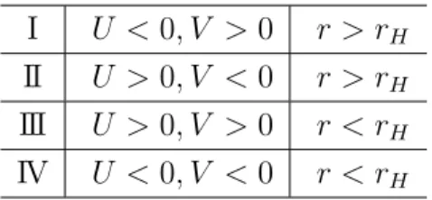
The vertical and the horizontal axises correspond to the Kruskal time T = (V + U )/2, and the Kurskal radius R = (V − U)/2. In contrast to the Schwarzschild coordinates, the Kruskal coordinates are regular beyond the horizon (r = rH), and can be extended to the maximally extended Schwarzschild space-time (−∞ < U, V < ∞). The original Schwarzschild coordinates (−∞ < t < ∞, r^H < r < ∞), on the contrary, can cover only the region I in fig.2. We define (t, r_∗) coordinates in other regions. For example, in the region II, we can define them by the relations U = e^−κ(t−r^∗⁾_{/κ, V = −e}^κ(t+r^∗⁾/κ. In the Kruskal coordinates, the space-time is separated by the future and past event horizons (U = 0 and V = 0 respectively) into four regions. There are four possible combinations of signature of U and V as shown in the table 4.1.

Finally we note that the time-like Killing vector ξ = ∂t is written as ξ = κ(V ∂V ₋

U ∂U) = κR∂T in the Kruskal coordinates and, therefore, the directions of time are opposite in the region I and II. We have drawn the directions of ξ in fig.2.

(21)

r = 0

U V

i⁺

i⁻

i0

r = rH

r =const. t =const. I

II

III

IV

Figure 2: A point in the diagram represents a two dimensional sphere with radius r at time t. r-constant and t-constant surfaces are depicted. Arrows on the r-constant surfaces indicate the flow of the time-like Killing vector. They have opposite directions in the region I and II. The singularity at r = 0 is drawn by zigzag lines in the diagram. Event horizons are located at r = rH and separate the space-time into four distinct regions. i⁺, i⁻ and i0 are the future, past and spatial infinities.

I U < 0, V > 0 r > rH

II U > 0, V < 0 r > rH

III U > 0, V > 0 r < rH

IV U < 0, V < 0 r < r_H

Table 1: Four regions of maximally extended Schwarzschild space-time

4.2 Field Theory in the Black Hole Background and the Hawk-

ing Radiation

We briefly summarize the quantum field theories in the black hole background. For a comprehensive review, see e.g. [25]. The action of a massive scalar field in the maximally extended Schwarzschild space-time is given by a sum of the fields in the right wedge (region I) and in the left wedge (region II). In each region, the action is given by

S =

∫

d⁴x^√_−g¹ 2^(g

µν_∂

µϕ∂νϕ + m²ϕ²) =^∑

l,m

∫

dtdr_∗ϕ(l,m)[∂_t²_{− ∂}_r²_∗+ Vl(r)] ϕ(l,m). (4.6)

(22)

where we have decomposed the field into partial waves ϕ(t, r, Ω) =^∑

l,m

ϕ(l,m)(t, r)

r ^Y^l,m^(Ω), ^(4.7)

and defined the effective potential for each partial wave with an angular momentum l, Vl(r) = f (r)^{( l(l + 1)}

r² ⁺

∂rf (r)

r ^{+ m}

2

)

. (4.8)

The equation of motion of the scalar field is given by

[∂_t²_{− ∂}_r²_∗ + V_l(r)] ϕR,L(l,m) ^{= 0.} ^(4.9)

Both in the asymptotically flat region (r → ∞) and in the near horizon region (r → r^H^), the potential Vl vanishes and the equation of motion is reduced to the free field equation. Thus, in the near horizon region, the classical solutions are approximately given by

u^R_k(t, r) =

{ _√1 4πωk^e

−iωkt+ikr_∗ _{(in R)}

0 (in L) ^(4.10)

u^L_k(t, r) =

{ 0 (in R)

√1 4πωk^e

iωkt+ikr∗ _{(in L).} ^(4.11)

and their complex conjugates. Here ωk = +|k| > 0. The sign difference in front of iω^k^t in R, L follows the convention of [25]. With this convention, these fields are positive frequency modes with respect to the time-like Killing vector, ∂t in R and −∂^t ^{in L,} satisfying L±∂^tû^k = −iω^kû^k. The complex conjugates (u^R,L_k )^∗ are the negative frequency modes (in the above sense) satisfying L±∂^tû^∗k ^{= +iω}^kû^∗k. They are orthonormal with respect to the following Klein-Gordon inner product,

(f, g) ≡ i

∫

Σt

d³x√hΣt(f^∗∂t_{g − ∂}tf^∗g)

= i^∑

l,m

∫

dr_∗(f_(l,m)^∗ ∂tg(l,m)_{− ∂}tf_(l,m)^∗ g(l,m)) . (4.12)

The integration is performed on a constant time slice Σt, but it can be generalized to any space-like surface Σ and the choice of the integration surface does not change the value of the inner product.

The field ϕ(l,m)can be expanded in terms of the classical solutions in the Schwarzschild coordinates in the near horizon region as follows;

ϕ_(l,m)=

∫ _dk

√4πωk

[a^R_k(l,m)u^R_k + (a_k(l,m)^R )^†(u^R_k)^∗+ a^L_k(l,m)u^L_k + (a^L_k(l,m))^†(u^L_k)^∗] . (4.13)