Noncoding Sequences ((NSs) in Eukaryotes
Nadeeka Nilmini Hettiarachchi
)octor of Philosophy
)epartment of Genetics
School of 1ife Science
SO0EN)AI (The Graduate University for
Advanced Studies)
I
Heterogeneous characteristics of
Conserved Noncoding Sequences (CNSs) in
Eukaryotes
By Nadeeka Nilmini Hettiarachchi
I
Acknowledgements
I am indebted to all those who assisted me in numerous ways, throughout the past several years, filled with hard work and tasking times. I owe everyone who were there by me and guided me with their thoughtful remarks, probing, challenging questions and suggestions including those who assisted me in numerous ways with life and living in Japan. Although one page acknowledgement would not suffice to express my sincere heartfelt gratitude to all those who sincerely meant my well- being, their names and deeds will always find room in my heart.
First I wish to extend my sincere gratitude to Prof. Naruya Saitou for his valuable advices and support during the time of my research. Thank you very much for your encouragement and patience.
Next I wish to thank my committee members, Prof Kakutani Tetsuji, Prof. Nori Kurata, Prof. Asao Fujiyama and Associate Prof. Kazuho Ikeo for their indispensable suggestions and support during the gradual progress of this study. Also I am sincerely thankful to Associate Prof. Naoki Osada of Hokkaido University for various advices during his term as one of the committee members when he was in National Institute of Genetics.
At the same time I am thankful to the members in my lab for creating a pleasant working environment. Also I wish to extend my sincere gratitude to Mr. Isaac Adeyemi Babarinde for his constant support and consideration at all times.
I am sincerely obliged to thank the Ministry of Education, Sports, Culture, Science and Technology of Japan for providing me this opportunity to pursue my graduate studies in Japan.
Finally, to my parents, my brothers and my dearest friend Morteza Mahmoudi Saber who helped me maintain a proper perspective through times of adversity, I can no more than reaffirm my sincere gratitude and devotion to them.
II
Table of Contents
Acknowledgement……….…I List of figures……….….VI
List of tables……….…VIII
List of abbreviations………...IX Abstract………..…..X
Chapter 1
Introduction………...…..…1
1.1 A general overview on Conserved Noncoding Sequences (CNSs)………...1
1.2 Conserved noncoding sequences in animal genomes………4
1.3 Progression of conserved noncoding sequence studies in plant genomes……….7
1.4 Objectives of this study……….9
1.5 Overall map of the Dissertation………...11
Chapter 2
Determination of lineage specific plant CNSs……….……12
2.1 Introduction………..12
2.2 Materials and Methods………14
2.2.1 Genomes considered in the analysis……….14
III
2.2.2 Identification of common CNSs………...14
2.2.3 Identification of lineage-specific CNSs ………..….16
2.2.4 Identification of CNSs for all pairs of species………..18
2.2.5Analysis of protein coding genes………...21
2.2.6 Characterization of the CNSs……….………..22
2.3 Results……….……....23
2.3.1 Lineage specific CNSs………..…………23
2.3.2 Lineage specific CNSs and lineage specific genes……….…..28
2.3.3 Lineage specific loss of ancestral CNSs……….……..28
2.3.4 The genomic locations of identified lineage-specific CNSs……….…32
2.3.5 Distribution of the CNSs in chromosomes……….…..35
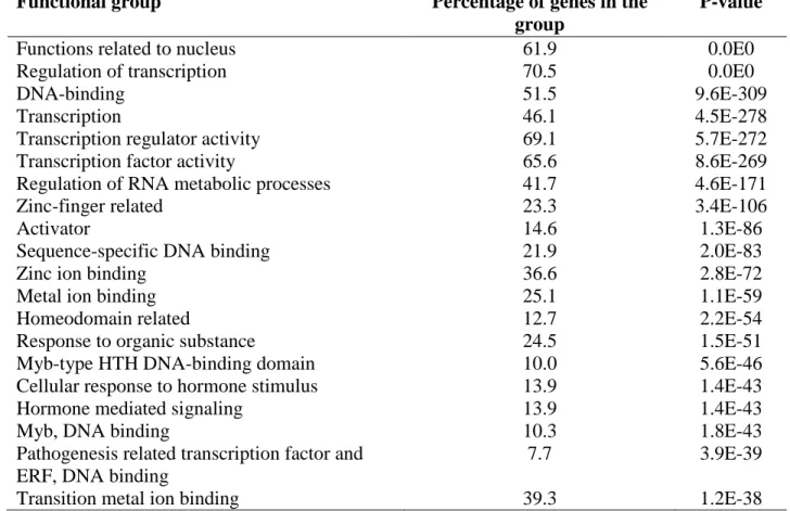
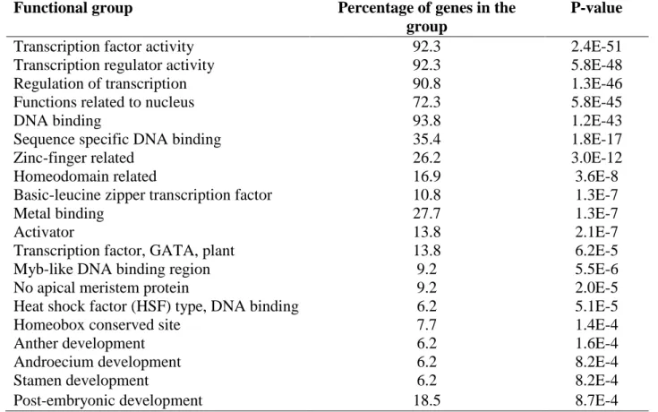
2.3.6 Predicted target genes of CNSs and their enrichment analysis………36
2.3.7 Synteny of target genes………40
2.3.8 A+T content in the flanking regions of CNSs………..40
2.3.9 Prediction of nucleosome positioning………..41
2.3.10 CNSs are not related with recombination hotspots………47
2.3.11 Methylation in eudicot specific CNSs………47
2.3.12 Phylogenetic tree construction with CNSs……….48
2.4 Discussion………..………...…..51
IV
Chapter 3
Determination of GC content heterogeneity of CNSs in Eukaryotes………...56
3.1 Introduction………..…56
3.2 Materials and Methods……….59
3.2.1 Genomes considered in the analysis……….59
3.2.2 Identification of lineage common CNSs………..59
3.2.3 Setting percentage identity cutoff for the CNSs……….………..62
3.2.4 Determining GC content of CNSs and the reference genome………..63
3.2.5 Determining ancestral GC of CNSs and background noncoding regions……….. 3.2.6 Substitution pattern determination for CNSs………63
3.2.7 GC content distribution in the flanking regions and inside of CNSs………63
3.2.8 Isochore-like regions identification………..64
3.2.9 Determination of nucleosome occupancy probability………..64
3.2. 10 Association of histone modifications with CNSs……….…….64
3.2.11 Predicted target genes of CNSs………..65
3.2.12 Transcription factor binding site (TF binding site) analysis for the CNSs in vertebrates………..65
3.2.13 Transcription factor binding site analysis for plants………..……….66
3.3 Results……….67
3.3.1 Fungi lineage common CNSs………...…………67
……….. 63
V
3.3.2 Invertebrate lineage common CNSs……….67
3.3.3 Non-mammalian vertebrate lineage common CNSs……….68
3.3.4 The pattern observed in GC content transition……….72
3.3.5 Nucleosome occupancy and GC content distribution for CNSs…………...76
3.3.6 Histone modifications related with CNSs……….…88
3.3.7 The predicted target genes for CNSs and functional classification…..……88
3.3.8 Transcription factor binding site analysis for vertebrates……….91
3.3.9 Transcription factor binding sites in plants………..…….92
3.3.10 The GC content transition in the vertebrate lineage………...93
3.4 Discussion………..….98
Chapter 4
Conclusion………....101
References………...107
Appendix………...120
VI
List of figures
Figure 2.1 - The flow charts of the lineage specific CNS determination………...19
Figure 2.2 - Example schematic diagram for identification of CNSs for all pairs of species…...21
Figure 2.3 - Phylogenetic tree with the number of lineage specific CNSs……….28
Figure 2.4 - The lineage specific loss of ancestral CNSs………...32
Figure 2.5 - CNSs found from all pairwise searches………..33
Figure 2.6 - Distribution of A+T content in the flanking regions and within CNSs (for grass specific CNSs)……….…....45
Figure 2.7 - Nucleosome occupancy probability for grass specific CNSs including flanking regions………46
Figure 2.8 - Distribution of A+T content in the flanking regions and within monocot specific CNSs, black line shows the average A+T content in rice genome………47
Figure 2.9 - Nucleosome occupancy probability for monocot specific CNSs including flanking regions………....48
Figure 2.10 - The phylogenetic trees of the CNSs……….52
Figure 3.1 - The pipeline followed to identify the lineage putative lineage common CNSs for fungi, invertebrates and non-mammalian vertebrate species used in the analysis………....64
Figure 3.2 - Relative GC content change for the CNSs. The relative change of GC content was calculated based on the noncoding GC content for the reference genome of each lineage………...76
Figure 3.3 - GC content change in order Diptera……….…...77
Figure 3.4 - Isochore distribution for the flanking regions of CNSs and random samples………....81
Figure 3.5 - GC content distribution of the CNSs across the center of CNSs and the flanking regions. 1000th nucleotide position corresponds to the center of the CNSs……….…...85
VII Figure 3.6 - Nucleosome occupancy probability for the CNSs of different lineages…………...88 Figure 3.7 - (A) Vertebrate (H. sapien) tissue specific TFs are less shared in other lineages…....98 Figure 3.8 - Plants do not show any significant difference in sharing of tissue specific and ubiquitous TF binding sites with regards to other species (H. sapien, G. gallus, and T.
rubripes)……….…...100
VIII
List of tables
Table 2.1 - Summary of lineage specific CNSs – minimum-maximum lengths, average lengths, average percentage identity and number of CNSs longer than 100 bp………...29 Table 2.2 - Genomic locations of the grass and monocot lineage specific CNSs………...35 Table 2.3 - Genomic locations of the eudicot and angiosperm lineage specific CNSs………...36 Table 2.4 - Gene enrichment analysis for the likely target genes of grass specific CNSs……….….40 Table 2.5 - Gene enrichment analysis for the likely target genes of monocot specific CNSs...41 Table 3.1- Number of lineage common CNSs, mean and mode lengths of CNSs identified for groups fungi, invertebrate and non-mammalian vertebrates………...73 Table 3.2 - Gene ontology (GO) analysis for (A) Diptera (B) Nematode and (C) teleost fish
CNSs………...93
IX
List of abbreviations
CNSs: Conserved Noncoding Sequences UCEs: ultraconserved elements
CNEs: conserved noncoding elements UTR: Untranslated region
Ds: The distance of synonymous substitution GO: Gene Ontology
TF: Transcription factor
X
Abstract
Comparative genomics approach has made it feasible to determine potential functional elements in the eukaryote genome via computational analyses. Studies on Conserved Noncoding Sequences (CNSs) have reached its climax where the computationally discovered functional elements in genomes have also been experimentally verified where they were found to function as regulatory elements governing gene expression. CNSs have been verified to function as enhancers, and as well repressors. Earlier all noncoding region of genomes was referred to as “junk DNA” but now it became clear that some noncoding regions which are evolutionarily conserved, namely CNSs, are as important as the coding regions.
I first determined lineage specific CNSs of eudicots, grasses, monocots, angiosperms, land plants and plants. Here I identified 27, 6536, 204, 19, 2 eudicot, grass, monocot, angiosperm, vascular plant specific CNSs respectively. Average percentage identity for CNSs in all groups was more than 80% and the average length varied across groups.
Since the number of CNSs varied considerably across lineages, I tried to determine if this could be due to evolutionary rate, number of species in each group or relatively short divergence time for grass lineage. Even with pairs of species from eudicots and grasses with same divergence time, eudicots had less number of CNSs than monocots. Next I showed that the number of species in each group cannot be a reason for the difference by considering same number of species from eudicots and monocots. In this case also eudicots had less number of CNSs (69) than monocots (204). With respect to the evolutionary rate I found that eudicots have a saturated Ds (2.44) compared to grasses and monocots. If evolutionary rate played a key role in number of CNSs, lineage specific genes should follow the same pattern in abundance as CNSs. Surprisingly Eudicots had more lineage specific genes (2439) than CNSs whereas monocots and grasses (113, 444) had less lineage specific genes. I also found that UTR (untranslated region) CNSs were overrepresented with respect to other regions (introns and intergenic regions). The GO (gene ontology) analysis for the likely target genes of CNSs showed that these genes are related to transcription regulation and development. Another discovery was that CNSs are flanked by sequences showing an increase of GC content and CNSs were also GC rich. Next I tested if these high GC regions are recombination hot spots, as recombination hot spots are known to be related with high GC content in the human
XI genome. None of the CNSs overlapped with recombination hot spots, while high GC CNSs have a higher propensity to form nucleosomes.
The lineage specific plant CNSs I identified were all GC rich, but mammalian CNSs have been reported to have low GC content. CNSs of diverse lineages follow different patterns in abundance, sequence composition and location. I therefore conducted a thorough analysis of CNSs in diverse groups of Eukaryotes with respect to GC content heterogeneity. I examined a total of 55 Eukaryote genomes (24 fungi, 19 invertebrates, and 12 non-mammalian vertebrates) as to find lineage specific features of CNSs. Fungi and invertebrate CNSs are predominantly GC rich, whereas non-mammalian vertebrate CNSs are GC poor, similar to mammalian CNSs. This result suggests that the CNS GC content transition occurred from the ancestral GC rich state of invertebrates to GC poor in the vertebrate lineage probably due to the enrollment of GC poor binding sites that are lineage specific. To test how the transition of GC content could have occurred, I determined the GC contents of transcription factor (TF) binding sites and their level of conservation in outgroup lineages. GC content of CNSs also showed a correlation with the location in the genome; GC poor CNSs showed a higher probability to be located in open chromatin regions and GC rich CNSs showed a tendency to locate in heterochromatin regions. The histone modification signal analysis showed that CNSs overlapped with more H3K27Ac and H3K4Me1 compared to the random expectation. These histone marks are signatures of active enhancer regions. The predicted target genes of CNSs also agreed with the previous analysis where the most overrepresented GO term was related to transcription and development. Vertebrate ubiquitous TF binding sites are significantly GC rich compared to tissue specific ones. In contrast, plants have GC rich tissue specific binding sites compared to ubiquitous ones. This heterogeneity in GC content therefore must be attributable to TF binding sites and I found that vertebrate tissue specific TFs are more lineage specific than ubiquitous ones, whereas plant tissue specific and ubiquitous binding sites showed no significant difference in conservation implying the underrepresentation of tissue specific TFs among conserved TFs is a specific feature in vertebrate lineage.
1
Chapter 1
General Introduction
1.1 A general overview on Conserved Noncoding Sequences (CNSs)
Conserved sequences in the noncoding regions of genomes have been studied and examined for more than 20 years for their functional importance (Brenner et al. 1994; Jareborg et al. 1999; Pennacchio and Rubin 2001). Long stretches of persistently conserved regions in intron, intergenic and untranslated regions in the genomes has captured the attention of many researchers for their unique properties. In some instances these conserved noncoding regions were showing higher homology across species even than for protein coding regions (Pennacchio et al. 2006; Taher et al. 2011). Also these elements have been found spanning across diverse evolutionary times. For example Woolfe et al. (2007) documented that the conserved elements they found to span over 400 million years of evolution. I would like to call such sequences as “conserved noncoding sequences” or CNSs in this dissertation.
2 In numerous studies these CNSs have been designated in varying terms such as UCEs - ultraconserved elements (Bejerano et al. 2004), CNEs - conserved noncoding elements, HCNEs - highly conserved noncoding element (Lindblad et al. 2005), HCNRs - highly conserved noncoding regions (de la Calle-Mustienes et al. 2005), Hyper-conserved elements (Guo et al. 2008) etc. These terminologies have been adapted in each investigation based on the criteria they used for the analysis of the conserved elements. For example ultraconserved elements followed a criterion of more than 200 base conservation with 100% for very closely related species such as human and mouse. Whereas Shin et al. (2005) and Pennacchio et al. (2006) adapted a relaxed threshold of 70% identity for a set of diverse organisms.
Nonetheless their functional importance stays unhindered irrespective of the terminology. Various studies on vertebrate CNSs (e.g., Bejerano et al. 2004; Lee et al. 2010; Matsunami et al. 2010; Takahashi and Saitou 2012; Matsunami and Saitou 2013; Babarinde and Saitou 2013), invertebrate CNSs (woolfe et al. 2004; Siepel et al. 2005) and plant CNSs (Kaplinsky et al. 2002; Guo et al. 2003; Inada et al. 2003; Kritsas et al. 2012; Baxter et al. 2012; Hettiarachchi et al. 2014) reported CNSs to potentially have regulatory functions related to transcription and development. It has also been found that CNSs are under purifying selection (Drake et al. 2006; Casillas et al. 2007; Takahashi and Saitou 2012; Babarinde and Saitou 2013). Some recent studies have experimentally verified the function of CNSs (Lee et al. 2010). And also there is evidence of active histone modification signals associated with the CNSs. Zheng et al. (2010) reported that Foxp3 gene is associated with CNSs enriched with H3K4Me1, H3K4Me3 histone modification signals. These histone modifications are typically known to be related with distal enhancers and active promoter regions consecutively (Heintzman et al.2007).
Primary investigations on CNSs have mainly been focused on vertebrates, but recent studies have shown CNSs are also present in invertebrates and plants. These conserved regions of which the
3 functions are yet to be fully understood still remain an enigmatic area of discovery which is yet to be fully explained.
4
1.2 Conserved noncoding sequences in animal genomes
Conserved noncoding sequences have been identified in various organisms. One initial study on Ultraconserved elements in the human genome (Bejerano et al. 2004) kindled the curiosity of researchers with regards to conservation in the noncoding portions of the genome. Though it is expected that coding regions are conserved for their functional constraint, the noncoding conservation for long stretches with a very high percentage identity was a novel idea at the time. Bejerano et al. (2004) reported on 481 segments in the human genome longer than 200bp with 100% identity conserved across rat and mouse genomes. These segments were a combination of coding and noncoding regions with a high degree of conservation. Later numerous efforts were invested into studying CNSs in animals. It was found that these conserved regions are under purifying selection (Casillas et al. 2007) and also they are found close to genes that act as developmental regulators (Sandelin et al. 2004; Woolfe et al. 2005; Vavouri et al. 2007; Elgar 2009; McEwen et al. 2009; Lee et al. 2010; Takahashi and Saitou 2012; Matsunami and Saitou 2013; Babarinde and Saitou 2013). Lee et al. (2010) studied ancient vertebrate CNSs in bony vertebrate lineages, and CNSs they found were in abundance in tissue specific enhancers and they are likely to be cis- regulatory elements that are functionally conserved through evolution. Furthermore, C. elegans has a unique set of CNSs that are not found in vertebrates and are associated with nematode regulatory genes (Vavouri et al. 2007). Clarke et al. (2012) experimentally verified the functions of two CNSs conserved between vertebrates and invertebrates which have repression function on central nervous system and hindbrain. The functions of the CNSs have also been experimentally verified in numerous instances. Lee et al. (2011) found that many of the ancient vertebrate CNSs overlapped with experimentally verified human enhancers and their functional assay of ancient vertebrate CNSs in transgenic zebrafish embryos showed that some elements were able to recapture the mouse mid brain and hind brain expression in zebrafish. More recently Sun et al. (2015) reported that some
5 CNSs related to lhx5 gene showed expression in the forebrain region of the teleost fish. Lineage specific CNSs specifically have been verified to establish lineage specific features in taxa. Since the protein coding genes are more or less persistently conserved across lineages even with long divergence times the morphological and physiological differences of organisms might have risen from regulatory elements that are specific to each lineage (Davies et al. 2014; Hettiarachchi et al. 2014). Cretekos et al. (2008) reported that bat Prx1 enhancer increases the forelimb length of tested mice. Also the loss of an enhancer region Pitx1gene causes pelvic reduction in stickleback (Chan et al. 2010). Above mentioned are some of the evidences to support lineage specific features of organisms.
For a while it was argued that these persistently conserved sequences in the noncoding regions might merely be mutational cold spots (Clark 2001). However, Drake et al. (2006) reported that the conserved noncoding sequences are not mutational cold spots but actually under selective constraint by showing that CNSs have suppressed derived allele frequencies. Takahashi and Saitou (2012) and Babarinde and Saitou (2013) also showed this pattern in mammalian CNSs.
These numerous studies have set various selection criteria for the CNSs, such as the length, e-value and percentage identity in BLAST homology searches. Some studies have used very stringent criteria for identification of CNSs such as >100bp regions of 100% identity (Bejerano et al. 2004). Some of the other criteria being used are 70% over 100bp (Duret et al. 1993; Lee et al. 2011), 95% over 50bp (Sandelin et al.2004) and 95% over 500bp (Janes et al. 2011).
Irrespective of the selection criteria, in general, animal CNSs tend to be much longer and more abundant in number. Babarinde and Saitou (2013) reported having found about 52,000 primate specific, about 12,000 eutherian specific conserved noncoding sequences by considering sequences over 100bp and 94% identity set based on protein level conservation of genes. Kim and Pritchard
6 (2007) reported on about 82,000 mammalian specific CNSs (over 90% identity without length criteria). It is important to consider various filtering thresholds when dealing with closely related species to remove false positives from the set of putative CNSs that might appear conserved due to lack of time necessary for them to accumulate mutations and diverge.
Even though there is a plethora of documented evidence for conserved noncoding sequences in animal genomes, CNSs are not restricted to animals. CNSs have also been identified and studied in invertebrates and in plant genomes to varying degrees.
7
1.3 Progression of conserved noncoding sequence studies on plant
genomes
Initially instigated studies on plant conserved noncoding sequences focused on a limited number of orthologous genes in a set of genomes. Kaplinsky et al. (2002) compared the lg1gene in two grass species, namely maize and rice, to identify putative regulatory elements associated with this gene. They also tried to identify CNSs associated with 5 more genes (Chalcone synthase, wx1, adh1, sh2, H+ ATPase) and reported that grass CNSs are smaller and less abundant than those of mammalian genomes studied at that time. Later Guo and Moose (2003) analyzed 11 orthologous maize-rice gene pairs to identify putative regulatory elements in their flanking noncoding regions. And the CNSs they identified had a minimal length of 20 bases. Inada et al. (2003) reported the first comparatively large scale analysis in to grass CNSs. This study included 52 annotated maize-rice genes considering 1000bp or more toward the promoter region of each gene and reported that the majority of the genes in the analysis at least had one CNS and most CNSs were short as less than 20 bases in length. This analysis agreed with what was reported by Kaplinsky et al. (2002). Still late into 2012 the plant CNS studies stayed limited to gene wise analyses which considered the upstream region of the genes of interest in search of regulatory elements. As genome sequencing expanded and more plant genomes became available plant CNS studies started to gain pace.
On the contrary to the previous studies that were restricted to a limited set of orthologous regions, I started my analysis on CNSs in plant genomes in 2011considering 15 species.
Kritsas et al. (2012) analyzed complete genomes of four species (Arabidopsis thaliana, Vitis vinifera, Brachypodium distachyon, and Oryza sativa), and identified ultraconserved like elements. They identified 36 highly conserved elements with at least 85% identity and are longer than 55bp between Arabidopsis thaliana and Vitis vinifera and also 4572 highly conserved elements between Oryza sativa and Brachypodium distachyon.D’Hont et al. (2012) compared Brachypodium
8 distachyon, Oryza sativa and Sorghum bicolor and identified 16,978 CNSs which were defined as pan-grass CNSs. Further with the addition to Musa acuminata they identified 116 CNSs in the commelinid monocotyledon lineage. Both these studies have concentrated on CNSs that are commonly found in the groups of species in their analyses, and also these CNSs might also be present in other lineages. Haudry et al. (2012) reported on conserved noncoding sequences responsible for crucifer regulatory network. Hettiarachchi et al. (2014) found that grasses and monocots generally had more linage specific CNSs compared to eudicots.
Similar to CNS analyses on other organisms Plant CNS studies also found that the predicted target genes of the CNSs are related to transcription regulation and DNA binding (Kritsas et al.2012; Hettiarachchi et al. 2014)The plant CNSs are also found to be enriched in transcription factor biding sites (Hettiarachchi et al. 2014; Burgess and Freeling 2014). Haudry et al. (2012) further reported that the 44% of the CNSs they identified overlapped with DNase I hypersensitive sites implying regulatory activity. Function wise plant and animal CNSs seem to be following the same pattern but the lengths and abundance of CNSs seem to vary widely between animals and plants. Even though many efforts have been invested into functionally verifying the importance of the CNSs in animals, plant CNSs are not extensively studied or analyzed with respect to function. This is one aspect of plant CNS analyses that is yet to be fully examined and expanded if we need to fully understand the regulatory architecture of plant genomes.
9
1.4 Objectives of this study
So far some of the documented CNS studies emphasize on lineage specificity brought about by regulatory elements that are unique to a particular taxa or clade. Mainly these studies have focused on vertebrate genomes (e.g., Takahashi and Saitou 2012; Matsunami and Saitou 2013; Babarinde and Saitou 2013) and elaborated on lineage specific characteristics related to vertebrates that must have driven their unique features.
There have also been studies on lineage specific expression of experimentally verified regulatory elements such as enhancer element related with Olig2 (Sun et al. 2006) that drive expression in ventral spinal cord of tested transgenic mice and further they report this element is responsible for lineage specific expression in motor neurons. Also craniofacial enhancer I37-2 is therian specific and it has contributed to the craniofacial development in the mammalian lineage (Sumiyama et al. 2012).
These evidences propose the existence of the lineage specific regulatory architecture that governs group specific features. Computational comparative genomics analyses on DNA level is the first approach to uncover such regions that are conserved throughout evolutionary history. Finding conservation in the noncoding regions of genomes through computational analyses draws the baseline in identifying such potential regulatory elements. This idea of lineage specificity with regards to conserved noncoding sequences in plants has not been tested or adapted before. This prompted me to uncover the lineage specific conserved noncoding sequences that are most likely to be putative regulatory elements of plants and also to elaborate on the CNS features compared to vertebrates.
10 In chapter 1 I address the lineage specificity of CNSs in several plant taxa namely eudicots, grasses, monocots, angiosperms, land plants and plants. The initial objectives of the first part of the study was,
To identify the CNSs that presumably originated in their respective common ancestors
Determine likely target genes and their potential functions
Determine any abundance differences in the lineage specific CNSs
Determine specific characteristics of these CNSs with regards to o Dinucleotide distribution in and around CNSs
o Relationship of CNSs and nucleosome occupancy o CNSs with regard to methylation level
Identify patterns of lineage specific loss of ancestral CNSs
Identify patterns of lineage specific CNSs and lineage specific genes
I focused on the GC content heterogeneity of CNSs across different lineages such as fungi, invertebrates, non-mammalian vertebrates and plants in Chapter 2. As identified in Hettiarachchi et al. (2014) plant CNSs are GC rich. Babarinde and Saitou (2013) showed that mammalian CNSs they identified are GC poor. This lineage difference in GC content is the main focus of this chapter. Objectives of this study involved
Determining the origin of the GC poor CNSs
Various characteristic features of CNSs belonging to different lineages
Plausible reasons for GC content heterogeneity
All the analyses were performed via custom made perl scripts which were produced by myself and genome data were retrieved from public genome repositories.
11
1.5 Overall map of the Dissertation
This dissertation all together entails four chapters with two main chapters that address different aspects of conserved noncoding sequences in organisms.
Chapter 1(this chapter) is documented to give a general overview of conserved noncoding sequences, the development of CNS studies throughout the years with regards to animal and plant CNSs.
Chapter 2 mainly deals with the analysis of the lineage specific conserved noncoding sequences in plant genomes belonging to various taxa. This chapter is fragmented into subdivisions that handle the materials and methods, results and discussion and is intended to answer the objectives listed in section 1.4. Chapter 2 has been published in Genome Biology and Evolution in 2014 September (doi: 10.1093/gbe/evu188).
Chapter 3 was documented with the expectation of answering the key question that arose with regards to CNS GC content heterogeneity of different lineages. This chapter tries to elaborate the work flow to the analysis, results based on GC contents of CNSs of different lineages, discussion and a conclusion for GC content heterogeneity of CNSs in diverse taxa.
Chapter 4 was written to summarize the discussions from chapter 2 and 3, explain plausible reasons to the observations and analyses and finally give a description on future directions with regards to this study.
12
Chapter 2
Determination of lineage specific plant
CNSs
2.1 Introduction
With the ever-increasing high throughput genomic data it has become possible to understand and decipher the genomic properties and evolutionary aspects of various organisms. The handling of genomic data on various levels has made it possible to elucidate the properties of organisms on a functional level. Comparative genomic analyses have been considered to identify conserved potential regulatory elements through varying divergence times. This has been a sound method in identifying elements that are conserved on sequence level. It has been found that these CNSs that are computationally discovered are also functionally important in shaping the morphological and physiological aspects of an organism (Sun et al. 2015; Ritter et al. 2010).Many studies have been
13 conducted in CNSs on animals and this study intended to set light on lineage specific conserved noncoding sequences in plants for the first time.
In this study I decided to focus on whole genome analysis of available plant genomes to identify lineage specific CNSs. My focus of this study is in finding all the CNSs, thus find potential regulatory elements specific to different plant lineages.
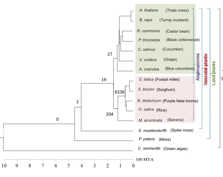
Here I searched eudicot lineage specific CNSs by analyzing genome sequences of the following seven eudicot species: Arabidopsis thaliana, Brassica rapa, Populus tricocarpa, Ricinus communis, Vitis vinifera, Cucumis sativus, and Aquilegia coerulea. To determine grass specific CNSs, genome sequences of Oryza sativa, Brachypodium distachyon, Sorghum bicolor, and Setaria italica were compared. The genome sequences of Musa acuminata were also analyzed to determine monocot specific CNSs in addition to the four grass species mentioned above. It has to be noted that in order to look for the specific CNSs in the analysis I have included the most basal species sequenced so far, assuming that if a CNS is present in the most diverged species, it is highly likely to be found in closer species inside a group. The most basal eudicot species used in the study is A. coerulea which diverged about 120 mya (Anderson et al. 2005) from the rest of the eudicot species used in this study. Musa acuminata is considered as the basal monocot species, which diverged from grasses about 115 mya (D’Hont et al. 2012). The other species used in the study are Selaginella moellendorffii which diverged from angiosperms about 400 mya (Banks et al. 2011), Physcomitrella patens which diverged 450 mya (Rensing et al. 2008) from vascular plants and Chlamydomonas reinhardtii that diverged from land plants more than 1000 mya (Heckman et al. 2001). A total of 15 species (see Figure 3 for their phylogenetic relationship) were used with the expectation of finding the group specific CNSs in this study.
14
2.2 Materials and Methods
2.2.1 Genomes considered in the analysis
Repeat masked genome sequences of Arabidopsis thaliana, Brassica rapa, Populus tricocarpa, Oryza sativa, Brachypodium distachyon, Sorghum bicolor, Selaginella moellendorffii, Chlamydomonas reinhardtii and Physcomitrella patens were downloaded from Ensembl release 12, whereas Ricinus communis, Vitis vinifera, Cucumis sativus, Aquilegia coerulea, Setaria italica were downloaded from Phytozome version 8.0. Genome sequences of Musa acuminata were downloaded from banana genome project database. Since the analysis was focused on the Conserved Noncoding Sequences (CNSs) in the nuclear DNA, the mitochondria and chloroplast genomes were removed from the analysis where they were known and annotated in the databases. Since there is also a possibility of mitochondrial and chloroplast sequences being transferred into nuclear genome, I further removed any sequences which showed homology to mitochondrial or the chloroplast genome before initiating any analyses on the respective sequences.
2.2.2 Identification of lineage common CNSs
Common to eudicots: BLAST 2.2.24+ (Altschul et al. 1997) was used for performing homology searches in this study. BLASTn search was done with A. thaliana as the query and B. rapa as the subject database. The cut off e-value for the search was 0.001. Only the alignments without any overlap with a coding region for both query and subject were used for subsequent analysis. From the remaining (nuclear DNA) BLAST hits, the best hits of overlapping alignments were selected using the e-value. If the coordinates of two sets alignments overlapped with each other
15 only the alignment with the lower e-value was retained. Thus a dataset with the best alignments for A. thaliana and B. rapa conserved noncoding sequences was produced for further analysis. The obtained best hits were searched against C. sativus, thus A. thaliana, B. rapa and C. sativus best hits were obtained the same method explained above. Similarly, the best hits of A. thaliana, B. rapa, C. sativus were searched against P. tricocarpa. This method was carried out in form of a chain (best hits of previous step used to search a new species) for the following species, R. communis, V. vinifera and A. coerulea in the sequence given, to obtain the common CNSs to eudicots. These CNSs were in turn searched in Rfam v10.1 (June 2011) and the CNSs with overlaps with noncoding RNA were removed from further analysis.
Common to grasses: BLASTn search was done with O. sativa as the query and B. distachyon as the subject database. The cut off e-value for the search was 0.001. Only the alignments without any overlap with a coding region for both query and subject were used for subsequent analysis. The remaining hits were filtered based on the e-value and only the best hits were retained to search against S. italica. Then O. sativa, B. distachyon and S. italica best hits were searched against the last monocot genome, S. bicolor. This procedure finally achieves the CNSs that are found in all the monocots used in the study and thus were considered as grass common CNSs. The common CNSs were searched in Rfam v10.1 (June 2011) and the CNSs with overlaps with noncoding RNA were removed from further analysis.
Common to all monocots: The grass-common CNSs discovered from the previous step were searched in M. acuminate to obtain CNSs that are common in all monocot species used in the study. The cut off e-value for the search was 0.001.
Common to all angiosperms, to all vascular plants, and to all plants: The eudicot common and monocot common CNSs were searched against each other with a cut off e-value of
16 0.001, using the eudicot common CNSs as the query and the monocot common CNSs as the subject, and the best hits selected based on the e-value were searched in S. moellendorffii which is a lower vascular plant in order to identify the CNSs common to vascular plants. The best hits from this step were searched in P. patens to identify any CNSs that could still be remaining as common to all land plants. Finally the best hits from this step were searched in C. reinhardtii with the expectation to find any noncoding sequences conserved in the group viridiplantae irrespective of their long divergence time.
2.2.3 Identification of lineage-specific CNSs
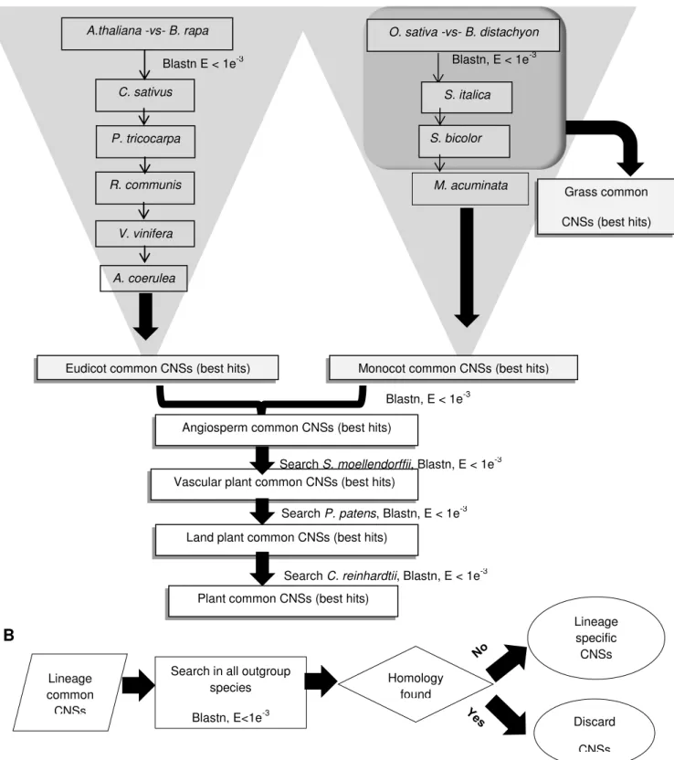
Eudicot, monocot, angiosperm, vascular plant lineage-specific CNSs: All the eudicot common CNSs found, were searched in all the outgroups used in the study (all the monocot species, S. moellendorffii, P. patens and C. reinhardtii) The CNSs that are common to eudicots and not found in any of the outgroups were designated as eudicot-specific CNSs. Similarly, in order to identify monocot specific CNSs, the monocot common CNSs were searched in the following outgroups, all the eudicots, S. moellendorffii, P. patens and C.reinhardtii used in the study. The angiosperm specific, vascular plant specific and plant specific CNSs were identified the same way by searching against their outgroups. The flowchart for the analysis is depicted in Figure 2.1.
17 A
B
Figure 2.1 - The flow charts of the lineage specific CNS determination. (A) Flow chart for lineage common CNS determination. (B) The Flow chart for lineage specific CNS determination.
A.thaliana -vs- B. rapa
Blastn E < 1e-3 C. sativus
P. tricocarpa
R. communis
V. vinifera
O. sativa -vs- B. distachyon Blastn, E < 1e-3
S. italica
S. bicolor
M. acuminata
Eudicot common CNSs (best hits) Monocot common CNSs (best hits)
Grass common CNSs (best hits)
Blastn, E < 1e-3 Angiosperm common CNSs (best hits)
Vascular plant common CNSs (best hits)
Search S. moellendorffii, Blastn, E < 1e-3
Land plant common CNSs (best hits)
Search P. patens, Blastn, E < 1e-3
Plant common CNSs (best hits)
Search C. reinhardtii, Blastn, E < 1e-3 A. coerulea
Search in all outgroup species Blastn, E<1e-3
Lineage specific CNSs Homology
found
Discard CNSs Lineage
common CNSs
18 Lineage specific loss of CNSs: One main reason for the differences in abundance of lineage- specific CNSs is partially due to retention or loss of ancestral CNSs. Consideration of ancestral CNSs give a comprehensive outline of the dynamics of the retention or loss of CNSs. To study the loss of ancestral CNSs I considered C. reinhardtii as the basal species for all land plants for this analysis. I conducted independent homology searches for all the in-group species, namely A. thaliana, B. rapa, R. communis, P.tricocarpa, C. sativus, V. vinifera, A. coerulea, S. italica, S. bicolor, B. distachyon, O. sativa japonica, M. acuminata, S. moellendorffii and P. patens with C. reinhardtii as the query genome. Hits overlapping with any genes were filtered out and then a superset of all the ancestral CNSs found in all in-group species was made by merging overlapping hits. This superset represents the aggregate of ancestral plant CNSs that are still found in C. reinhardtii. Based on this set of CNSs, the ancestral CNSs lost in each branch were found.
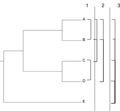
2.2.4 Identification of CNSs for all pairs of species
I conducted an analysis to determine CNSs that are present in all pairs of species and their common ancestors to provide a comprehensive view on presence of CNSs in each pair of species. In total 105 searches were performed for this analysis between different pairs of species. The cut off e-value for the search was 0.001. Only the alignments without any overlap with a coding region for both query and subject were considered. The Schematic representation of this analysis is depicted in Figure 2.
19 Figure 2.2- Example schematic diagram for identification of CNSs for all pairs of species.
This schematic example with 5 species (A, B, C, D and E) shows how the pairwise searches are performed to determine the union of CNSs for each pair of species and separate lineages. In the example the searches are performed in three levels (1, 2, and 3). The bars on the right side connecting species represent separate searches. For all the species used in the analysis a total of 105 searches were performed in a similar manner to determine the CNSs present in all pairs.
1 2 3
20
2.2.5Analysis of protein coding genes
Predicted target genes of CNSs: The gene that lies closest to a particular CNS was considered as the likely target gene. For CNSs that were found inside a gene in intron or UTR, the gene it resides was considered as the likely target gene. The likely target gene is with respect to the reference genomes used in the study. For monocot and grass specific CNSs O. sativa japonica was considered as the reference genome and for eudicot specific CNSs A. thaliana was the reference genome. These genomes have better genome annotation and quality, therefore were considered as the reference.
Identification of lineage specific genes or orphan genes: To establish a preliminary understanding of any correlation between lineage specific CNSs and lineage specific genes, I determined the numbers of lineage specific genes for eudicots, monocots and grasses. I considered protein coding gene sequences of all eudicot and monocot species used in the analysis to run blastp searches. The cut off e-value used was 0.00001 following Yang et al. (2013). The blastp searches were performed as in CNS search in a step wise manner. The lineage specific genes are defined as genes found in all the in group species but absent in all the outgroup species. It has to be noted that this analysis solely depends on the annotated protein coding sequences and that I might have missed on some unannotated genes.
Gene enrichment analysis for the likely target genes: In order to identify the functional groups for the likely target genes the gene enrichment analysis was carried out for grass and monocot specific CNSs using The Database for Annotation, Visualization and Integrated discovery (DAVID) by Huang et al. (2009).
21
2.2.6 Characterization of the CNSs
A+T content in the flanking regions and the inside of CNSs: Another analysis to characterize CNSs was done by exploring the A+T content in 1000bp flanking regions and the center (20bp) of grass and monocot specific CNSs by a moving window analysis (10bp window with 1 base step size). CNSs with flanking regions that ran into coding regions were removed from the analysis, altogether 4993 grass specific CNSs and 188 monocot specific CNSs were considered for this analysis. The statistical significance was assessed by t-test.
Nucleosome occupancy probability: Kaplan et al. (2009) built a probabilistic model of sequence preferences of nucleosome regions. This model considers the dinucleotide signals along with specific pentamer sequences that are favored or disfavored in known nucleosome sequences to produce a score for each sequence under study. I downloaded their program from http://genie.weizmann.ac.il/software/nucleo_prediction.html.
Nucleosome occupancy probabilities for grass and monocot specific CNSs were computed by considering a 4000 base region to each side starting from the center of the CNSs by using this probabilistic model. The average nucleosome occupancy probability was then computed for both sides of each nucleotide site (in total of 8000 sites) along the length of sequences. The same analysis was carried out for a random sample with same AT content as the CNSs (random sequences to have the same length as the CNSs) and also for a random sample with no specific AT preference. These random samples contained the same number of sequences as the CNSs and also same lengths with additional extending flanking regions. All the sequences were extracted from the noncoding regions of the rice genome. The average occupancy probability was calculated for all the 8000 sites for all random sequences. Statistical significance was determined by using t-test.
22 CNSs and recombination hot spots: The eudicot specific CNSs were searched against recombination hot spot data for A. thaliana published by Horton et al. (2012).
Methylation marks on eudicot specific CNSs: Further methylation marks for eudicot specific CNSs were determined by using bisulphite sequencing data for A. thaliana published by Cokus et al. (2008) and is available via http://epigenomics.mcdb.ucla.edu/BS-Seq/.Twenty seven random samples of 27 sequences in each with the same lengths as eudicot specific CNSs were extracted from the noncoding regions of A. thaliana and were searched for methylation marks. The eudicot specific CNSs and the random samples were compared with two proportion z-test at 95% confidence level.
Phylogenetic tree reconstruction with CNSs: The multiple sequence alignments were constructed for the lineage specific CNSs. The aligned multiple sequences were concatenated and the neighbor-trees (Saitou and Nei 1987) for eudicots, grasses, monocots and angiosperms were constructed with MEGA version 5 (Tamura et al. 2011).
23
2.3 Results
2.3.1 Lineage specific CNSs
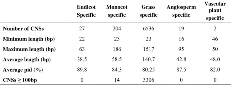
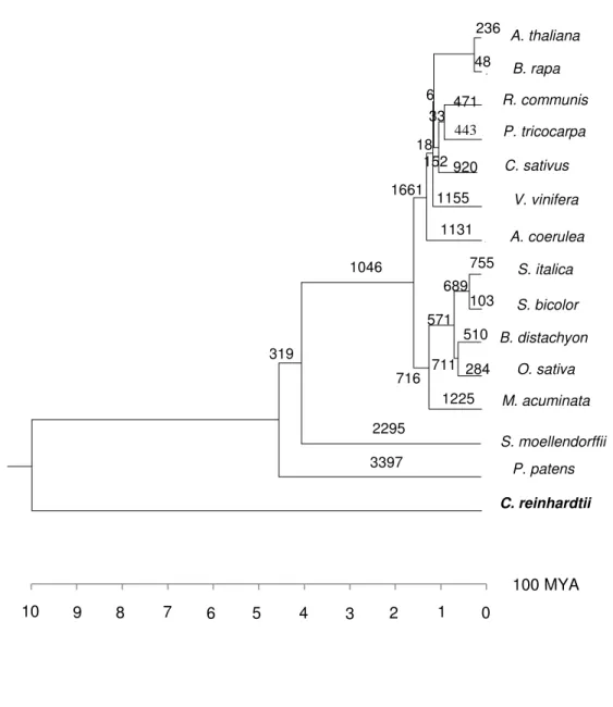
I identified 27 eudicot, 6536 grass, 204 monocot, 19 angiosperm, 2 vascular plant specific CNSs (Figure 2.3) and these lineage specific CNSs are likely to have originated in their respective common ancestors. A large number of grass-specific CNSs were observed and as a whole monocots showed more lineage specific CNSs than eudicots. The average lengths of lineage specific CNSs are in the range of 35-60bp except for grass-specific CNSs whose average CNS length was 140bp (Table 2.1). Length distributions of four lineage-specific CNSs are shown in Figure 5. Although most of lineage specific CNSs are shorter than 100bp, 3306 grass-specific CNSs and 14 monocot- specific were longer than 100bp, and the longest grass-specific CNS was 1517bp (Table 2.1). The minimum length for CNSs spans from 16 to 46bp for all lineage specific CNSs. The average percentage identity for all the lineage specific CNSs was found to be more than 80% sequence similarity.
The average percentage identity for each length groupings for CNSs provided in Appendix A1shows that the shorter CNSs have higher percentage identity leading up to >90% and have a higher conservation level while the longer CNSs tend to have lower conservation level. It should be noted that distinction between one long CNS with varying degrees of conservation and a cluster of short CNSs separated with short non conserved regions is not easy. Therefore, a change in the definition of CNSs by varying thresholds, the CNS length distribution may change.
The difference in the number of CNSs may be due to evolutionary rate differences of the lineages. In order to get an understanding if evolutionary rate could contribute to the differences, I
24 calculated the synonymous substitutions (Ds) between the reference genome and the most basal species inside the lineage. Eudicots have a very high saturated Ds value of 2.4363, while monocots and grasses have lower Ds values of 1.5118 and 0.6304, respectively. Therefore evolutionary rate could possibly be one contributing factor for the heterogeneity in number of CNSs.
Can the short divergence time be the reason for the high number of grass specific CNSs? To address this issue I selected pairs of species from eudicots and grasses with approximately the same divergence time: O. sativa and S. bicolor - divergence time of 60-70 mya (Woolfe et al. 1989), C. papaya and A. thaliana - divergence time about 70mya (Woodhouse et al. 2011). I then determined the number of CNSs for each pair. The eudicot pair had 1324 CNSs whereas the grass species pair had 16,029 CNSs. Even with the approximately similar divergence times, the pattern of CNSs remained the same as for the lineage specific CNSs. I also determined if the number of species used in the analysis for eudicots be responsible for the difference in the number of CNSs between eudicots and monocots. I randomly selected 4 eudicot species (B. rapa, R. communis, C. sativus, V. vinifera) and determined the number of lineage specific CNSs for them. The number of their lineage specific CNSs was 118, which is still much less than the number of CNSs I obtained for grasses. I further selected 5 eudicot species (B. rapa, P. tricocarpa, R. communis, C. sativus, V. vinifera) which has a total of 120 million year divergence times, and determined the number of CNSs for them, in comparison with the number of CNSs obtained for the 5 monocot species in the study. The number of lineage specific CNSs for those 5 eudicot species was 69, whereas the number of lineage specific CNSs for 5 monocot species was 204. It should be mentioned that the total divergence time of these 5 monocot species is 115 million years. Even with the same number and similar divergence times of eudicot and monocots, the number of eudicot specific CNSs remain much less than monocot specific CNSs. Therefore, the difference in number of CNSs is not due to the number of compared species.
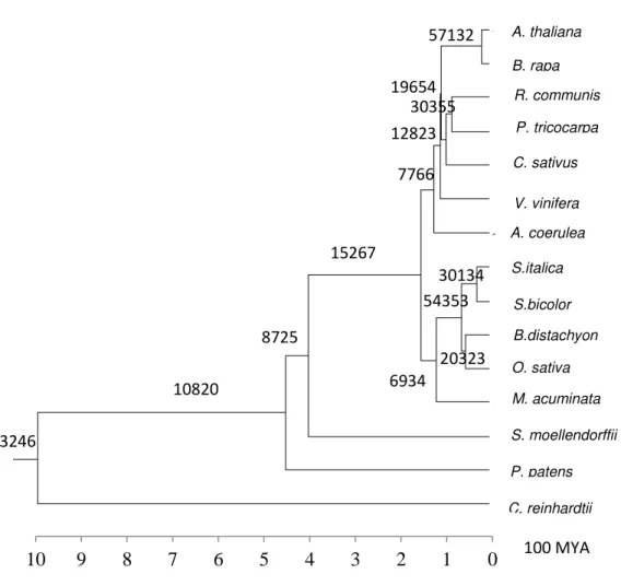
25 It is important to note that this analysis started with an initial pair of species and try to determine lineage specific CNSs for each group that are present only in all members of that lineage. But if I consider lineage common CNSs (CNSs that are commonly found in all members of a group but also might be found in out-group species; see Appendix A3), it is clear that the lineage specific CNSs are much less and represents a small fraction of elements that is likely to be functional in common ancestor. And further with this analysis to determine CNSs that are present in all pairs of species and their common ancestors (Figure 2.5) I found that the CNSs in each branch is higher (in this analyses I considered the union of CNSs) than lineage common or lineage specific CNSs. But many of these may have gone through independent losses inside a lineage, therefore would not fall under my criteria for determination of lineage specific CNSs.
26 Figure 2.3 - Phylogenetic tree with the number of lineage specific CNSs.
The numbers on each branch represents the number of lineage specific CNSs found in the study. The main plant groups considered in the study are depicted on the right. The phylogenetic tree was constructed with verified divergence times taken from Anderson et al. (2005), D’Hont et al. (2012), Banks et al. (2011), Heckman et al. (2001), Rensing et al. (2008). Eudicots and monocots are shaded in green and light pink respectively.
100 MYA 2
0
19 27
204 6536
0
(Thale cress) (Turnip mustard)
(Black cottonwood)
(Grape)
(Blue columbine) (Castor bean)
(Cucumber)
(Banana) A. thaliana
B. rapa
R. communis P. tricocarpa C. sativus
V. vinifera A. coerulea S. italica S. bicolor
B. distachyon O. sativa M. acuminata
P. patens C. reinhardtii
27
19
204 6536 2
0
0
(Green algae) S. moellendorffii
(Moss)
(Spike moss) (Rice)
(Purple false brome) (Sorghum)
(Foxtail millet)
27 Eudicot
Specific
Monocot specific
Grass specific
Angiosperm specific
Vascular plant specific
Number of CNSs 27 204 6536 19 2
Minimum length (bp) 22 23 23 16 46
Maximum length (bp) 63 186 1517 95 50
Average length (bp) 38.5 58.5 140.7 42.8 48.0
Average pid (%) 89.8 84.3 80.25 87.5 82.0
CNSs ≥ 100bp 0 14 3306 0 0
Table 2.1 - Summary of lineage specific CNSs
28
2.3.2 Lineage specific CNSs and lineage specific genes
If the evolutionary rate had been a major contributing factor for the differences in the numbers of CNSs, the lineage specific genes should also follow the same pattern as CNSs (unless the lineage specific genes are under higher selective constraint). To investigate this scenario I determined the numbers of lineage specific genes and identified 2439, 444, 113 eudicot, grass and monocot lineage specific genes consecutively. The number of eudicot lineage specific genes is much higher than grass and monocot lineage specific genes, this is quite the opposite scenario to what was observed for lineage specific CNSs. This observation gives light that apart from evolutionary rate there should be additional factors that contribute to the differences in CNSs. If I consider individual lineages, dicots evolved more lineage specific genes whereas monocots and grass common ancestors gave rise to more lineage specific CNSs.
I also found that these lineage specific genes are predominantly plant defense related.
2.3.3 Lineage specific loss of ancestral CNSs
One factor for the differences in the number of CNSs could be the loss or retention of ancestral CNSs by either rapid divergence or complete deletion (Hiller et al. 2012). Assuming an unbiased parallel loss between the reference genome (C. reinhardtii) and the other plant species, this analysis would provide an overall pattern on the rate of loss of CNSs of all plant species used.
I found that C. reinhardtii has 4355 CNSs conserved in one or more of the species used. Based on this result the number of CNSs lost in each branch was calculated. The result shows that eudicot common ancestor has lost twice as much CNSs than the monocot or grass common ancestors which indirectly answers the heterogeneity of the lineage specific CNSs (Figure 2.4, see
29 Appendix A3 for ancestral CNSs found between C. reinhardtii and other species). Of all the eudicots, V. vinifera and A. coerulea have lost the most number of CNSs independently in their respective lineages. It was observed that within grass lineage CNS loss has been lowered in O. sativa japonica and S. bicolor.
30 Figure 2.4 – The lineage specific loss of ancestral CNSs. The values on branches represent the number of CNSs lost on that specific branch. The reference genome used for this analysis is C. reinhardtii.
B. rapa R. communis P. tricocarpa
C. sativus V. vinifera A. coerulea
S. italica S. bicolor B. distachyon
O. sativa M. acuminata S. moellendorffii
P. patens C. reinhardtii
A. thaliana 236
3397 2295 319
1046
716 1661
711 571
689 755 103 510
284 1131 1155 152
48
18
6
6
920 443 471 33
0 1 2 3 4 5 6 7 8 9 10
100 MYA 1225
0 1 2 3 4 5 6 7 8 9 10
100 MYA 1 0
3 2 4 5 7 6
5 9 8
10
100 MYA
31 Figure 2.5 - Number of CNSs found from all pairwise searches. CNSs between all pairs of species were determined to have an overall comprehensive view on gain of noncoding conservation. These pairwise analyses consider the union of all CNSs. The number on each node reflects the gain of CNSs obtained via pairwise searches. These CNSs are common to each group of species and therefore are likely to be found in out-group species.
A. thaliana B. rapa
R. communis P. tricocarpa C. sativus V. vinifera A. coerulea S.italica
S.bicolor B.distachyon O. sativa M. acuminata S. moellendorffii P. patens C. reinhardtii
3246
10820
8725
15267
6934 54353
30134
20323 7766 12823
57132
19654 30355
0 1 2 3 4 5 6 7 8 9
10 100 MYA
32
2.3.4 The genomic locations of identified lineage-specific CNSs
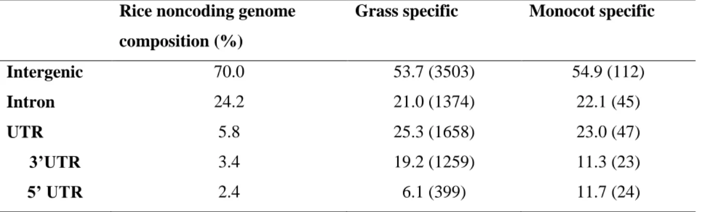
I examined the genomic locations of CNSs to see if they are in UTR, intron, or in intergenic regions. Table 2.2 shows the frequencies of these three locations of the grass and monocot specific CNSs identified with respect to the genome of O. sativa japonica as the reference. The grass and monocot specific CNSs located in the intergenic regions (53.7% and 55%, respectively) are significantly less (P-value for grass and monocots are 2.6E-161 and 0.000236, respectively) than the expectation from the genomic coverage, 70% for the reference rice genome. In contrast, the number of grass specific and monocot specific CNSs located in the UTR (25% and 22%, respectively) are significantly higher than the expectation from the genomic coverage (6%).
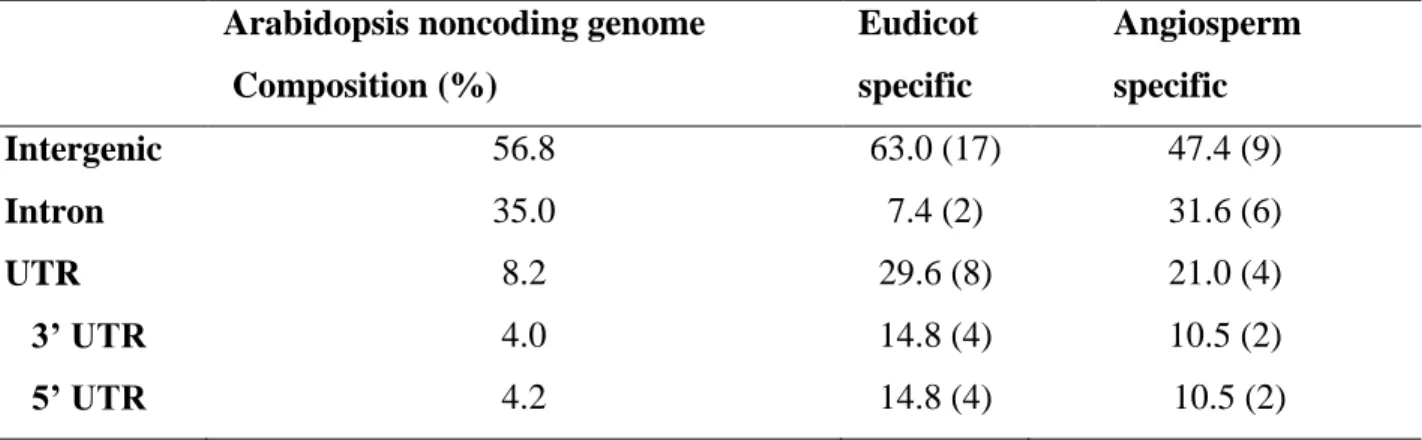
Although the eudicot and angiosperm specific CNSs are less in number, the CNSs located in the UTR regions followed a similar pattern having a significantly higher representation than the genomic coverage for the UTR regions in the reference genome (Table 2.3; A. thaliana was used as the reference genome).The result implies a stronger constraint on the CNSs located in the UTR regions.
33 Table 2.2 - Genomic locations of the grass and monocot lineage specific CNSs.
Genomic locations of grass and monocot specific CNSs with respect to the reference genome O. sativa japonica are provided as a percentage in third and fourth columns. Rough percentage estimations of the intergenic, intron and UTR regions for the reference genome are provided under rice noncoding genome composition in the second column.
Note - The exact number of CNSs in each region is given in parentheses. Rice noncoding genome
composition (%)
Grass specific Monocot specific
Intergenic 70.0 53.7 (3503) 54.9 (112)
Intron 24.2 21.0 (1374) 22.1 (45)
UTR 3’UTR 5’ UTR
5.8 3.4 2.4
25.3 (1658) 19.2 (1259) 6.1 (399)
23.0 (47) 11.3 (23) 11.7 (24)
34 Table 2.3 - Genomic locations of the eudicot and angiosperm lineage specific CNSs.
Genomic locations of eudicot and angiosperm specific CNSs with respect to the reference genome A. thaliana are provided as a percentage in third and fourth columns. Rough percentage estimations of the intergenic, intron and UTR regions for the reference genome are provided under Arabidopsis genome composition in the second column.
Note - The exact number of CNSs in each region is given in parentheses. Arabidopsis noncoding genome
Composition (%)
Eudicot specific
Angiosperm specific
Intergenic 56.8 63.0 (17) 47.4 (9)
Intron 35.0 7.4 (2) 31.6 (6)
UTR 3’ UTR 5’ UTR
8.2 4.0 4.2
29.6 (8) 14.8 (4) 14.8 (4)
21.0 (4) 10.5 (2) 10.5 (2)
35
2.3.5 Distribution of the CNSs in chromosomes
I next examined chromosomal distributions of lineage-specific CNSs. Grass and monocot specific CNSs were found distributed among all the 12 chromosomes with respect to O. sativa japonica – the reference genome (see Appendix A2 A and B for grass-specific and monocot-specific CNSs, respectively). However, the numbers of CNSs on each chromosome varied and further, intra- chromosomal distributions of the CNSs were observed to be uneven as well. One example is chromosome 10 with CNSs concentrated in several areas in reference genome for grass specific CNSs (encircled in black – 3 clear clusters). This indicates that rather than being distributed randomly, CNSs tend to exist in clusters. A similar pattern was observed for monocot specific CNSs. Some example likely target genes related to CNSs in cluster 3 are, FAD dependent oxidoreductase domain containing protein, aldo/keto reductase family protein, transcription factor BTF3, double- stranded RNA binding motif containing protein, cytokinin dehydrogenase precursor etc. Functions of some of these genes are documented to be important in regulation of genes. Even though it has been reported that much of plant BTF3 functions still remain obscure, previous researches suggest that BTF3 is associated with HR (hypersensitive-mediated) mediated cell death and involved in biotic stress regulation in the nucleus (Huh et al. 2012), and also double stranded RNA binding protein plays a vital role in viral defense and development by regulation of cellular signaling events and gene expression (Waterhouse et al. 2001).