Contributions to the theory of
weak convergences in Hilbert spaces
and its applications
SOKENDAI (The Graduate University for Advanced Studies)
Koji Tsukuda
Contents
1 Introduction and preliminaries 4
1.1 Historical backgrounds and goals of this thesis . . . 4 1.2 The organization of the thesis . . . 6 1.3 Preliminaries . . . 6 2 The weak convergence theory in separable Hilbert spaces 9 2.1 Known results . . . 9 2.2 A new criterion . . . 13
I Applications to change point tests 15
3 Introduction and the key idea 16
3.1 Historical backgrounds and rough explanations . . . 16 3.2 A change point test for an independent random variables - the
key idea - . . . 19 3.3 Bridging a gap between the independent case and stochastic
processes . . . 36
4 On convergences of some random fields 38
4.1 Limit theorems for stochastic integrals taking values in L2 spaces 38 4.2 Limit theorems for discrete time martingales taking values in
L2 spaces . . . 48
5 Continuous time stochastic processes 58
5.1 The limit distribution of Z-process . . . 58 5.2 A change detection procedure for an ergodic diffusion process . 67
6 Discrete time stochastic processes 78
6.1 The limit distribution of Z-process . . . 78
6.2 A change detection procedure for for an ergodic time series . . 89
7 Other topics 96 7.1 Z-process method and likelihood ratio process method for in- dependent data . . . 96
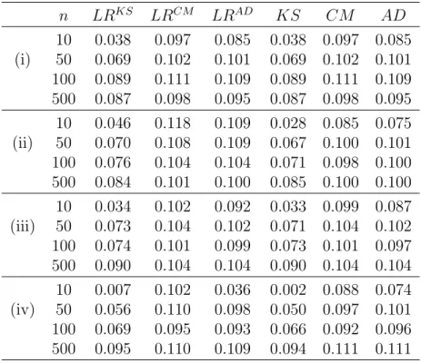
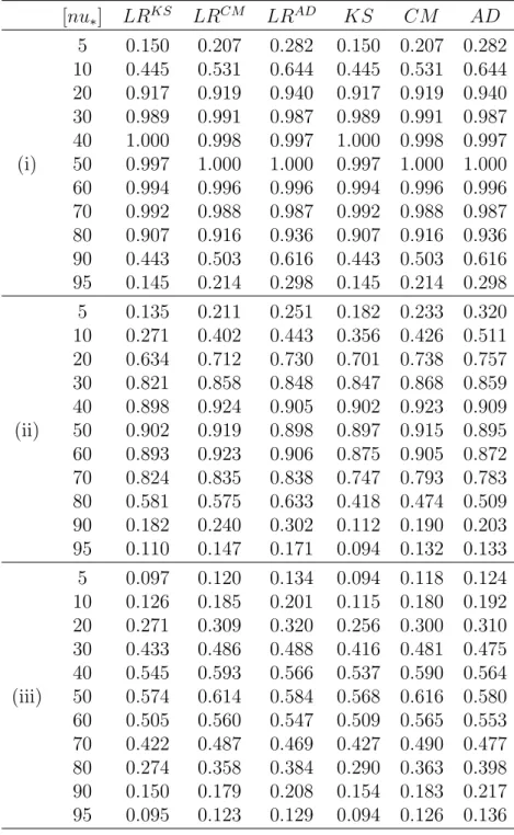
7.2 Monte Carlo simulations . . . 100
7.3 A test for a raw moment change . . . 101
II Applications to functional limit theorems for ran-
dom combinatorial structures 107
8 Introduction 108 9 The Ewens sampling formula 110 9.1 The result . . . 1109.2 A Poisson process approximation . . . 113
9.3 A functional CLT for a Poisson process . . . 119
9.4 Proof of the Theorem 9.1.1. . . 123
10 Random mappings 124 10.1 The result . . . 124
10.2 A Poisson process approximation . . . 125
Bibliography 129
Acknowledgements 135
Chapter 1
Introduction and preliminaries
1.1 Historical backgrounds and goals of this
thesis
The weak convergence theory for random elements taking values in metric spaces such as functional spaces endowed with some metrics, has been de- veloped over decades because it is of interest in itself as well as usefulness in statistical applications including goodness of fits tests and change point detection tests. Especially, a well-known goodness of fit test “Kolmogorov- Smirnov test” was validated by the so-called functional central limit theorem proven by M. D. Donsker following the heuristic approach stated by J. L. Doob, although the null distribution was originally derived by a direct cal- culation of characteristic functions much earlier. On the other hand, weak convergence theories in metric spaces were conclusively established by the landmark paper by Prohorov (1956). In that paper, a separable Hilbert space was one of concrete examples of metric spaces. After this work, the weak convergence theory in Banach spaces including a Skorokhod space D, which is the space of c`adl`ag functions endowed with the Skorokhod metric, and the space ℓ∞, which is the space of bounded functions endowed with the supremum norm, has been developed much further and applied to many problems. See the books by Billingsley (1999) and by van der Vaart and Wellner (1996). On the other hand, the weak convergence theory in sepa- rable Hilbert spaces, especially L2 spaces, has not been so developed and applied as compared to D and ℓ∞ spaces. However, an elegant treatment of the Anderson-Darling statistic written in Example 1.8.6 of the book by
van der Vaart and Wellner (1996) is of intense interest enough that it lets us foresee its extensive applicability. A possible direction is to consider de- pendent random variables. In the most previous works such as Khmaladze (1979) which considered empirical processes and Mason (1984) which consid- ered quantile processes, independent random variables were argued. Though Oliveira and Suquet (1995, 1996, 1998) and Morel and Suquet (2002) treated empirical processes for some dependent cases, associated case and mixing case, they did not consider random fields which have the Anderson-Darling type weight function. Another possible direction is to expand the field of applications. Khmaladze (1979) and LaRiccia and Mason (1986) applied the weak convergence results of empirical processes and quantile processes to goodness of fit tests. Suquet and Viano (1998) applied the results of Oliveira and Suquet (1995) to change point tests. Some other statistical applications are in Oliveira and Suquet (1996). See Oliveira (2012) for some results about functional limit theorems of associated sequences in Lp spaces, including L2 spaces, and the Skorokhod spaces.
Broadly speaking, this thesis has two goals. The one is to develop the limit theorem of random fields which have the weight function equivalent of the Anderson-Darling statistic used for testing change point hypotheses. We consider the model not only the independent random variables but stochastic processes. Especially, random fields of stochastic integrals taking values in L2 spaces are considered. This part is based on Tsukuda (2015) and Tsukuda and Nishiyama (2014, 2015).
The other goal is to derive the new functional central limit theorems in L2 spaces for the number of partitions by the Ewens partition and random mappings, which are important examples of random combinatorial struc- tures, with a weight function. Because of this weight function, ℓ∞ space may be not suitable as a framework to discuss the asymptotic behavior of random fields considered in this thesis. Because only one functional space discussed before is the Skorokhod space in this field, this thesis gives novel results. This part is based on Tsukuda (2014).
Although these two goals are concerned with different problems, there is a common treatment by the limit theorem in L2 spaces at the base of the problems. Let us call it “L2 space approach”. We expect that more new limit theorems in an L2 space can be acquired by this approach and it makes this approach valiant.
1.2 The organization of the thesis
The rest of this thesis is consisted as follows. In chapter 2, the weak con- vergence theory in Hilbert spaces is summarized and a new theorem with simple tightness criterion, which may be convenient especially for martingale random fields, is presented.
Part I is concerned with change point tests for some stochastic processes. Historical backgrounds and the key idea of our approach are explained in chapter 3. Chapter 4 contains some results on convergences of random ele- ments taking values in L2 spaces. Change point tests for continuous stochas- tic processes and discrete ones are argued in chapter 5 and 6, respectively. Chapter 7 includes comparisons of likelihood ratio methods and Z process methods and other problems for some independent cases.
Part II is devoted to L2 functional limit theorems for two famous random logarithmic combinatorial structures: the Ewens sampling formula and ran- dom mappings. This part consists of three chapters. The goal of this part is formulated and historical backgrounds are explained in chapter 8. In chapter 9, a new functional CLT for the Ewens sampling formula is presented. The proof contains verifying a Poisson process approximation in L2([0, 1], du) and establishing a functional CLT for a homogeneous Poisson process in an L2 space. In chapter 10, a new functional CLT for random mappings, which is the other problem of this part, is presented. The argument for a Poisson process approximation which is different from chapter 8 is contained.
1.3 Preliminaries
Let us make some conventions. In this thesis, convergences as T → ∞ and n → ∞ are considered. The notations →p and →d denote convergence in probability and convergence in distribution, respectively. The notation l.i.m. means the limit in the second mean, where this “mean” is meant the expectation. “The sum” ∑0k=1ak is equal to 0 for any {a·}. The notation 1{·} denotes the indicator function. The binary relations a ∧ b and a ∨ b for a, b ∈ R mean min(a, b) and max(a, b), respectively. Let us denote the transpose of vector or matrix by superscript ⊤. The i-th element of vector x is denoted by (x)(i) and the finite dimensional Euclidean norm of vector x is denoted by ∥x∥ = √x⊤x. The (i, j) element of matrix A is denoted by
(A)(i,j) and the operator norm of matrix A is denoted by ∥A∥OP, that is,
∥A∥OP = sup
x∈Rd,∥x∥=1∥Ax∥ =
sup
x∈Rd,∥x∥>0
∥Ax∥
∥x∥ . Moreover, the Frobenius norm of matrix A which is defined by
∥A∥ =√tr(A⊤A) =
√
∑
i
∑
j
|(A)(i,j)|2
is denoted by ∥A∥. Note that it holds that
∥A∥OP = maxσ σ(A)
≤
√
∑
σ
(σ(A))2 = ∥A∥
≤ ∑
i
∑
j
|(A)(i,j)|,
where σ(A) denotes the singular value of the matrix A. The expectation and the variance, or the covariance matrix, of X which has density func- tion f (x, θ) is denoted by Eθ[X], V arθ[X], respectively. In particular, for a random vector X, Eθ[X] denotes the expectation of each element of X and V arθ[X] denotes the covariance matrix of X. For a random matrix X, Eθ[X] also denotes the expectation of each element of X. The covariance of random variables X1 and X2 is denoted by Covθ(X1, X2). For these three notations, when there is no risk of confusion, we omit subscript θ.
Let us introduce a functional space L2(S, Rd, ds), or abbreviation form L2(S, ds), L2(ds) or L2(S), where S is a bounded subset of the Euclid space. Consider the inner product
⟨z1, z2⟩L2(S) =
∫
S
z1(s)⊤z2(s)ds,
where z1 and z2 are d dimensional vector-valued functions on S and ds is the Lebesgue measure. The functional space L2(S, Rd, ds) is equivalence classes of square integrable real vector functions on a bounded set S, that is, the set of all measurable functions z : S → Rd which satisfy ∥z∥2L2(S) =
⟨z, z⟩L2(S) < ∞. This space is a separable Hilbert space with respect to L2
distance d2(z1, z2) = ∥z1− z2∥L2(S). Note that ∥ · ∥L2(S) is different from ∥ · ∥, which is the Euclidean norm. In many cases, the inner product ⟨·, ·⟩L2([0,1],du) and the norm ∥ · ∥L2([0,1],du) are denoted by ⟨·, ·⟩L2 and ∥ · ∥L2 for simplicity. Let us denote a complete orthonormal system for L2([0, 1], Rd, du) space by e1, e2, . . . . Note that, for example, it can be constructed as follows: If {e′j; j ∈ J} is a complete orthonormal system for L2([0, 1], R, du),
{(e′j, 0, . . . , 0)⊤, (0, e′j, 0, . . . , 0)⊤, . . . , (0, . . . , 0, e′j)⊤; j ∈ J}
becomes a complete orthonormal system for L2([0, 1], Rd, du). The predictable quadratic variation process of martingales t ⇝ Mt is denoted by t ⇝ ⟨M⟩t
and note that it is different from the inner product ⟨·, ·⟩L2(S).
In the proofs, we sometimes omit integral region for simplicity if there is no risk of confusion.
Chapter 2
The weak convergence theory
in separable Hilbert spaces
2.1 Known results
In, this section, let us introduce the result written in van der Vaart and Wellner (1996) with the assumption of the measurability. The conditions for the weak convergence of random elements taking values in separable Hilbert space was given by Prohorov (1956). Let H be a real separable Hilbert space with inner product ⟨·, ·⟩H and a complete orthonormal system {ei}. A H- valued random sequence Xn is said to be asymptotically finite dimensional if for any δ, ε > 0, there exists a finite subset {ei : i ∈ I} of the complete orthonormal system such that
lim sup
n→∞
P (
∑
j̸∈I
⟨Xn, ej⟩2H > δ )
< ε.
This tightness criterion is established by Prohorov (1956) and the phrase
“asymptotically finite dimensional” is apparently firstly used in van der Vaart and Wellner (1996).
The weak convergence in separable Hilbert spaces is characterized by the following theorem which clearly generalizes the Cram´er-Wold theorem which characterizes weak convergences in finite dimensional Euclid spaces, see, for example, Billingsley (2012).
Theorem 2.1.1. A sequence of random variables Xn : Ωn → H converges in distribution to a tight random variable X if and only if it is asymptoti- cally finite dimensional and the sequence ⟨Xn, h⟩H converges in distribution to ⟨X, h⟩H for every h ∈ H.
See section 1.8 of van der Vaart and Wellner (1996) for more details and the proof. It should be noted that the measurability of {X·} is not assumed in their book. In this case, we have to argue the asymptotic measurability instead. By this theorem, we can prove the following CLT in a Hilbert space. Example: the central limit theorem in a Hilbert space Consider the sequence {X·} of i.i.d. random elements which take their values in a separable Hilbert space H. Assume that E[⟨X1, h⟩H] = 0 for any h ∈ H and E[∥X1∥2H] < ∞. It holds that n−1/2∑ Xk converges to a Gaussian field G which satisfies ⟨G, h⟩ ∼ N(0, E[⟨X1, h⟩2H]) for any h ∈ H.
Actually, it follows from the CLT that
⟨ 1
√n
n
∑
k=1
Xk, h
⟩
H
= √1 n
n
∑
k=1
⟨Xk, h⟩H →dN (0, E[⟨G, h⟩2H])
for any h. Moreover, letting {ej : j ∈ J} be a complete orthonormal system for H, it holds that
E
∑
j>J0
⟨ 1
√n
n
∑
k=1
Xk, ej
⟩2 H
= 1
n
∑
j>J0
E
( n
∑
k=1
⟨Xk, ej⟩H )2
= 1 n
∑
j>J0
E [ n
∑
k=1
⟨Xk, ej⟩2H ]
= ∑
j>J0
E[⟨X1, ej⟩2
H
]
= E [
∑
j>J0
⟨X1, ej⟩2H ]
converges to 0 as J0 → ∞. That is because, by the Bessel inequality, the in- tegrand (of the expectation) is bounded above by ∥X1∥2 which is integrable.
By this CLT and the continuous mapping theorem, we can derive the asymptotic distribution of the Anderson-Darling test statistic.
Example: the Anderson-Darling test statistic for the goodness of fit test Consider the sequence {X·} of real valued i.i.d. random variables with continuous distribution function F .
Let F0 be a given continuous cumulative distribution function. We wish to test:
H0: F = F0 H1: F ̸= F0
Consider the measure dF on (R, B(R)) Let us define the random field t ⇝ Zk(t) = 1{Xk ≤ t} − F (t)
√F (t)(1 − F (t))
which takes its value on L2(R, dF ). It holds that E[⟨Z1, h⟩L2(R)] = 0 and that E[∥Z1∥2L2(R)
] = 1 by the Fubini theorem. Due to the central limit theorem in a separable Hilbert space,
√1n
n
∑
k=1
Zk(·) =
√n(Fn(·) − F (·))
√F (·)((1 − F (·)) →
dG(·)
in L2(R, dF ), where the empirical distribution function of X1, . . . , Xn is de- noted by Fn and t ⇝ G(t) is a Gaussian field. It follows from the Fubini
theorem that
E[⟨Z1, h⟩2
L2(R)]
=
∫
R
∫
R
E[Z1(s)Z1(t)]h(s)h(t)dF (s)dF (t)
=
∫
R
∫
R
F (s ∧ t) − F (s)F (t)
√F (s)((1 − F (s))F (t)((1 − F (t))h(s)h(t)dF (s)dF (t)
=
∫
R
∫
R
F (s) ∧ F (t) − F (s)F (t)
√F (s)((1 − F (s))F (t)((1 − F (t))h(s)h(t)dF (s)dF (t)
=
∫
R
∫
R
E[B◦(F (s))B◦(F (t))]
√F (s)((1 − F (s))F (t)((1 − F (t))h(s)h(t)dF (s)dF (t)
= E
⟨ B◦(F (·))
√F (·)(1 − F (·)), h
⟩2 L2(R)
,
where u ⇝ B◦(u) denotes the (1 dimensional) standard Brownian bridge which is defined by B◦(u) := B(u)−uB(1) for any u, where u ⇝ B(u) denotes the standard Brownian motion. The first and the second moments of the standard Brownian bridge are given by E[B◦(u)] = 0 and E[B◦(u)B◦(v)] = u ∧ v − uv for any u, v. Therefore, in this case,
G(·) = B
◦(F (·))
√F (·)(1 − F (·)).
By the convergence above and the continuous mapping theorem, it holds that
∫
R
n(Fn(t) − F (t))2
F (t)(1 − F (t)) dF (t) →
d
∫
R
( B◦(F (t))
√F (t)(1 − F (t)) )2
dF (t)
=
∫ 1 0
( B◦(u)
√u(1 − u) )2
du.
Now, let us discuss the goodness of fit test. We can use
∫
R
n(Fn(t) − F0(t))2
F0(t)(1 − F0(t)) dF0(t)
as the test statistic. This statistic is called the Anderson-Darling (AD) statis- tic. We can construct the approximate rejection region by the asymptotic distributions under H0 derived above.
2.2 A new criterion
Sufficient conditions are given in the following proposition in order to check that a given sequence of random elements taking values in H is asymptotically finite dimensional.
Proposition 2.2.1. A sequence of random variables Xn: Ω → H is asymp- totically finite dimensional if there exists the random variable X such that
E[∥Xn∥2H] → E[∥X∥2H] < ∞ (2.2.1) and
E[⟨Xn, ej⟩2H] → E[⟨X, ej⟩2H], ∀j ∈ J, (2.2.2) as n → ∞, where {ej : j ∈ J} is a complete orthonormal system of H. Proof of the Proposition 2.2.1. It is enough to show that ∀ϵ > 0, there exists a finite subset {ei : i ∈ I} of the complete orthonormal system such that
lim sup
n→∞
E [
∑
j̸∈I
⟨Xn, ej⟩2H ]
< ϵ
by the Markov inequality. The Parseval identity yields that
∥X∥2H =∑
j∈I
⟨X, ej⟩2H+∑
j̸∈I
⟨X, ej⟩2H,
so, it holds that for any ϵ > 0 there exists a finite subset I ⊂ J such that
∑
j∈I
E[⟨X, ej⟩2H] > E [∥X∥2H] − ϵ.
Thence, we have from the assumptions that
E [
∑
j̸∈I
⟨Xn, ej⟩2H ]
= E[∥Xn∥2H] − E
[
∑
j∈I
⟨Xn, ej⟩2H ]
→ E[∥X∥2H] − E [
∑
j∈I
⟨X, ej⟩2H ]
< ϵ
for enough large finite set I. This completes the proof.
Corollary 2.2.1. If {Xn} satisfies (2.2.1), (2.2.2) and the sequence ⟨Xn, h⟩H converges in distribution to ⟨X, h⟩H for every h ∈ H, then Xn→d X in H.
It will appear easier to check this set of sufficient conditions especially for some martingales and we shall use this corollary frequently in the thesis.
Part I
Applications to change point
tests
Chapter 3
Introduction and the key idea
3.1 Historical backgrounds and rough expla-
nations
As it is written in Chapter 1, the weak convergences of random elements tak- ing values in Hilbert spaces was firstly established by Prohorov (1956). After Prohorov’s paper, the weak convergence theory in Hilbert space progresses owing to some works; for example, see Parthasarathy (1967), Jakubowski (1980), Dedecker and Merlev`ede (2003), Merlev`ede (2003) and their refer- ences. On the other hand, the applications to statistical problems seem to be much less numerous than ones of other functional spaces like ℓ∞ space, which is a space of bounded functions equipped with the supremum norm.
A successful applications of the weak convergence theory in L2 space is to derive the asymptotic distribution of Anderson-Darling (AD) test statis- tic for goodness of fit test. While the asymptotic distribution of the test statistic was derived by a direct calculation of characteristic functions in the original paper by Anderson and Darling (1952), the book for modern theo- ries of empirical processes by van der Vaart and Wellner (1996) contains an elegant proof based on the L2 limit theory. See Section 1.8 of their book, and see also Khmaladze (1979) and LaRiccia and Mason (1986). Moreover, there is an application to change point problems for independent observations with the Anderson-Darling type weight function which needs more delicate arguments: see Tsukuda and Nishiyama (2014). The important point here is that we have to treat the weight function of the form (u(1 − u))−1/2 for u ∈ (0, 1) and it preclude the use of the weak convergence theory in ℓ∞
space. In order to treat this weight function, most of the previous works of change point problems adopted the theory of Hungarian construction; we refer to Cs¨org˝o et al. (1986), Cs¨org˝o et al. (1993) and Cs¨org˝o and Horv´ath (1997) for the details. Indeed the approach by this celebrated theory gives us powerful tools in many situations, but it is not clear that we can apply it to the problems in this part, which are stated below , and we think it is natural to consider L2 space as frameworks of weak convergences in or- der to treat this weight function. There are numerous studies which treat change point problems; see Cs¨org˝o and Horv´ath (1997), Brodsky and Dark- hovsky (2000) and Chen and Gupta (2012) for reviews, and see Horv´ath and Rice (2014) for current progresses. Especially, there are several papers which treat change detections in stochastic process models; for example, diffusion processes with continuous observations: Lee et al. (2006), Mihalache (2012), Negri and Nishiyama (2012) and Dehling et al. (2014), diffusion processes with discrete observations: DeGregorio and Iacus (2008) and Song and Lee (2009), counting processes: Matthews et al. (1985) and Liang et al. (1990), AR(p) processes: Gombay (2008). Negri and Nishiyama (2014) adopts gen- eral framework called Z-process methods. However, none of them seem to have the same view as us. It is noted that although Suquet and Viano (1998) applied L2 limit theorems to change point problems for some depen- dent cases, mixing and associated cases, they proved weak convergences of some statistics which do not have a weight function (u(1 − u))−1/2.
Let us make a rough explanation of our results. Consider a parametric model {Pθ} indexed by parameter θ. Let t ⇝ Xt, t ∈ [0, ∞) be a semi- martingale whose compensator is ∫ as(θ)ds and {ξk}k=1,2,... be a martingale difference sequence under a probability measure Pθ for every θ. We shall pro- pose a general approach based on the theory of weak convergence of random elements taking values in L2spaces: for continuous time stochastic processes, consider
(u, θ) ⇝ ZT(u, θ) = √1 T
∫ T 0
wTs(u)Hs(θ)(dXs− as(θ)ds), (3.1.1) where H is a predictable process and
wsT : (0, 1) ∋ u 7→ wsT(u) = 1{s ≤ T u} − u
√u(1 − u) , s ∈ [0, T ];
and for discrete time stochastic processes, consider (u, θ) ⇝ Zn(u, θ) = √1
n
n
∑
k=1
wnk(u)Hk−1(θ)ξk(θ), (3.1.2)
where Hk−1 is a measurable-Fk−1 random element and
wkn: (0, 1) ∋ u 7→{0, u ∈(0,
1 n) , 1{k≤nu}−[nu]/n
√[nu]/n(1−[nu]/n), u ∈
[1
n, 1) , k = 1, . . . , n.
Let us call (3.1.1) and (3.1.2) pinned Z-process, because if we assign the solution, or approximate solution, of estimating equations
1 T
∫ T 0
Hs(θ)(dXs− as(θ)ds) = 0 and
1 n
n
∑
k=1
Hk−1(θ)ξk(θ) = 0
for θ, (3.1.1) and (3.1.2) equal to the partial sums of estimating equations if we attach the suitable weight functions and rate constants. Pinned Z- processes converge to centered Gaussian fields as T , or n, tends to infinity. This idea basically comes from the the work of Horv´ath and Parzen (1994). They studied the asymptotic behavior of a Fisher score change process, it is the partial sum of the likelihood equation, for general independent observa- tion cases under the null hypothesis. See also Negri and Nishiyama (2012), they refined the idea and applied it to a change detection of drift parameters in an ergodic diffusion process model. The proof for the limit theorem of Ne- gri and Nishiyama (2012), especially the proof for the asymptotic tightness, is based on the tightness criterion for martingales taking values in ℓ∞ spaces developed by Nishiyama (1999). As for the tightness criterion for martin- gales taking values in ℓ∞ spaces, see also Nishiyama (2000) and references therein. Moreover, this approach is generalized to wide class of stochastic processes by Negri and Nishiyama (2014). However, as it is stated above, we cannot apply this kinds of weak convergence theorem to the current problems because the random fields ZT and Zn are not bounded in (0, 1) with respect to u. Hence, we regard random fields (3.1.1) and (3.1.2) as the elements in some space L2([0, 1], du) and prove the limit theorems in this space.
3.2 A change point test for an independent
random variables - the key idea -
Let us describe the problem for independent observations. Let (X , A, µ) be a measure space. Let Xk, k = 1, . . . , n be independent random variables taking values in X , whose probability density functions with respect to the measure µ are f (x; θ(1)), . . . , f (x; θ(n)), where θ ∈ Θ ⊂ Rdand Θ is a bounded open convex set. For this model, what we wish to test is that
H0: ∃θ0 ∈ Θ such that θ(k) = θ0, ∀k = 1, . . . , n
H1: ∃θ0, θ1 ∈ Θ, ∃u∗ ∈ (0, 1) such that θ(k) = θ0, ∀k = 1, . . . , [nu∗] and that θ(k)= θ1 ̸= θ0, ∀k = [nu∗] + 1, . . . , n
The likelihood is given by
n
∏
k=1
f (Xk, θ(k)),
and the log likelihood is
n
∑
k=1
log f (Xk, θ(k)) =
n
∑
k=1
lθ(k)(Xk),
where lθ(x) = log f (x, θ). Consider the likelihood equation 1
n
n
∑
k=1
˙lθ(Xk) = 0.
The notation ˆθndenotes the solution, or an approximate solution in the sense that
1 n
n
∑
k=1
˙lθˆn(Xk) = oP(n−1/2), of the above equation.
Suppose the following conditions. Let us assume that lθ is second order differentiable with respect to θ. For any θ0 ∈ Θ, there exists a nonnegative measurable function K which satisfy
∫
X
K(x)f (x, θ0)µ(dx) < ∞, and
|∂ilθ1(x) − ∂ilθ2(x)| ≤ K(x) ∥θ1− θ2∥ , ∀θ1, θ2 ∈ N (3.2.1)
|∂ijlθ1(x) − ∂ijlθ2(x)| ≤ K(x) ∥θ1− θ2∥ , ∀θ1, θ2 ∈ N (3.2.2) for all i, j = 1, . . . , d, where N is neighborhood of θ0. The matrix
Iθ = lim
n→∞
1 n
n
∑
k=1
Eθ
(k)[ ˙lθ(Xk) ˙lθ(Xk)
⊤],
is assumed to be a positive definite matrix for all θ. Assume that for all i, j = 1, . . . , d, for all k = 1, . . . , n and all θ ∈ Θ,
Eθ
(k)[(∂i∂jlθ(Xk))
2] < ∞, Eθ
(k)[(K(Xk))2] < ∞, and there exist a δ > 0 such that for all i = 1, . . . , d,
Eθ
(k)
[
|∂ilθ(Xk)|2+δ]< ∞. (3.2.3) Let us assume
θ:∥θ−θinf0∥>ε
∫
X
˙lθ(x)f (x, θ0)µ(dx)
> 0, ∀θ0 ∈ Θ, ∀ε > 0. (3.2.4)
As for the estimator ˆθn, it holds that the following properties: Under H0, it holds that √n(ˆθn− θ0) →d N (0, Iθ−10 ). Under H1, it holds that ˆθn →p θ∗, where θ∗ is a point in Θ such that
θ∗ ̸= θ0, θ∗ ̸= θ1, u∗Eθ0[ ˙lθ∗(X1)] + (1 − u∗)Eθ1[ ˙lθ∗(X1)] = 0.
Here, let us explain Z-process methods. Solutions to estimating equations Ψn(θ) = 1
n
n
∑
k=1
ψ(Xk, θ) = 0
are sometimes called Z-estimators (see Chapter 3.3 of van der Vaart and Wellner (1996) and Chapter 5 of van der Vaart (1998)), where ψ(x, θ) is a finite dimensional vector. See ψ(Xk, θ) as ˙lθ(Xk) in this section. We shall consider change point tests based on estimating equations. For the purpose of it, let us introduce Z-process Ψn(u, θ) and pinned Z-process Ψ◦n(u, θ) as follows:
Ψn(u, θ) = 1 n
[nu]
∑
k=1
ψ(Xk, θ),
Ψ◦n(u, θ) = 1 n
n
∑
k=1
(1{k ≤ nu} − sn(u))ψ(Xk, θ),
where
sn(u) = [nu]
n , u ∈ (0, 1)
and∑0k=1is always zero hereafter. We call Ψn(u, θ0) Z-motion, and Ψ◦n(u, θ0) Z-bridge because it holds that
√n ˆIn−12Ψn(·, θ0) →d Bd(·)
and √
n ˆIn−12Ψn◦(·, θ0) →dBd◦(·),
where Bd(·) and Bd◦(·) are the d dimensional standard Brownian motion and the standard Brownian bridge, respectively and ˆIn is a consistent estimator of V ar[ψ(X1, θ0)] under H0. For general θ, Ψn(·, θ) is not equal to Ψ◦n(·, θ). However, the important point is that
Ψn(·, ˆθn) = Ψ◦n(·, ˆθn) ≈ Ψ◦n(·, θ0), (3.2.5) in some sense. Because of this relationship, we can use functions of Ψn(·, ˆθn) as test statistics.
Now, let us propose the test statistic ADn=
n−1
∑
j=1
n2Φn,j(ˆθn)⊤Iˆn−1Φn,j(ˆθn) j(n − j) , where
Iˆn = 1 n
n
∑
k=1
˙lθˆn(Xk) ˙lθˆn(Xk)⊤, (3.2.6) and (Φn,j(θ))j=1,...,n−1 is calculated by
Φn,j(θ) = 1 n2
[
(n − j)
j
∑
k=1
˙lθ(Xk) − j n
∑
k=j+1
˙lθ(Xk) ]
. Remark 3.2.1. In this case, under H0, the pinned Z-process is
Ψ◦n(u, θ) = 1 n
(1 − sn(u))
nsn(u)
∑
k=1
˙lθ(Xk) − sn(u)
n
∑
k=nsn(u)+1
˙lθ(Xk)
= 1
n
n
∑
k=1
(1{k ≤ nu} − sn(u)) ˙lθ(Xk) for u ∈ (0, 1) and a direct computation shows that
ADn =
∫ 1 0
nΨ◦n(u, ˆθn)⊤Iˆn−1Ψ◦n(u, ˆθn) sn(u)(1 − sn(u)) du
=
√n ˆIn−1/2Ψ◦n(·, ˆθn)
√sn(·)(1 − sn(·))
2
L2(S)
, (3.2.7)
where let us make a convention that if u < 1/n then 1{k ≤ nu} − sn(u)
√sn(u)(1 − sn(u)) = 0.
In the proof of the following theorem, we use this expression (3.2.7) for ADn. Under H1, the corresponding term is Mn(u)/√n where
Mn(u) = √1 n
n
∑
k=1
(1{k ≤ nu} − sn(u)) ( ˙lθ∗(Xk) − Eθ(k)[ ˙lθ∗(Xk)]) for u ∈ (0, 1).
Remark 3.2.2. For ˆIn, any consistent estimator for Fisher information ma- trix under H0 can be used. We can always construct it by (3.2.6), but in some cases we can construct more sensible estimators like
Iˆn = −1 n
n
∑
k=1
¨lθˆn(Xk).
For example, it becomes a constant for normal observations with known vari- ance. We will use this ˆIn in Section 7.
As for this test, the following Theorem holds.
Theorem 3.2.1. (i) Under H0, the asymptotic distribution of ADn is
∫ 1 0
Bd◦(u)
√u(1 − u)
2
du.
(ii) Under H1, the test is consistent.
In order to prove this theorem, let us prepare following lemmas.
Lemma 3.2.1. (i) Under H0, it holds that ˆIn→p Iθ0. (ii) Under H1, it holds that ˆIn→p Iθ∗.
Lemma 3.2.2. (i) Under H0, it holds that
E
[nΨ◦n(u, θ0)⊤Iθ−10 Ψ◦n(u, θ0) sn(u)(1 − sn(u))
]
= d
for all u ∈ (0, 1) and for all n ∈ N. (ii) Under H1, it holds that
Eθ
true
[Mn(u)⊤Iθ−1
∗ Mn(u)
sn(u)(1 − sn(u)) ]
≤ Eθ0[ ˙lθ∗(X1)⊤Iθ−1∗ ˙lθ∗(X1)]+ Eθ1[ ˙lθ∗(X1)⊤Iθ−1∗ ˙lθ∗(X1)],
for all u ∈ (0, 1) and for all n ∈ N, where Eθtrue denotes integration with the true probability measure under H1.
Remark 3.2.3. Lemma 3.2.2 implies that random elements
√nIθ−1/20 Ψ◦n(·, θ0)
√sn(·)(1 − sn(·))
2
L2
and
Iθ−1/2
∗ Mn(·)
√sn(·)(1 − sn(·))
2
L2
,
are asymptotically tight in R because, by the Fubini theorem, their expecta- tions do not depend on n and they are finite under H0 and H1, respectively. Moreover, it holds that
√nIθ−1/20 Ψ◦n(·, θ0)
√sn(·)(1 − sn(·))
2
L2
< ∞ and
Iθ−1/2
∗ Mn(·)
√sn(·)(1 − sn(·))
2
L2
< ∞,
almost surely under H0 and H1, respectively, for all n. Lemma 3.2.3. (i) Under H0, it holds that
n
∫ 1 0
Ψ◦n(u, ˆθn) − Ψ◦n(u, θ0)
√(sn(u))(1 − sn(u))
2
du →p 0.
(ii) Under H1, it holds that
∫ 1 0
Ψ◦n(u, ˆθn) − Ψ◦n(u, θ∗)
√(sn(u))(1 − sn(u))
2
du →p 0.
Lemma 3.2.4. Under H0, the sequence of random vector
⟨√
nIθ−1/20 Ψ◦n(·, θ0)
√sn(·)(1 − sn(·))
, h
⟩
converges to ⟨G, h⟩ in distribution for every h ∈ L2([0, 1], Rd, du), where G(u) = B
d◦(u)
√u(1 − u), u ∈ (0, 1).
The following lemma is concerned with confirming Prohorov’s criterion for tightness in L2 space.
Lemma 3.2.5. Under H0, the sequence of random maps
√nIθ−1/20 Ψ◦n(·, θ0)
√(sn(·))(1 − sn(·))
is asymptotically finite dimensional.
Now let us start to prove Theorem 3.2.1 by using above lemmas.
Proof of the Lemma 3.2.1(i). We shall derive the asymptotic distri- bution of ADn. Due to Lemma 3.2.1(i) and Lemma 3.2.3(i), it holds that
ADn=
√nIθ−1/20 Ψ◦n(·, θ0)
√(sn(·))(1 − sn(·))
2
L2
+ oP(1).
Lemma 3.2.2-3.2.4 (i) leads that
√nIθ−1/20 Ψ◦n(·, θ0)
√sn(·)(1 − sn(·))
→dG(·) in L2([0, 1], Rd, du).
Hence, the continuous mapping theorem yields the conclusion.
Proof of the Theorem 3.2.1(ii). Due to Lemma 3.2.1(ii), Lemma 3.2.3(ii) and the continuous mapping theorem, it holds that
ADn= n ×
(∫ 1 0
Ψ◦n(u, θ∗)⊤Iˆn−1Ψ◦n(u, θ∗)
sn(u)(1 − sn(u)) du + oP(1) )
.
Recall that, generally, when M is a non negative definite matrix, it holds that
2(v⊤M−1v + w⊤M−1w) = (v + w)⊤M−1(v + w) + (v − w)⊤M−1(v − w)
≥ (v − w)⊤M−1(v − w)
for every v, w ∈ Rd. Since Iθ∗ is a positive definite matrix, denoting
An(u) = 1 n
n
∑
k=1
(1{k ≤ nu} − sn(u)) Eθ(k)[ ˙lθ∗(Xk)],
this inequality yields that 2
∫ 1 0
Ψ◦n(u, θ∗)⊤Iˆn−1Ψ◦n(u, θ∗) sn(u)(1 − sn(u)) du
≥
∫ 1 0
An(u)⊤Iˆn−1An(u)
sn(u)(1 − sn(u))du − 2
∫ 1 0
Mn(u)⊤Iˆn−1Mn(u) nsn(u)(1 − sn(u))du. The first term is asymptotically tight because it holds that
∫ 1 0
An(u)⊤Iˆn−1An(u) sn(u)(1 − sn(u))du
=
∫ 1 0
∑n
k=1(1{k ≤ nu} − sn(u))2Eθ(k)[ ˙lθ∗(Xk)]
⊤Iˆ−1
n Eθ(k)[ ˙lθ∗(Xk)]
nsn(u)(1 − sn(u)) du
≤
∫ 1 0
∑n
k=1(1{k ≤ nu} − sn(u))2 nsn(u)(1 − sn(u))
( Eθ
0[ ˙lθ∗(X1)]⊤Iˆn−1Eθ0[ ˙lθ∗(X1)] +Eθ1[ ˙lθ∗(X1)]⊤Iˆn−1Eθ1[ ˙lθ∗(X1)])du
= Eθ0[ ˙lθ∗(X1)]⊤Iˆn−1Eθ0[ ˙lθ∗(X1)] + Eθ1[ ˙lθ∗(X1)]⊤Iˆn−1Eθ1[ ˙lθ∗(X1)], so it holds that
∫ 1 0
An(u)⊤Iˆn−1An(u) sn(u)(1 − sn(u))du =
∫ 1 0
An(u)⊤Iθ−1∗ An(u)
sn(u)(1 − sn(u))du + oP(1). By the Remark 3.2.3 and the Slutsky theorem, it holds that
n ×
∫ 1 0
Mn(u)⊤Iˆn−1Mn(u) nsn(u)(1 − sn(u))du =
∫ 1 0
Mn(u)⊤Iθ−1
∗ Mn(u)
sn(u)(1 − sn(u)) du + oP(1) is asymptotically tight in R. Moreover, we have
∫ 1 0
An(u)⊤Iθ−1∗ An(u) sn(u)(1 − sn(u))du =
∫ u∗
0
An(u)⊤Iθ−1∗ An(u) sn(u)(1 − sn(u))du +
∫ 1 u
An(u)⊤Iθ−1∗ An(u) sn(u)(1 − sn(u))du.
For u < [nu∗]/n, it holds that
An(u) = [(1 − sn(u))sn(u) − sn(u)(sn(u∗) − sn(u))]Eθ0[ ˙lθ∗(X1)]
−sn(u)(1 − sn(u∗))Eθ1[ ˙lθ∗(X1)]
= sn(u)(1 − sn(u∗))(Eθ0[ ˙lθ∗(X1)] − Eθ1[ ˙lθ∗(X1)])
→ u(1 − u∗)(Eθ0[ ˙lθ∗(X1)] − Eθ1[ ˙lθ∗(X1)]), (3.2.8)
while for u ≥ ([nu∗] + 1)/n it holds that An(u) = (1 − sn(u))sn(u∗)Eθ0[ ˙lθ∗(X1)]
+[(1 − sn(u))(sn(u) − sn(u∗)) − sn(u)(1 − sn(u))]Eθ1[ ˙lθ∗(X1)]
→ (1 − u)u∗(Eθ0[ ˙lθ∗(X1)] − Eθ1[ ˙lθ∗(X1)]), (3.2.9)
uniformly for u ∈ (0, 1). Each of the right-hand sides of (3.2.8) and (3.2.9) cannot be 0 because it holds that Eθ0[ ˙lθ∗(X1)] ̸= 0, Eθ1[ ˙lθ∗(X1)] ̸= 0 and Eθ
0[ ˙lθ∗(X1)] ̸= Eθ1[ ˙lθ∗(X1)]. Denoting ∆ = Eθ0[ ˙lθ∗(X1)] − Eθ1[ ˙lθ∗(X1)] ̸= 0, it implies that, since Iθ∗ is a positive definite matrix,
lim inf
n→∞
∫ u∗ 0
An(u)⊤Iθ−1
∗ An(u)
sn(u)(1 − sn(u))du
≥ lim infn→∞
∫ u∗
0
1 {
u < [nu∗] n
}An(u)⊤Iθ−1∗ An(u) sn(u)(1 − sn(u))du
≥
∫ u∗ 0
lim inf
n→∞ 1
{
u < [nu∗] n
}A
n(u)⊤Iθ−1
∗ An(u)
sn(u)(1 − sn(u))du
=
∫ u∗
0
n→∞lim 1 {
u < [nu∗] n
}A
n(u)⊤Iθ−1
∗ An(u)
sn(u)(1 − sn(u))du
=
∫ u∗
0
(1 − u∗)∆⊤Iθ−1∗ ∆
1 − u du = (1 − u∗)∆⊤Iθ−1∗ ∆ · log 1 1 − u∗
≥ u∗(1 − u∗)∆⊤Iθ−1∗ ∆ > 0
and that
lim inf
n→∞
∫ 1 u∗
An(u)⊤Iθ−1
∗ An(u)
sn(u)(1 − sn(u))du
≥
∫ 1 u∗
u∗∆⊤Iθ−1∗ ∆
u du = u∗∆
⊤I−1
θ∗ ∆ · log
1 u∗ > 0. Therefore, we can conclude that the test is consistent.
Now, let us prove the lemmas. As for the proofs of (ii) of the Lemmas are similar to (i) except the Lemma 3.2.3 (ii), which is rather easier , so we omit them. In the proofs,
1{k ≤ nu} − sn(u)
√sn(u)(1 − sn(u)) is denoted by wkn(u) for simplicity.
Proof of the Lemma 3.2.1(i). It holds that Iˆn = 1
n
n
∑
k=1
˙lθˆn(Xk) ˙lθˆn(Xk)⊤
= 1
n
n
∑
k=1
˙lθ0(Xk) ˙lθ0(Xk)⊤
+1 n
n
∑
k=1
( ˙lθ0(Xk)( ˙lθˆn(Xk) − ˙lθ0(Xk))⊤+ ( ˙lθˆn(Xk) − ˙lθ0(Xk)) ˙lθ0(Xk)⊤)
+1 n
n
∑
k=1
( ˙lθˆn(Xk) − ˙lθ0(Xk))( ˙lθˆn(Xk) − ˙lθ0(Xk))⊤
The second and third term is oP(1), because the assumption (3.2.1) and the Schwartz inequality yield that
1 n
n
∑
k=1
∂ilθ0(Xk)(∂jlθˆn(Xk) − ∂jlθ0(Xk))
≤ v u u t 1 n
n
∑
k=1
(∂ilθ0(Xk))21 n
n
∑
k=1
(∂jlθˆn(Xk) − ∂jlθ0(Xk))2
≤ v u u t 1 n
n
∑
k=1
(∂ilθ0(Xk))21 n
n
∑
k=1
(K(Xk))2∥ˆθn− θ0∥2
→p 0
by the law of large numbers, and other term is also converge to 0 in proba- bility by the same reason. Hence, the law of large numbers yields that
Iˆn →p E[ ˙lθ0(X1) ˙lθ0(X1)⊤] = Iθ0.
This completes the proof.
![Table 7.3: Simulation results under H 1 : (θ 0 , θ 1 ) = (iv-a) ((1, 1), (2, 1)), (iv-b) ((1, 1), (1, 2)) and (iv-c) ((1, 1), (1 + 1/ √ 2, 1 + 1/ √ 2)) [nu ∗ ] LR KS LR CM LR AD KS CM AD 5 0.092 0.155 0.200 0.092 0.156 0.213 10 0.249 0.374 0.485 0.242 0.36](https://thumb-ap.123doks.com/thumbv2/123deta/6145929.101934/105.892.213.699.266.1019/table-simulation-results-lr-ad-ks-cm-ad.webp)
