本文 Thesis 総合研究大学院大学学術情報リポジトリ A1754本文

(1)

Higgs branch localization of

three-dimensional

supersymmetric gauge theories

Masashi Fujitsuka

Doctor of Philosophy

Department of Particle and Nuclear Physics

School of High Energy Accelerator Science

The Graduate University for Advanced Studies

2014

(2)

(3)

Abstract

We study N = 2 supersymmetric gauge theories on a squashed three-sphere and S¹× S²^. The supersymmetric localization enables us to compute various BPS quantum quantities exactly. In the procedure, the path integrals of them usually reduce to certain finite- dimensional integrals of matrix models characterized only by the constant value of the vector multiplet scalar field. We call this procedure “the Coulomb branch localization”. In particular, recently it has been shown by evaluating the matrix models that the partition functions on a three-ellipsoid and S¹_×S² in some class of theories factorize into a product of the three-dimensional vortex and anti-vortex partition functions as well as the other factors. However, the origin of this structure has been mysterious yet. We give it a natural interpretation using “the Higgs branch localization”, in which the saddle point is characterized by the value of the chiral multiplet scalar field. We also find that a large class of N = 2 theories has the same factorization structure.

Figure 1: Sketch of Coulomb vs Higgs branch localizations

(4)

Acknowledgments

I would like to thank my collaborators, Masazumi Honda and Yutaka Yoshida for giving me a lot of helpful ideas, directions for the research, and valuable discussions. I am grateful to my supervisor, Shun’ya Mizoguchi for reading the manuscript, giving me a lot of instructive and helpful advice and comments, and considerable encouragement for school days. I appreciate the help received from the colleagues in SOKENDAI and KEK. I would also like to express my gratitude to the hospitality for the Max Planck Institute for Gravitational Physics. Finally I would like to thank my family and Maki Saitou for the financial support and sincere encouragement for the long time. A part of the research was supported by the Grant-in-Aid for JSPS fellows (No.26-7180).

(5)

Chapter 1 Introduction

Superstring theory is the most powerful candidate for a quantum gravity theory, that can describe physics at the Planck scale _{∼ 10}⁻³⁵m. In addition to the quantization of gravity, this theory can have potential for explaining the Standard Model gauge group SU (3)× SU(2) × U(1), the hierarchy of the quark masses, masses of the neutrino, the dark matter, etc., whose origins remain mysterious to this day.

There are five different types of perturbative superstring theory with ten spacetime dimensions: type IIA, type IIB, type I, SO(32) heterotic and E8 × E8 heterotic string theories. Although once these theories were thought of as independent ones, the discoveries of various dualities have revealed that the five theories are related with each other. In particular one of the most interesting discoveries is that of M-theory [1]. While it had already been known that the eleven-dimensional supergravity theory, which is the highest-dimensional supergravity theory, was related to the type IIA supergravity theory, it had not been revealed the relation with the superstring theory until then. Witten noted that there was a certain eleven-dimensional quantum theory, so-called M-theory, which gave type IIA superstring theory if one of the dimensions is compactified, and the low energy effective theory corresponded to the eleven-dimensional supergravity theory. Since the circle radius is related with the string coupling, M-theory can also be thought as type IIA superstring theory at strong coupling. Although the detail of this theory is still mysterious, even the analysis of eleven-dimensional supergvity theory has helped much understanding of the superstring theory.

After that, D-branes were found [2]. They are dynamical extended objects on which open strings can end, and are sources of the RR gauge fields. The analysis of D-branes have given us many clues of non-perturbative information in the superstring theory, and for example Strominger and Vafa succeeded to derive a Black Hole entropy using a D- brane system [3], that is to say the entropy which follows the area law could be explained

(8)

in terms of the microscopic states in the string theory in the same way as the statistical mechanics.

Furthermore Maldacena has conjectured that a d + 1-dimensional gravity theory can be encoded by just a d-dimensional gauge theory from the D-branes picture, so-called the AdS/CFT correspondence [4]. The most well-known example is a relation between a type IIB superstring theory on AdS5 _{× S}⁵ and a four-dimensional N = 4 super-Yang Mills theory, which is also a conformal field theory. When we consider N -coincident D3- branes, the geometry is the AdS5× S⁵ in the near horizon limit, and on the other hand a gauge theory on the branes is the four-dimensional N = 4 SYM theory. Comparing both pictures we can find that there are some coupling regions such that two theories are expected to be equivalent. In addition to this example, various other relations are expected. Although this idea has not been proven exactly, much evidence has been found up to date.

This duality strongly motivates us to study various supersymmetric gauge theories in order to understand the superstring theory. It is, however, difficult to even test it in general because this correspondence is a strong/weak duality. The difficulty is due to a technical reason that it is impossible to exactly perform path integral calculations. So we usually use an approximation method, perturbative expansions, which become ill- defined at strong coupling. Fortunately if a theory has special symmetries including some fermionic symmetries such as the BRST symmetry and the supersymmetry, the path integral over infinite field configurations can reduce to an integral or a summation over a limited configuration. Furthermore using such symmetries, the path integral can result in just a problem of calculating one-loop, where the one-loop calculation becomes exact. Such a calculation technique is called “the Localization”.

First of all, it was noted that partition function and some observables can be calculated exactly in the cohomological field theory in which the action is BRST-exact. Also even if a theory is not cohomological, by performing the topological twist it is possible to make the theory a cohomological one. For example N = 2 SYM theory on R⁴ ^can be regarded as a cohomological one by identifying a part of the Lorentz group as the SU (2) R-symmetry [5]. Thanks to this idea, the Seiberg-Witten theory, which explains the structure of the moduli space [6, 7], has turned out to allow a certain geometrical interpretation, so-called the Donaldson invariant [8]. However, although the full moduli space was revealed by the penetrating insight of Seiberg and Witten, direct calculations for the instanton contribution were difficult at that time. Nekrasov noted that introducing the omega-background, which gives a special IR cutoff and preserves the supersymmetry, the equivariant localization theorem can be applied to the calculation of the instanton moduli space [9]. Furthermore it was found that the instanton partition function he

(9)

derived was related to the prepotential [10].

After that, without introducing the omega-background, Pestun noted that the localization technique could be applied to a supersymmetric theory on a compact space [11]. We inevitably encounter divergences in considering the quantum theory, which are both ul- traviolet and infrared ones. We don’t have to care about the former as long as we consider renormalizable theories. While, as long as we consider a theory with only massive parti- cles, we don’t have IR divergences because of the decay of propagation. However when we consider a massless theory such as gauge theories we have to care about it. In particular when we consider the supersymmetric theories, one needs a supersymmetric regulariza- tion. Pestun has solved this problem by placing a theory to a compact space, and applied the localization technique instead of introducing the omega-background. Since then this technique has been applied to various dimensional supersymmetric theories on various manifolds. Also the field of the rigid supersymmetry on curved manifold has developed rapidly [12, 13, 14, 15, 16, 17].

One of the most important developments is to give an exact proof to a conjecture [11] that the expectation value of the half BPS Wilson loop in four-dimensional _{N = 4} SYM theory can be reduced to simply a finite-dimensional integral of the Gaussian matrix model, which gives important evidence of the AdS/CFT correspondence [18, 19]. Another is to succeed in calculating the free energy of the N coincident M2-branes from the field theory side via AdS/CFT correspondence [20, 21]. The corresponding field theory can be regarded as a U (N )k× U(N)−k Chern-Simons matter theory, so-called ABJM theory [22]. More precisely, M-theory on AdS4 × S⁷^/Zk (the M2 branes in the near horizon limit) is thought to be dual to the ABJM theory. This exact calculation has revealed the free energy proportional to N^3/2 in a large N limit, which had been mysterious. The exact results were also applied to test various nontrivial dualities (Seiberg duality, Mirror symmetry, etc.) in various theories [23, 24] (there are a lot of other references), and give conjectures for AGT(-like) relations (which are nontrivial ones through the M5-brane pictures) [25, 26, 27] and an F-theorem (which is a three-dimensional counterpart of the c-theorem in two dimensions) [28, 29, 30], etc. as new discoveries. These many exact results have given a lot of developments not only for string theory and supersymmetric field theory but just for quantum field theory.

In particular the partition functions and expectation values of the BPS observables have reduced to certain finite-dimensional integrals of matrix models using the localization in most cases. Then the matrix models can be characterized by the constant Cartan value of scalar field in each vector multiplet. We call this procedure “the Coulomb branch localization” in this paper. Recently on a three-ellipsoid and S¹_{× S}² it has been shown by evaluating the matrix models that the partition functions in a class ofN = 2 theories

(10)

factorize into a product of the vortex and anti-vortex partition functions as well as the other factor [31, 32, 33]. These vortex and anti-vortex partition functions are not usual ones but one-dimensional lift up of usual ones, which are expressed on S¹ _{× R}²_ε with omega background ε, so-called K-theoretic (anti-)vortex partition function. While these partition functions have such factorization structures, it has been mysterious why the vortex structure appears. Furthermore, since it is difficult to show whether an _{N =} 2 theory with any matter representations has the vortex structure by evaluating the corresponding matrix model that we obtain by using the Coulomb branch localization, we have a question that what kind of N = 2 theories have the factorization properties.

Incidentally, the exact results have been also obtained in N = (2, 2) theories on S² [34, 35]. In this situation they have taken a different approach in addition to the Coulomb branch localization. They have shown that the partition functions factorize directly in terms of vortex and anti-vortex partition functions on R²_ε by adding a different supersymmetric exact term, which causes a change to a different BPS configuration. Then their vortices appear on the north and south poles, and the partition functions are characterized by the discrete constant value of scalar field in the chiral multiplet. We call it “the Higgs branch localization” in contrast to the Coulomb branch one.

We extend this idea to the above three-dimensional cases, and answer the above ques- tions [36]: Why do the vortices appear in the partition functions on the three-ellipsoid and S¹ _{× S}² ? What kind of N = 2 theories have the factorization properties ? We show that these factorization structures can be derived by using the three-dimensional Higgs branch localization, and give a natural interpretation to the factorization structure in terms of contributions coming from the north and south poles on the (base) S². We also find that a large class of N = 2 theories has the same factorization structure. More precisely speaking, we show that U (N ) theories with any matter representations have such structures only if the parity anomaly cancellation conditions are satisfied.

The organization of this paper is as follows. In chapter 2 we give some introduction and background of the supersymmetric gauge theories that we consider in this paper. We also discuss vortex solutions and the moduli space. In chapter 3 we give an explanation of the localization technique, and review the recent development of the rigid supersymmetry on a curved space. In chapter 4 we compute the partition functions on the three-ellipsoid and S¹_{× S}² using the Coulomb branch localization. In chapter 5 we show by evaluating the some partition functions obtained in the last chapter that they factorize into a product of three-dimensional vortex and anti-vortex partition functions as well as other factors. In chapter 6 we introduce an idea of the Higgs branch localization, and give a natural interpretation of the factorization. In chapter 7 we summarize the discussion in this paper.

(11)

Chapter 2 Supersymmetric gauge theories

2.1 3d N = 2 supersymmetric gauge theory

Before considering 3d supersummetric theory first we consider 4dN = 1 supersymmetric theory along with [37]. The superalgebra is given by

{Qα^{, ¯}^Q_β˙_{} = 2σ}_{α ˙}^N_βP_N, (2.1.1) where α, ˙β and N denote SL(2, C) and 4d Lorentz group indicies respectively. We can obtain the 3d N = 2 algebra by dimensionally reducing this along the second direction in the following (cf. appendix in [38, 39]),

{Qα, ¯Qβ} = 2γαβ^µ ^P^µ^{+ 2iϵ}^αβ^Z, ^(2.1.2)

where α, β and µ denote SL(2, R) and 3d Lorentz group indicies. Z is a central charge, which is Z = P₂. We have also an R-symmetry generator R which rotates the supercharges, and is associated with the following algebras,

[R, Qα] =_−Qα, [R, ¯Qα] = ¯Qα. (2.1.3) Note that Q and ¯Q are a lowering and a raising operators for the R-charge respectively. In the same way as 4d N = 1 case there are chiral and vector multiplets as irreducible representations,

chiral multiplet: (ϕ, ψ, F ), (2.1.4) vector multiplet: (Aµ, σ, λ, D). (2.1.5)

(12)

Note that σ is real scalar field which arises from the reduced component of the 4d gauge field. We can also introduce the superspace (x^µ, θ^α, ¯θ^α) and define supercovariant deriva- tives,

Dα = ^∂

∂θ^α ^{+ iγ}

µ αβ^θ^¯

β_∂

µ, D^¯α =₋ ^∂

∂ ¯θ^α ^{− iθ}

β_γµ

βα^∂^µ^, ^(2.1.6)

from which we can construct a chiral superfield Φ and a vector superfield V such that respectively,

D¯^αΦ = 0, V = V^†. (2.1.7)

Also we can construct a real linear multiplet Σ in the analogy of the 4d field strength superfield W_α =₋¹₂D ¯^¯DD_αV , which includes a real scalar field as the lowest component, and also includes a gauge field strength (cf. [40]),

Σ := ₋ⁱ 2^ϵ

αβ_D_¯

α(e^−VDβe^V), (2.1.8)

which satisfies D²Σ = ¯D²Σ = 0. Using these contents we can construct a supersymmetric Lagrangians in the following way (alternatively we can also obtain the above ones by dimensionally reducing the 4d N = 1 Lagrangian),

Lvec =

∫

d²θd²θ Tr^¯ ⁽₋ ¹ g_YM² ^Σ

2⁾

= ¹

g²_YM^Tr [− ¹

4^F^µν^F

µν₋ ¹

2^D^µ^σD

µ_σ₋ ¹

2^D

2₋ ⁱ

2^λγ^¯

µ_D µλ₋ ⁱ

2^{λ[σ, λ]}^¯ ]

,

(2.1.9) Lchi =

∫

d²θd²θ^¯⁽Φ e^¯ ^VΦ⁾+

∫

d²θ W (Φ) +

∫

d²θ ¯^¯W ( ¯Φ)

= _−DµϕD^¯ ^µϕ_{− ¯}ϕσ²ϕ_{− i ¯}ϕDϕ_{− ¯}F F + i ¯ψγ^µDµψ_{− i ¯}ψσψ + i ¯ψλϕ_{− i ¯}ϕ¯λψ

− (

F^∂W

∂ϕ ⁻ 1 2^ψψ

∂²W

∂ϕ² ^{+ ¯}^F

∂ ¯W

∂ ¯ϕ ⁻ 1 2^{ψ ¯}^¯^ψ

∂²W^¯

∂ ¯ϕ² )

, (2.1.10)

where the bars denote complex conjugate, and W (Φ) ( ¯W ( ¯Φ)) is the superpotential. These Lagrangians are invariant under the following supersymmetry transformations:

For the vector multiplet, δAµ= ⁱ

2^(¯ϵγ^µ^λ^{− ¯λγ}^µ^ϵ), δσ = ¹

2^(¯ϵλ^{− ¯λϵ),} δλ =₋¹

2^γ

µν_ϵF

µν + iγ^µϵDµσ_{− Dϵ,} δD =₋ⁱ

2^¯ϵγ

µ_D µλ₋ ⁱ

2^D^µ^λγ^¯

µ_{ϵ +} ⁱ

2^{[¯ϵλ, σ] +} i

2^[¯^{λϵ, σ],}

(2.1.11)

(13)

and for the chiral multiplet,

δϕ = ¯ϵψ,

δψ = iγ^µϵDµϕ + iϵσϕ + ¯ϵF, δF = ϵ(iγ^µDµψ− iσψ − iλϕ),

(2.1.12)

where Dµ = ∂µ+ iAµ, Fµν = ∂µAν − ∂νAµ+ i[Aµ, Aν] and γ^µν = ¹₂[γ^µ, γ^ν]. Note that our notation is a little different from [37] in the following way, λ, ¯λ _→ √¹

2^λ,

√1

2^{λ, ϵ, ¯ϵ}^¯ ^→

√1 2^¯ϵ,

√1

2^{ϵ, D} → −iD, and (ϕ, ψ, F ) ↔ ( ¯^{ϕ, ¯}^{ψ, ¯}F ) where we redefine the usual 4d chiral field as a 3d anti-chiral one and vice versa, unlike [37].

Euclidean supersymmetry

In fact when we compute the path integral in the localization technique, we have to consider a Euclidean supersymmetric theory. Because we want to consider a supersymmetric theory on a compact manifold later. Here we note just a difference from the above Minkowski notation (see the appendix in [13]). We can obtain the Euclidean supersymmetric theory reducing the time direction instead of the 2nd space direction as (2.1.2). Then three-dimansional gammma matrices are just Pauli matrices _{γµ_}µ=1,2,3. We also have to note that the Lorentz group changes, SO(1, 3) ∼= SL(2, C) → SO(4) ∼= SU (2)× SU(2) in four dimensions. So if we take a pair of a spinor and the complex conjugate spinor (undotted and dotted spinors) in Minkowski space, they are independent each other in the Wich rotated Euclidean space. If we perform the Wick rotation in the above discussion of the superfield, the corresponding complex conjugate fields are independent ones since the above θ and ¯θ become independent. For the vector multiplet, the condition V = V^† does not impose the constraint that the bosonic fields must be real. Although this causes a difficulty of choosing the contours in path integral, we take a reality condition in most cases in order for the path integral to be convergent:

Aµ = A^†_µ, λ = λ^¯ ^†, D = D^†,

ϕ = ϕ¯ ^†, ψ = ψ^¯ ^†, F = F^¯ ^†. (2.1.13) We summarize the supersymmetric Lagrangians in Euclidean space:

L^vec⁼ _g₂¹

YM

Tr^{[ 1} 4^F^µν^F

µν₊ ¹

2^D^µ^σD

µ_{σ +} ¹

2^D

2₊ ⁱ

2^λγ^¯

µ_D µλ + ⁱ

2^{λ[σ, λ]}^¯

], (2.1.14)

Lchi = DµϕD^¯ ^µϕ + ¯ϕσ²ϕ + i ¯ϕDϕ + ¯F F _{− i ¯}ψγ^µDµψ + i ¯ψσψ + i ¯ψλϕ_{− i ¯}ϕ¯λψ

(14)

+ (

F^∂W

∂ϕ ⁻ 1 2^ψψ

∂²W

∂ϕ² ^{+ ¯}^F

∂ ¯W

∂ ¯ϕ ⁻ 1 2^{ψ ¯}^¯^ψ

∂²W

∂ ¯ϕ² )

, (2.1.15)

which are invariant under the supersymmetry transformations (2.1.11) and (2.1.12), respectively. We also emphasize that the fields and bar-fields are each independent.

Furthermore we can construct the supersymmetric Chern-Simons (CS), and Fayet- Iliopoulos (FI) terms (if the gauge group includes a U (1) factor like U (N )) along [41, 42, 39],

LCS ⁼

∫

d²θd²θ Tr^¯ ⁽₋ ^κ 4π^{V Σ}

)= ^iκ 4π ^Tr

[ε^µνρ⁽A_µ∂_νA_ρ+²ⁱ

3Â^µÂ^νÂ^ρ

)− ¯λλ + 2Dσ^]^, (2.1.16)

LFI=

∫

d²θd²θ^¯⁽₋ ^ζ π ^V

)

=₋^iζ

2π^D. ^(2.1.17)

In particular, since the gauge coupling has a mass dimension in three dimensions, there is non-trivial IR dynamics in even Abelian theory. We can also give a real mass to the chiral multiplet since we can include a non-dynamical background gauge field for the flavor symmetry gauge group. In the same way, the FI term are obtained by giving a non-dynamical background gauge filed to the CS term. The effect of the real mass, the FI parameter and the CS level causes a lot of phases of the supersymmetric vacua unlike 4dN = 1 which is constrained strongly by the holomorphy [40, 43, 39].

2.2 Level shift and parity anomaly

Although we don’t have to care about the gauge anomaly in the three-dimensional theory, there is a parity anomaly. The Chern-Simons level has to be an integer in order to preserve the gauge symmetry. However this level is affected from the quantum correction, so-called level shift. Even if there is no CS term classically, it is possible to be generated by the quantum correction. In fact this correction arises from integrating out charged fermions (considering Feynman diagram with two and three photons as external lines) and it has known [44, 45] (See also [43]) that this correction is given by

κ_eff = κ₀+ δκ = κ₀+ ¹

2^sgn(m)C²^(R), ^(2.2.1)

where κ0 is the bare CS level, m is fermion mass and C2(R) is the second Casimir for representation R. For example the second Casimir is 1 for the fundamental representation.

(15)

Also this is one-loop exact [44, 45]. This effective CS-level, which consists of the bare and one-loop contribution, must be an integer otherwise the gauge symmetry would break.

For example let us consider one-flavor (Φ, ˜Φ) in the representation (R, ¯R) of a gauge group [46]:

∫

d²θ d²θ^¯^[Φe^¯ ^{V +m}¹^{θ ¯}^θΦ + ˜Φe^{−V −m}²^{θ ¯}^θ¯˜Φ^]. (2.2.2) Then integrating out their fermions, the contribution to the CS-level is from (2.2.1)

κ = ¹ 2 [

sgn(m1)_{− sgn(m}2)^]C2(R). (2.2.3) We can find that if sgn(m1m2)> 0, the induced CS term would cancel. Then it is convenient to define a vector mass m^(v) and an axial mass m^(a),

m^(v) = ¹

2^(m¹^{+ m}²^), ^m

(a)₌ ¹

2^(m¹^{− m}²^). ^(2.2.4)

In this definition, there is the effective CS term only if m^(a) is nonzero.

2.3 Supersymmetric vacua

First the Hamiltonian in 3d N = 2 theory is given by from (2.1.2),

H = P⁰ = ¹ 4

∑2 α=1

{Q^α^{, ¯}^Q^α} + iZ. ^(2.3.1)

Taking the vacuum expectation value,

⟨0|H|0⟩ = ¹ 2

∑2 α=1

||Qα|0⟩||²^, ^(2.3.2)

where we used ⟨0|Z|0⟩ = 0. Namely the condition for supersymmetric vacua can be understood as that of vanishing ground state energy. We have only to examine whether the potential term vanishes except for special cases.

The moduli space of the 3d N = 2 supersymmetric vacua is generally classified as the Coulomb branch, Higgs branch and mixed branch (and the topological vacua). The Coulomb branch is characterized only by the VEVs of scalar fields in the vector multiplets, in which the gauge symmetry is broken spontaneously to its maximal torus. On the other hand, the Higgs branch is characterized only by the VEVs of scalar fields in the chiral

(16)

multiplets, in which the gauge symmetry is broken partially or completely, and the mixed branch is expressed by both values.

For an example, let us consider U (1) gauge theory with one flavor, which consists of a chiral multiplet Q with charge 1 and an anti-chiral multiplet ˜Q with charge −1 [40, 43]. For simplicity we ignore the superpotential, CS and FI terms. The scalar potential is

Vcl = ¹ 2e² ^D

2_{+ σ}2₍

|ϕ|²⁺| ˜^ϕ|²^{) + D(}|ϕ|²− | ˜^ϕ|²^{) +}|F |²⁺| ˜^F|²^. ^(2.3.3) Then integrating out the auxiliary fields, we can obtain

V_cl =₋^e

2

8⁽^|ϕ|

2− | ˜^ϕ|²⁾²^{+ σ}²⁽|ϕ|²⁺| ˜^ϕ|²^). ^(2.3.4) This potential have to vanish to preserve the supersymmetry. The conditions are,

⟨ϕ^⟩ =^{⟨ ˜}ϕ^⟩ _{̸= 0} _⇒ ^⟨σ^⟩ = 0, (2.3.5)

⟨σ^⟩ _{̸= 0} _⇒ ^⟨ϕ^⟩=^{⟨ ˜}ϕ^⟩= 0, (2.3.6) where ⟨ · ⟩ expresses VEV. This relation shows that the Coulomb branch and the Higgs branch cannot mix classically, that is they can intersect at a point. Although this analysis is just at classical, note that three-dimensional gauge theory is super-renormalizable, the non-renormalization theorem works and there is no monopole-instanton in U (1) gauge theory. Therefore the above potential does not change except a renormalization factor if this is affected from the quantum correction. That is to say the above relations preserve not only at the classical level.

There is also a dual photon a in the three-dimensional gauge theory: F = dA _⇒ _{∗F =} ¹

2π^da. ^(2.3.7)

This have a periodicity a ∼ a + 2πm, (m ∈ Z) from the Dirac quantization condition, and is associated with a topological U (1) symmetry. That is to say, the Coulomb branch is characterized by the VEV of σ and a. For example when we consider the Coulomb branch, we can regard the classical moduli space as a cylinder because of the periodicity of a.

Returning to the above example, the fact that the Coulomb branch and Higgs branch cannot mix and intersect at a point, where^⟨σ^⟩ =^⟨a^⟩ =^⟨ϕ^⟩ =^{⟨ ˜}ϕ^⟩= 0, leads the form of quantum moduli space, as depicted in Fig.2.1. Since this theory becomes classical when the absolute value of σ is large, the origin where three branches meet corresponds to an IR fixed point. Also we can consider another theory which flows to the same IR fixed point, so-called XYZ model [40, 43]. The model consists of three chiral multiplets including the

(17)

each scalar field X, Y and Z, which interact with a superpotential W = XY Z. This relation between the SQED with 1-flavor and the XYZ model is the simplest example of the three-dimensional N = 2 mirror symmetry.

Figure 2.1: Moduli space of SQED with 1-flavor

When we consider non-Abelian theories, the situation changes significantly due to the monopole instantons. However, applying the holomorphy like 4d N = 1 case, we can obtain an effective superpotential which includes non-perturbative contributions. Although we will not review it here, structures of the quantum moduli spaces have been analyzed well [40, 43, 39].

2.4 Dynamics of vortices

In this section, first we consider half BPS vortex solutions in a (1+2)-dimensional _{N = 4} U (N ) Yang-Mills-Higgs theory according to [47] (see also [48]), and next consider half BPS vortices in a N = 2 theory.

Vortex solutions and brane construction in 3d N = 4 theories

BPS vortex solution

Let us consider a (2+1)-dimensional N = 4 U(N) supersymmetric theory with Nf fundamental hypermultiplets (N _{≤ N}_f). An N = 4 vector multiplet consists of a pair of a N = 2 vector and an adjoint N = 2 chiral multiplets, and a N = 4 hypermultiplet consists of a pair of a N = 2 chiral and a N = 2 anti-chiral multiplets. These bosonic parts are (Aµ, σ^r) (r = 1, 2, 3) and (ϕ, ˜ϕ). Note that the scalar fields of the vector multiplet are triplet for an SU (2) R-symmetry. For example we can understand this fact by considering a dimensional reduction of a 6d N = 1 vector multiplet to three dimensions.

(18)

The bsonic part of the Lagrangian is Lbos ⁼ −Tr^[ ¹

4g²_YM^F^µν^F

µν ₊ ¹

2g_YM² ^D^µ^σ

r_Dµ_σr₊ ¹

2g²_YM^[σ

r_{, σ}s_]2 ^]

−D^µ^ϕ^†^D^µ^ϕ− D^µ^ϕD^˜ ^µ^ϕ^˜^†− gYM² |ϕ ˜^ϕ|²

−( ˜^{ϕ ˜}^{ϕ + ϕϕ}^†^)σ^r^σ^r− Tr^{[ g}

YM2

2 ^(ϕϕ

†_{− ˜}_ϕ†_ϕ_˜₋ ^ζ

2π ^{· 1l}^N⁾

2 ^]_, _(2.4.1)

where we omit the gauge and flavor indices for simplicity, and add the FI term, which has an FI parameter ζ > 0. The last term is often called the D-term in this context. Note that if there is no the FI term, the vacuum would be only trivial. The FI term induces the following vacuum condition,

ϕϕ^†= ^ζ

2π ^{· 1l}^N^, ^{ϕ = 0,}^˜ ^σ

r _{= 0.} _(2.4.2)

Furthermore, up to Weyl permutations, we can choose this vacuum as ϕai=

√ ζ

2π^δ^ai^, ^ϕ^ai^′ ^{= 0,} ^(2.4.3)

(a = 1,· · · , N, i = 1, · · · , N, i^′ ^{= N + 1,}· · · , Nf). This vacuum breaks the symmetries in the following way,

U (N )G× SU(Nf)F → ^S^[^{U (N )}diag× U(Nf − N)F

]. (2.4.4)

This is called the color-flavor locked phase. Such spontaneous gauge symmetry breaking induces vortex solutions.

Next let us consider the vortex solutions. We set fields to zero except the gauge field Aµ and fundamental scalar field ϕ, that in fact they are independent of the vortex solutions, and restrict the theory to be time independent. Then the Hamiltonian is

∫

d²x_{H =}

∫

d²x^{Tr^[ ¹ 2g²_YM^F

2 12⁺

g_YM² 2 ^(ϕϕ

†₋ ^ζ

2π ^{· 1l}^N⁾

2 ^]₊_|D

1ϕ_|²+_|D2ϕ_|² ^}

=

∫

d²x^{ Tr^[ ¹ 2g_YM²

{F₁₂_{∓ g}²_YM(ϕϕ^†₋ ^ζ 2π ^{· 1l}^N⁾

}2 ^]

+_|D1ϕ_{± iD}2ϕ_|²_∓ ^ζ

2π^{Tr F}¹² }

≥ ζ |k|, ^(2.4.5)

where in the last inequality, we used the following relation, Tr

∫

d²x F12= 2πk, k_{∈ Z,} (2.4.6)

(19)

where the integer k is a vortex number, and the above inequality is saturated if and only if

F12=_±g_YM² (ϕϕ^†_{− ζ · 1l}N), D1ϕ_{± iD}2ϕ = 0. (2.4.7) These equations are called the vortex equations (Bogomolny equations). It is known that such solution is a half BPS solution. For example, in this case, a mass of the gauge boson equals a mass of the scalar field ϕ due to the coefficient in front of the D-term (c.f. [49]). This fact induces the fact that any BPS vortices have no forces between them.

Figure 2.2: Sketch of the vortex profile

For the vortex solution, the energy density is localized at neighborhood of the vortex core, outside of which all fields approach to the vacuum asymptotically. Since the value of the flux is the largest at the core of the vortex, we expect that ϕ vanishes at the core. Then, since the flux is_|F12| ∼ gYM² ζ, we estimate an order of the characteristic size of the vortex as 1/(g_YM^√ζ).

The vortex solution with vortex number k has 2kNf bosonic collective collective coordinates by the index theorem [47]. Their coordinates are characterized by the position, and orientational moduli (internal degrees of freedom) of the vortex.

Brane construction

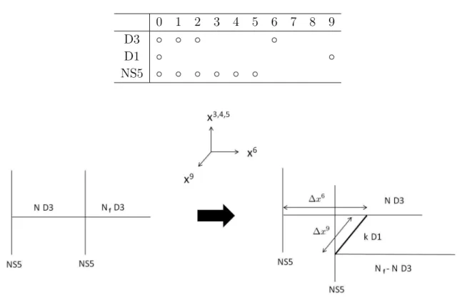
Next let us consider the moduli space using a D-branes system.¹ According to [51], we can obtain the N = 4 U(N) Yang-Mills-Higgs theory using N D3-branes stretched between two NS5-branes as the table below and the left picture of the Fig.2.3. In order to give the hypermultiplets, we connect N semi-infinite D3-branes to the right-hand NS5-brane. In the box, ◦ denotes a stretched direction.

1Although we consider the vortex moduli space using a D-brane system here, it also turns out that they are constructed in a purely field theoretic manner [50].

(20)

0 1 2 3 4 5 6 7 8 9

D3 _{◦ ◦ ◦} _◦

D1 _◦ _◦

NS5 ◦ ◦ ◦ ◦ ◦ ◦

Figure 2.3: Brane construction of the 3d N = 4 SQCD and vortex solution

Furthermore we move one NS5-brane to x⁹ direction, which induces a nonzero FI parameter. Since the D3-branes cannot tilt into the x⁹ direction to preserve the supersymmetry, only N of the Nf D3-branes can end on the N D3-branes according to the S-rule [51]. Fi- nally, the configuration are drawn in the right picture of the Fig.2.3 (without D1-branes). The gauge coupling and FI parameter in the system are given by the following relations,

1 g²_YM ^∼

∆x⁶ gs

, ζ _∼ ^∆x

9

gsl²_s^, ^(2.4.8)

where gs is the string coupling and ls =^√α^′ is string length scale.

Here how is the vortex configuration? In fact the k vortex solution is realized as the k D1-branes stretched along the x⁹ direction between the right-hand NS5 and N D3-branes in the right picture of the Fig.2.3. The D1-branes are identified as unique BPS-branes with the correct mass of the vortex (2.4.5) in this situation.

Let us read off the low energy effective theory on the D1-branes. First this configuration breaks 1/2 of the supersymmetry, so it would be a one-dimensional quantum mechanics with N = (2, 2) type supersymmetry. Since one end of the D1-branes ends on the NS5-brane, the fluctuations of the (x⁶, x⁷, x⁸, x⁹) directions are fixed. Then when we consider massless modes on the D1-branes, the fluctuations of the (x⁰) is a one-dimensional

(21)

U (k) gauge field At, and the ones of the (x³, x⁴, x⁵) are three adjoint scalar fields σ^r (r = 1, 2, 3), which combine into a U (k) vector multiplet. The ones of the (x¹, x²) are also adjoint scalar fields, which correspond to adjoint chiral multiplet. We denote the complex scalar field as Z. Massless modes from open strings which end on the D1 and N D3-branes become N fundamental chiral multiplets [52, 53]. We denote the complex scalar fields as ϕi (i = 1,· · · , N). Also massless modes from open string which end on the D1 and (Nf− N) D3-branes are (N^f− N) anti-fundamental chiral multiplets. We denote the complex scalar field as ˜ϕi^′ (i^′ = N + 1,_{· · · , N}f). Summarizing them, the theory, which describes the vortex, consists of the following set of supermultiplets in one dimension:

• U(k) vector multiplet: (A^t^{, σ}^r^), r = 1, 2, 3,

• an adjoint chiral multiplet: Z ,

• N fundamental chiral multiplets: ϕⁱ^, ^{i = 1,}· · · , N,

• Nf − N anti-fundamental chiral multiplets: ˜^ϕi^′, i^′ = N + 1,_{· · · , N}f , The bosonic part of the Lagrangian is

Lvortex

bos⁼^−Tr

[ ₁ 2e²^D^t^σ

r_D

t^σ^r^{+ D}t^Z^†^Dt^{Z +}

_{[Z, σ}^r_]²₊ ¹ 2e²^[σ

r_{, σ}s_]2 ^]

−D^t^ϕ^†^D^t^ϕ− D^t^ϕ^˜^†^D^t^ϕ^˜− ϕ^†i^ϕⁱ^σ^r^σ^r− Tr^{[ e}

2

2^{([Z, Z}

†_{] + ϕϕ}†_{− ˜}_ϕ†_ϕ_˜_{− r · 1l} k)² ^],

(2.4.9) where we omitted the flavor indices. Then the gauge coupling and FI parameter of this theory are also determined by

1 e² ^∼

l²_s∆x⁹ gs

, r_∼ ^∆x

6

gs

. (2.4.10)

Note that the FI parameter r is related with the gauge coupling gYM in the 3d _{N = 4} theory: r_{∼ 1/g}_YM² .

The global symmetry of this theory is SU (2)R_{× U(1)}F _{× S}

[U (N )_{× U(N}f _{− N)}

], (2.4.11)

where SU (2)R is an R-symmetry which rotates the three scalar fields σ^r of the vector multiplet, U (1)F is a flavor symmetry which rotates the phase of Z, and S[U (N )_× U (Nf − N)] are flavor symmetries of ϕi and ˜ϕi^′ respectively.

Then the condition for the vacuum is

[Z, Z^†] + ϕϕ^†_{− ˜}ϕ^†ϕ^˜_{− r · 1l}k= 0, (2.4.12)

(22)

so the moduli space is

Mk,(N,Nf) =^{(ϕ, ˜ϕ, Z)

[Z, Z^†^{] + ϕϕ}^†− ˜^ϕ^†^{ϕ = r}^˜ · 1lk

}

/U (k). (2.4.13) The degrees of freedom for this moduli space are

dimR(_Mk,(N,Nf)) = 2^{kN + k(Nf − N) + k²^}− k²− k² ^{= 2kN}f, (2.4.14) which equal that of the vortex moduli space which is obtained by the index theorem.[47]

Vortices in 3d N = 2 theories

Let us considerN = 2 U(N) theory with Nf fundamental and ˜Nf anti-fundamental chiral multiplets with the FI term (ζ > 0) [43]. Then the bosonic part of the Lagrangian is

L^bos ⁼ −_g₂¹

YM

Tr^{( 1} 4^F^µν^F

µν₊ ¹

2^D^µ^σD

µ_σ ⁾

− D^µ^ϕ^†^D^µ^ϕ− D^µ^ϕ^˜^β^D^µ^ϕ^˜^†

−ϕ^†^σ²^{ϕ + ˜}^ϕσ²^ϕ^˜^†− Tr^{[ g}

YM2

2 (

ϕ^†ϕ_{− ˜}ϕ ˜ϕ^†₋ ^ζ 2π

)2 ]

, (2.4.15)

where we omit the flavor indices. Here we have a special vacuum with ϕ_{̸= 0 and ˜}ϕ = 0

2. Up to Weyl permutations, we can choose the vacuum as

ϕai=

√ ζ

2π^δ^ai^, ^{σ = ˜}^{ϕ = ϕ}ⁱ^′ ^{= 0,} ^(2.4.16) (a = 1,· · · , N, i = 1, · · · , N, i^′ ^{= N + 1,}· · · , Nf). (2.4.17) In this vacuum, we can show that there also exist half BPS vortex solutions in the same way as we did above.

As we have seen in the brane construction in N = 4 theory, we also expect that the vortex moduli space is characterized by a certain one-dimensional supersymmetric theory. In particular, the authors in [54] have analyzed a half BPS vortex in a supersymmetric theories with four supercharges, and then found that the vortex solutions preserve chiral N = (0, 2) type supersymmetries, rather than N = (1, 1).

Then what is a vortex moduli space for the 3d N = 2 U(N) theory with N^f ^fundamental and ˜Nf anti-fundamental chiral multiplets? Using an analogy of the brane construction in 3d N = 4, we expect that the moduli space is described by the following set of supermultiplets:³

2 If we consider a massive theory, ˜ϕ vanishes for ζ > 0 and generic masses in the vacuum.

3We summarize our notations in appendix D.

(23)

• U(k) vector multiplet: (A^t^{, φ),}

• an adjoint chiral multiplet: B,

• N fundamental chiral multiplets: Iⁱ^{, i = 1,}· · · N,

• Nf − N anti-fundamental chiral multiplets: J^j^, ^{j = N + 1,}· · · , Nf^,

• ˜^N^f fundamental Fermi multiplets: F^p, p = 1,_{· · · , ˜}Nf,

where we have displayed only the bosonic fields of the multiplets, respectively. Note that the contributions of the anti-fundamental matters in three dimensions are characterized by the Fermi multiplets. In fact, we find that the moduli space of this theory is

M^kN,Nf ⁼

{(B, I, J)_{[B, B}^†] + I ¯I_{− ¯}JJ = r_{· 1l}k

}/U (k), (2.4.18)

where r is an FI parameter of this one-dimensional theory. We also find that the degrees of freedom for the moduli space match those of the 3d N = 2 vortex, and the global symmetries are also the same on both side. For example, in two dimensions, it turns out that a gauged matrix model obtained as a dimensional reduction of the above contents can describe a vortex moduli space in 2d N = (2, 2) U(N) theory with N^f fundamental and ˜Nf anti-fundamental chiral multiplets [34].

(24)

Chapter 3 Localization and supersymmetry on

a curved space

3.1 Localization

Supersymmetric localization principle

First let us see that the path integral is reduced to that only over the BPS sector when we consider any supersymmetric observable, along [55] (See also [56]). We consider some expectation value^⟨_O^⟩on the field spaceF, and suppose that the theory and the operator O have a certain symmetry G. Furthermore we assume that G acts freely on F, i.e. there is no fixed point on F. Then, we have a fibration F → F/G. Integrating over the fiber, we obtain

⟨O^⟩ ⁼

∫

F^{O e}

−S _{= vol(G)}_·

∫

F/G^{O e}

−S_. _(3.1.1)

Next we suppose that G is a fermionic symmetry. Then the corresponding volume for the fermionic variable θ is _∫

dθ _{· 1 = 0.} (3.1.2)

That is to say that the contribution vanishes. However, if we consider the case of supersymmetry Q, it cannot act freely. Note that the fixed point set of Q is described by

F^BPS⁼{[X] ∈ F ∀Q(bosons) = 0, ∀Q(fermions) = 0}. ^(3.1.3) Then with this notation, Q acts freely on F \ FBPS. So for this quotient space we find that the contribution vanishes. Therefore the path integral reduces to that only over the BPS sector when we consider any supersymmetric observables.

(25)

Deformation of the path integral

In the above we have seen that a supersymmetric path integral can reduce to just an integral over the BPS configurations. Furthermore we can constrain the configuration of the supersymmetric path integral. First let’s consider a partiton funciton of a supersymmetric theory,

Z =

∫

DΦ e^−S[Φ]^, ^(3.1.4)

where Φ is a set of fields and we assume thatQS = 0 and Q(DΦ) = 0 for supercharge Q. Here we perform the following deformation as for some parameter t and a certain function V [Φ],

Z(t) =

∫

DΦ e⁻

(S[Φ]+tQV [Φ]⁾_, _(3.1.5)

where we assume that t≥ 0 and QV [Φ] ≥ 0 for positive semi-difiniteness, and moreover Q²V = 0. We note that Z(t) reproduces original partition function in the case t = 0. Then we readily find that Z(t) is independent of t since

d

dt^{Z(t) =}

∫

DΦ QV e⁻

(S[Φ]+tQV [Φ]⁾ ₌^∫ _{DΦ Q}⁽_{V e}−⁽S[Φ]+tQV [Φ]⁾⁾= 0, (3.1.6)

where we used the above assumptions, and ignored the boundary contributions. From the above,

Z = Z(0) = Z(t) = Z(_{∞) = lim}

t→∞

∫

DΦ e⁻

(S[Φ]+tQV [Φ]⁾_, _(3.1.7)

so the path integral can result in just a problem of calculating one-loop around the configurations such that QV = 0. In the same way we can apply the same argument for any Q invariant observables. From this discussion, if we take V =^∑all fermions⁽Qψⁱ⁾^†^ψⁱ^{, the path} integral becomes a problem of calculating the one-loop around the BPS configurations.

In conclusion, we find that for any supersymmetric observable such that _{QO[Φ] = 0,}

⟨O^⟩ ^{= lim}

t→∞

∫

F∗

DΦ∗O[Φ∗^{] e}⁻

(S[Φ∗]+tQV [Φ∗]⁾

, for_F_∗ =_{Φ_∗ _{∈ F | F}BPS ∩ QV [Φ∗^{] = 0}},

=

∫

F∗

DΦ∗O[Φ∗^{] e}^−S[Φ^∗^]

1 Sdet^[^δ²_δΦ^S[Φ2^∗^]

∗

] . (3.1.8)

That is to say the infinite dimensional integral can reduce to just the integral over_F_∗, and the result can be exact if the second fluctuations around the classical fields are evaluated. Note that we need a special off-shell symmetry to satisfy one of the above conditions Q²^{V = 0.}

(26)

Figure 3.1: Localized configration in whole field space

Example: Poincar _´ e-Hopf theorem

As an application let us consider the Poincar´e-Hopf theorem along [57]. Let M be a 2n-dimensional Riemannian manifold with metric gµν, vielbein e^a_µ, and let V be a vector field on M . We can consider the following supercoordinates on the tangent bundle,

(x^µ, ψ^µ), (B_µ, ¯ψ_µ), µ = 1, 2,· · · , 2n, ^(3.1.9) where x^µ is a coordinate on the base tangent space, and ψ^µ is the fiber coordinate associated with the following fermionic symmetry,

δx^µ = ψ^µ, δ ¯ψµ= Bµ,

δψ^µ= 0, δB_µ= 0, (3.1.10)

where (Bµ, ¯ψµ) is a just pair of auxiliary variables. We can verify that δ² = 0 immediately. In this setup let us consider a partition function.

Z(t) = ¹

(2π)²ⁿ

∫

d²ⁿx d²ⁿψ d²ⁿψ d^¯ ²ⁿB e^−S(t), (3.1.11) where

S(t) = δ^{[ 1} 2^ψ^¯^µ

(B^µ+ 2itV^µ+ g^µτΓ_{τ ν}^σ ψ^¯_σψ^ν^)]. (3.1.12)

From the above discussion S(t) is independent of the parameter t since it is δ-exact. Integrating Bµ out, we have

Z(t) =

√_g (2π)ⁿ

∫

dxdψd ¯ψ exp^[₋^{( t}

2

2^V^µ^V

µ_{− it(∇}

µV^ν) ¯ψνψ^µ₋¹ 4^R

µνστ^ψ^¯µψ^¯νψ^σψ^τ^)]. (3.1.13) Since Z(t) is independent of t, we first consider the case of t = 0,

Z(0) = ¹

(2π)ⁿ

∫ √g dx dψ d ¯ψ exp^{[ 1} 4^R

µν

στ^ψ^¯^µ^ψ^¯^ν^ψ^σ^ψ^τ

]

(27)

= ¹ (2π)ⁿ

∫ √_{g dx Pf(R)}

=

∫

M

e(M ) = χ(M ), (3.1.14)

where e(X) and χ(X) are the Euler class and Euler characteristic, respectively. In the last line we used the Gauss-Bonnet theorem. Next we evaluate the case of t = _{∞. We} assume that V has isolated and simple zeros p_k, V (p_k) = 0. Since the contribution for V = 0 is dominant, we expand V^µ around the zero, for ξ^µ= x^µ_{− p}^µ_k,

V^µ(x) = ∂_νV^µ(p_k)ξ^ν + ¹ 2^∂^ν^∂^ρ^V

µ_(p

k^)ξ^ν^ξ^ρ⁺· · · . ^(3.1.15) Also we rescale as

ξ _{→ t}⁻¹ξ, ψ _{→ t}^−1/2ψ, χ_{→ t}^−1/2χ. (3.1.16) Note that the measure is invariant for this rescaling. In the limit t→ ∞, we find

Z(_{∞) =} ^∑

pk

1 (2π)ⁿ

∫

M

√g dξ dψ d ¯ψ exp^[₋ ¹

2^g^µν^∂^ρ^V

ν_(p

k⁾· ∂σ^V^µ^(pk^)ξ^ρ^ξ^σ ^{+ i∂}µ^V^ν^(pk^{) ¯}^ψν^ψ^µ

]

= ^∑

pk

det(∂µV^ν(pk))

√det(∂µV^ν(pk))²^. ^(3.1.17)

Thus, from (3.1.14) and (3.1.17), we obtain the Poincar´e-Hopf theorem, χ(M ) =^∑

pk

det(∂µV^ν(pk))

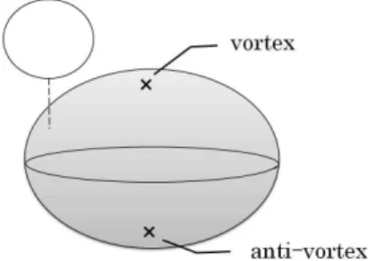
| det(∂^µ^V^ν^(p^k⁾⁾|^. ^(3.1.18) For example let’s consider the two-sphere case. Here we set V_i = _−y_i_∂x^∂

i ^{+ x}ⁱ

∂

∂yi ^{(i =}

N, S) where N and S denote the north and south patches respectively. Then V has two isolated and simple zeros at the north(xN = yN = 0) and south(xS = yS = 0) poles. Then,

det(∂µV^ν) = det^(∂^x^V

x _∂ x^V^y

∂yV^x ∂yV^y )

= 1. (3.1.19)

Therefore we can obtain the well-known result,

χ(S²) = 2. (3.1.20)

(28)

Figure 3.2: Euler characteristic on S²

3.2 Rigid supersymmetry on a curved space

In the above discussion there is a problem, that is the IR-divergence caused by infinity of the space. Although we have to consider a theory with IR-cutoff which preserves symmetries, it is more convenient to consider a theory on a compact space, which provides the IR-cutoff automatically. In this section we consider the supersymmetric theory on a curved space. Note that we consider Euclidean theories in the following.

Construction of supersymmetry on a curved space

Let us present the outline of the construction of the supersymmetric theory on a curved space along [12] (see also [56]). We should add to the well-known flat-space SUSY La- grangian some appropriate corrections corresponding to the curved spaceM we consider. Given the Lagrangian and supersymmetry transformation on the flat space, and the characteristic scale of _{M as L}⁽⁰⁾_M =_LR^d, δ⁽⁰⁾ = δR^d and r, then we would obtain a Lagragian and a supersymmetric transformation on M in as follows,

LM ⁼L⁽⁰⁾_M ^{+ δ}LM ⁼

∑∞ n=0

1 rⁿ^L

(n)

M^, ^(3.2.1)

δ_M =

∑∞ n=0

1 rⁿ^δ

(n)_, _(3.2.2)

where we have to determine the each correction term order by order to preserve the supersymmetry and close the algebra. At first sight they seem to be an infinite summation, but since r has an inverse mass dimension, we do not need to consider irrelevant operators at UV similarly to the renormalization group argument. However, since this idea depends on the space, we instead consider the idea of [12]. This idea provides us with the systematic construction of a supersymmetric theory on a curved space, and as a result we can find

(29)

that the above corrections in the Lagrangian terminate at second order, and those in the supersymmetry transformation terminate at first order, which are consistent with the above idea.

Let us give the outline. First we consider an appropriate supergravty theory, and take a rigid limit, i.e. taking the Newton constant G_N to zero (Planck mass M_P to infinity), while keeping the metric on M at the same time. Then the gravity decouples from the theory, and we can obtain a supersymmetric theory on the curved space M, where the metric and the other auxiliary fields in the gravity multiplet become just backgrounds. Although we do not have to consider their equations of motions, we should require the conditions that the background is also supersymmetric,

Ψ^α_µ= 0, δΨ^α_µ = 0, (3.2.3)

where Ψ is gravitino and δΨ implies the transformation in the supergravity theory. The conditions correspond to Killing spinor equations, where the spinors respect the supersymmetries on _M.

Minimal coupling with supergravity multiplet

If we know the corresponding supergravity theory, we should apply the above discussion. However, even if we do not know such a supergravity theory, we can still construct such a supersymmetric theory on a curved space. First recall the prescription of coupling a theory with a gauge field.

We should replace the ordinary derivative with a gauge covariant derivative: ∂µ → Dµ= ∂µ− iAµ. The minimally coupled Lagrangian is written as

L(Φ, DΦ) = L(Φ, ∂Φ) − j^µ^Aµ⁺O(A²^), ^(3.2.4) where j^µ is a conserved current for the original global symmetry, and also written by

j^µ=₋ ^∂^L

∂Aµ

A=0^. ^(3.2.5)

If we want to obtain a dynamical gauge theory, we should add the Yang-Mills kinetic term. We can extend this idea to spacetime symmetries. The associated current with the Poincar´e symmetry is the energy-momentum tensor T^µν. The coupled theory is obtained by replacing the flat metric ηµν and the ordinary derivative with a curved metric gµν = η_µν _{− 2h}_µν and the general covariant derivative _∇_µ in the same way. The minimally coupled Lagrangian is

L = L⁽⁰⁾− T^µν^h^µν ⁺O(h²^). ^(3.2.6)

本文 Thesis 総合研究大学院大学学術情報リポジトリ A1754本文

Higgs branch localization of

three-dimensional

supersymmetric gauge theories

Masashi Fujitsuka

Doctor of Philosophy

Department of Particle and Nuclear Physics

School of High Energy Accelerator Science

The Graduate University for Advanced Studies

2014

Abstract

Acknowledgments

Contents

Chapter 1

Introduction

Chapter 2

Supersymmetric gauge theories

2.1 3d N = 2 supersymmetric gauge theory

Euclidean supersymmetry

2.2 Level shift and parity anomaly

2.3 Supersymmetric vacua

2.4 Dynamics of vortices

Vortex solutions and brane construction in 3d N = 4 theories

Vortices in 3d N = 2 theories

Chapter 3

Localization and supersymmetry on

a curved space

3.1 Localization

Supersymmetric localization principle

Deformation of the path integral

Example: Poincar ´ e-Hopf theorem

3.2 Rigid supersymmetry on a curved space

Construction of supersymmetry on a curved space

Minimal coupling with supergravity multiplet

Example: Poincar _´ e-Hopf theorem