本文総合研究大学院大学学術情報リポジトリ甲1420 本文

(1)

Statistical Estimation of Phase Response Curves

Ken Nakae

DOCTOR OF PHILOSOPHY

Department of Statistical Science

School of Multidisciplinary Science

The Graduate University for Advanced Studies

2010 (School Year)

(2)

(3)

Abstract

Phase response curve (PRC) describes the response of an oscillator to external perturbation; it is useful to predict and understand synchronized dynamics of oscillators. In recent years, neuroscientists have focused on neurons’ PRCs, and measured them experimentally. This originates from the leading hypotheses that the synchronization of neurons has a functional meaning in the brain.

In this thesis, we propose two statistical methods for estimating PRCs from data; it allows for the correlation of errors in explanatory and response variables of the PRC. This correlation is neglected in previous studies.

The first method is implemented with a replica exchange Monte Carlo technique; this avoids local minima and enables efficient calculation of posterior averages. A test with artificial data generated by noisy Morris-Lecar equations shows that, in terms of accuracy, this method outperforms conventional regression that ignores errors in the explanatory variable. Experimental data from the pyramidal cells in the rat motor cortex is also analyzed; a case is found where the result with the first method is considerably different from that obtained by conventional regression.

The second method is developed using a transformation that mixes the variables; it effectively removes the correlation. The computation time of this method is considerably less than that of the first method. The same test using the noisy Morris-Lecar equations shows that the second method also outperforms than convectional regression in terms of accuracy.

(4)

(5)

Acknowledgment

I am deeply grateful to my supervisor Associate Professor Yukito Iba. I would like to express my gratitude to Associate Professor Toshio Aoyagi, who was my supervisor of my master course in Kyoto University.

I am indebt to Professor Tomoyuki Higuchi and Professor Kenji Fukumizu whose comments made enormous contribution to this thesis. Professor Tomoki Fukai in RIKEN gave insightful comments, and encouraged me to apply the method in this thesis to experimental data. Dr. Tsubo Yasuhiro in RIKEN provided the experimental data. Discussion with him has been interesting for me.

I have had the encouragement of Professor Takashi Tsuchiya in National Graduate In- stitute for Policy Studies, Professor Satoshi Kuriki, Professor Hiroe Tsubaki and Associate Professor Genta Ueno in the Institute of Statistical Mathematics. Special thanks to Profes- sor Nobuhisa Kashiwagi in the Institute of Statistical Mathematics and Assistant Professor Hayato Chiba in Kyushu University, who give important comments in my research.

I would like to express my gratitude to President Genshiro Kitagawa in the Research Organization of Information and Systems, Associate Professor Toshio Ohnishi in Kyushu University, Dr. Hai-Yen Siew in Meiji University, Professor Emeritus Yoshiaki Itoh, As- sociate Professor Yoichi Nishiyama, Assistant Professor Shogo Kato, Dr. Xiaoling Dou and Dr. Ushio Tanaka in the Institute of Statistical Mathematics. We had a talk in Indian Statistical Institute; this made me decide to be a researcher.

I want to thank my colleagues in Kyoto University and in the Graduate University for Advanced Studies. I especially thank my friends Dr. Keisuke Ota and Mr. Kaiichiro Ota, who and I often discuss my research. My heartfelt appreciation goes to my family, who support me in the doctor course.

This research was supported by an allocation of computing resources of HP XC4000

(6)

6

and Fujitsu PRIMERGY RX200S5 from the Institute of Statistical Mathematics.

(7)

Overview of this thesis

This thesis is divided into 3 parts and consists of 10 chapters. Part I (Chap. 1–4) provides the background and motivation of this thesis. In part II (Chap. 5–7), we propose a Bayesian method for estimating PRCs, where we consider a correlation between the explanatory and response variables. This method is implemented with replica exchange Monte Carlo methods. In part III (Chap. 8–10), we propose another statistical method, which also consider the correlation. A transformation that removes the correlation plays an essential role in this part. In Chap. 10, we summarize this thesis and discuss future problems.

The details of each part are as follows:

Part I In Chap. 1, we briefly discuss motivations of this thesis and concepts of synchronization and phase response curve. The detail of the concept is discussed in Chap. 2. In Chap. 3, we review methods for estimating PRCs including that proposed in my master thesis. We discuss drawbacks of these methods, and discuss our approach of this thesis. In Chap. 4, we briefly discuss a Bayesian framework used in this thesis, and introduce Metropolis-Hastings methods and replica exchange Monte Carlo methods used in part II.

Part II In Chap. 5, we derive a Bayesian model, which describes a correlation between errors in PRC explanatory and response variables. In Chap. 6, we propose a Bayesian method for estimating PRCs using replica exchange Monte Carlo methods. In Chap. 7, this proposed method is tested with artificial data generated by noisy Morris-Lecar equations. We compare the method with conventional regression in terms of accuracy for the data. We also analyze experimental data from the pyramidal cells in the rat motor cortex.

Part III In Chap. 8, we propose a statistical method using a data transformation that mixes the PRC explanatory and response variables. This method is based on a modification of the model in part II. In Chap. 9, the method in part III is compared with the method in II and conventional regression in terms of accuracy and computation time. In Chap. 10,

7

(8)

8

summary and future problems are presented.

(9)

Background and motivation

13

(14)

14

(15)

Chapter 1

Introduction

1.1 Synchronization

Synchronization is observed everywhere in nature [Pikovsky et al., 2002, Strogatz, 2004]. For example, beating of the heart is a result of the synchronization of the cell activities of the heart muscles [Reemtsen and Rueckmann, 1983]. Fireflies in an area of Southeast Asia flash periodically and simultaneously [Smith, 1935, Buck and Buck, 1968, Ermentrout and Rinzel, 1984], which is first reported by E. Kaempfer in 18-th century. Synchronizations are also observed in chirps of the snowy tree crickets [Walker, 1969] and in croaking of the neighboring two tree frogs [Aihara et al., 2007, Aihara, 2009]. We encounter synchronization phenomena in biology [Aschoff et al., 1982, Dano et al., 1999, Elowitz and Leibler, 2000], in chemistry [Toth et al., 2006, Mikhailov and Showalter, 2006], and in physics [Si- monet et al., 1994, Pantaleone, 2002, Eckhardt et al., 2007, Kitahata et al., 2009].

In the brain, we also observe synchronization between neurons and its result [Salinas and Sejnowski, 2001, Varela et al., 2001]. For example, gamma frequency oscillations observed in the local field potential of the mammalian olfactory bulbs is considered to be the result of synchronous activities of the neurons [Adrian, 1950, Freeman, 1972, Schoppa, 2006]. A periodic activity of electroencephalogram is also the result of the synchronization [Eccles, 1951, Singer, 1999, Whittingstall and Logothetis, 2009]. Epilepsy is caused by an abnormal synchronization between neurons [Engel et al., 2007, Lehnertz et al., 2009]. In these examples, oscillatory phenomena are often observed as the result of the synchronization of neurons.

15

(16)

16 CHAPTER 1. INTRODUCTION

In recent years, we have directly observed the synchronization between neurons because of the developments of systems for recoding the neural population [Nicolelis et al., 1999]. For example, activities of neurons are measured by multi electrodes systems [Thomas et al., 1972, Taketani et al., 2006], calcium imaging [Grynkiewicz et al., 1985, Stosiek et al., 2003], and voltage sensitive dye imaging [Cohen and Salzberg, 1978, Zochowski et al., 2000] of the neurons. Using them, the synchronization are experimentally detected in various areas of the brain: for example, motor cortex [Riehle et al., 1997, Baker et al., 2001], somatosensory cortex [Steinmetz et al., 2000, Roy et al., 2001], visual cortex [Fries et al., 2001, Freiwald et al., 2001] and basal ganglia [Goldberg et al., 2004].

Neuroscientists have been focusing functions of synchronization in the brain [Buzs´aki, 2006]. This is because some hypotheses are proposed that the synchronization is essential for understanding information processing of the brain [Malsburg and Schneider, 1986, Gray and Singer, 1989, Fries, 2005, Engel et al., 2001, Hopfield and Brody, 2001, Aoki and Aoyagi, 2007]. These hypotheses argue that coherence in neural activities induced by synchronization is not a side effect but essential for understanding brain functions.

Here, we briefly explain one of the hypotheses proposed by Malsburg and Schneider [1986] that the synchronization is closely related to the “binding problem” of cognitive neuroscience. To understand the binding problem and the hypothesis, we present an example where a person looks a brown disc as shown in Fig. 1.1. According to the studies in neuroscience [Gazzaniga, 2004], it is known that the information of the shape and the color of the disc is distributed in different regions in visual cortex of the brain. Through an unknown information processing, the person bind the information of the shape and the color, and recognize “This is a brown disc”. In this example, the binding problem is a question: What is the unknown information processing? Gray and Singer [1989] try to answer the question through the hypothesis that binding of information occurs because of the synchronizations between the spikes of neurons in the corresponding areas. Many researchers have tried to investigate the binding problem and this hypothesis from various aspects [Revonsuo and Newman, 1999, Thiele and Stoner, 2003, Bartels and Zeki, 2006, Dong et al., 2008].

(17)

1.2. PHASE RESPONSE CURVES AND COUPLED PHASE OSCILLATORS 17

observation

color

shape

This is a brown disc. _spikes

synchronization

recognition

Figure 1.1: A example of the binding problem and the hypothesis proposed by Malsburg and Schnei- der [1986].

1.2 Phase response curves and coupled phase oscillators

Phase response curves

To deal with synchronization from the theoretical viewpoint, Kuramoto [1984] developed a theory based on phase reduction from interacting nonlinear oscillators to “coupled phase oscillators”; see also [Malkin, 1949, 1959, Winfree, 1967, 2001, Kopell and Ermentrout, 1990, Hansel et al., 1995, Ermentrout, 1996, Izhikevich, 2007, Kuramoto and Kawamura, 2010] and recent surveys [Strogatz, 2000, Acebron et al., 2005]. A key concept of this theory is a phase response curve (PRC), which describes the response of an isolated oscillator to external perturbations. The PRCs are usually defined from the viewpoint of the dynamical systems; here, we assume that the oscillator has a stable limit cycle. This means that no closed orbit exists near the limit cycle, and it attracts all neighboring trajectories.

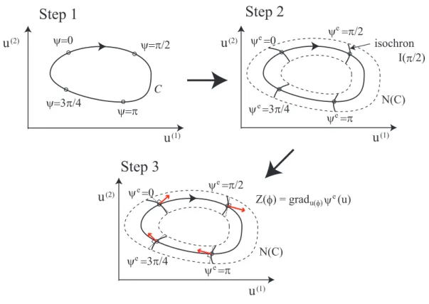
Here, we explain an definition of the PRCs, where we assume ad-dimensional dynamical system u(t) has a stable limit cycle C as shown in the upper-left panel of Fig. 1.2. The procedure consists of the following three steps:

1. We define a smooth and bijective function on the limit cycle ψ : C _{→ S}¹, which corresponds to a phase variable from0 to 2π of the oscillator, as shown in the upper- left panel.

(18)

2. Under regularity conditions [Coddington and Levinson, 1955, Guckenheimer, 1975], the domain of ψ is appropriately ¹ extended to a neighborhood N (C) of the limit cycle; i.e. the extended function ψê : N (C) _{→ S}¹ satisfies ψê_|C = ψ. The d_{− 1} dimensional manifoldI(ϕ) ={u ∈ N(C)|ψê^{(u) = ϕ}} is called an isochron, which is shown as the curve of the upper-right panel.

3. Finally, we obtain the phase response curves (PRCs) Z(ϕ) = gradu_(φ)∈Cψ^e(u), which is ad-dimensional periodic vector function. The right side of this equation means a normal vector at u(ϕ) := ψ⁻¹(ϕ) on the isochron I(ϕ). The red arrows in the lower panel show the normal vectors.

Thed-dimensional dynamics of the oscillator can be reduced to a one-dimensional dynamics of the phase variableϕ where phase shifts by external perturbations are described by the PRCs. In this thesis, we call this reduction “phase reduction of the oscillator”.

Another definition of phase response curves

Here, we explain an operational definition of the PRCs, which is more intuitive and useful for understanding experiments. Its correspondence to the definition based on phase description of the dynamical systems is explained in the next section.

We define PRC Z(ϕ) of a nonlinear oscillator from an operational viewpoint. PRC Z(ϕ) = (Z⁽¹⁾(ϕ), . . . , Z^(d)(ϕ)) is a periodic d-dimensional vector function in the domain [0, 2π), when the dynamical system of the oscillator has d-dimensional state.

As an example of the nonlinear oscillator, we consider a neuron, whose activity is periodic. The state of the neuron has various components, which correspond to the activities of the voltage, the potassium channel, the sodium channel and so on. Here, we operationally define the voltage component of PRC Z(ϕ); it is denoted by Z(ϕ). This is because other components of PRC can be defined in the same manner, and the voltage component of the PRC gives sufficient information to analyze the synchronization of neurons. The latter reason will be explained in Sec. 2.2

We assume that the activity of a neuron is periodic and the period isT . The solid curve in the left panel of Fig. 1.3 represents a time-series of the voltage for the neuron. We

1In an asymptotic sense (t → ∞), we can identify a point u^′on the limit cycle as points at which values of ψ^eare equal to the phase of the point u^′; the set of the identifiable points is an d − 1-dimensional manifold “isochron”, which is shown as the curves in the upper-right panel.

(19)

ψ=0 _ψ=π/2

ψ=3π/4 ψ=π

ψ =0 ^{ψ =π/2}

ψ =π ψ =3π/4

C

N(C)

ψ =0 ^{ψ =π/2}

ψ =π

ψ =3π/4 ^N(C)

Z(φ) = grad ψ (u)

e

e e

e

u(φ) e

u⁽¹⁾ u⁽¹⁾

u⁽¹⁾

u⁽²⁾ u⁽²⁾

u⁽²⁾

I(π/2) isochron

Step 1 ^{Step 2}

Step 3

Figure 1.2: Three steps of defining the PRCs ofd = 2 dimensional dynamical system.

consider a set of trials indexed by i. The neuron is assumed to fire at the origin t = 0. For theith trial, a perturbation is added at time t = ti. The neuron then fires again at time t = T_i^′ as shown by the dotted curve in the Fig. 1.3. We repeat this procedure a number of times and plot the points(ϕi, Zi), i = 1,· · · , n, defined by

ϕi = 2π^tⁱ

T^, ^Zⁱ ^{= 2π}

T _{− T}_i^′

T ^. ^(1.1)

A smooth and periodic curveZ(ϕ) interpolating these points in the domain [0, 2π) is the voltage component of the PRC of the neuron. The example of the curve is shown by the solid curve in the right panel of Fig. 1.3.

(20)

voltage

current

0 2π

0

Figure 1.3: Measurement of a phase response curve. A trial with a perturbation att = t_iis illustrated in the left panel. The solid curve indicates the voltage for the neuron without perturbation, while the dotted curve indicates that with perturbation. Each point(φ_i, Z_i) in the right panel corresponds to a trial with timingt_i. PRC is defined by interpolating these points.

Connection to the definition through dynamical systems

In the previous section, we explain an operational definition of PRC of a nonlinear oscillator. Conventionally, the PRC is defined through phase reduction of the dynamical system of the oscillator. Here, we discuss a correspondence between two definitions of the PRC. Details of the phase reduction can be found in the book [Kuramoto, 1984].

Here, we revisit the phase reduction of the oscillator from the viewpoint of dynamical system. Let us represent the state of the oscillator by the vector u= (u⁽¹⁾, . . . , u^(d))_{∈ R}^m. An equation that describes dynamics of the oscillator is assumed as

du

dt = f (u) + p(t), (1.2)

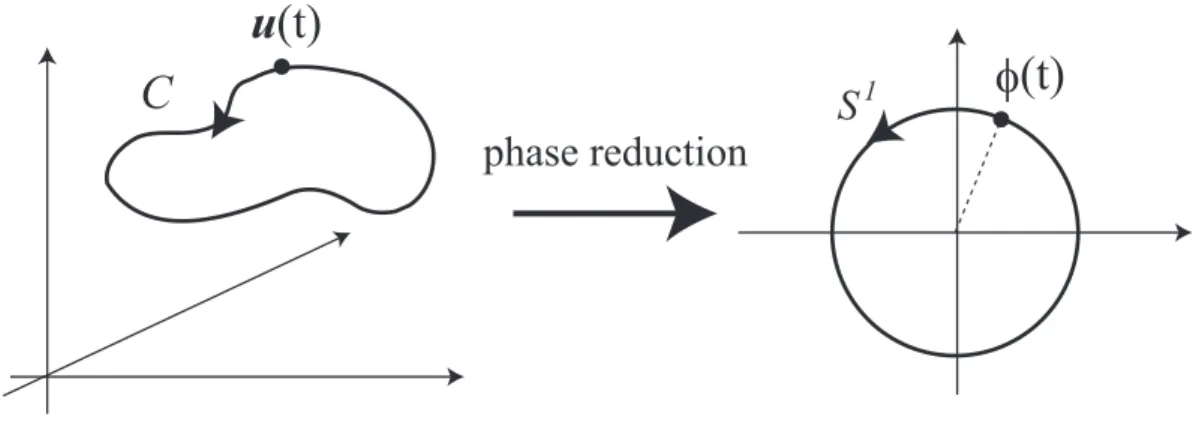
where the vector field f(u) has a stable limit cycle C as shown in the left panel of Fig. 1.4. The vector p(t) = (p⁽¹⁾(t),_{· · · , p}^(d)(t)) represents an external perturbation. When f (u) satisfies regular conditions [Coddington and Levinson, 1955, Guckenheimer, 1975] and

(21)

p(t) is sufficiently small, Eq. (1.2) is reduced to the dynamics dϕ

dt ^{= ω + Z(ϕ)}^{· p(t),} ^(1.3)

where the natural frequency ω is 2π/T and a point on C is indicated by the phase variable ϕ ∈ [0, 2π) [Kuramoto, 1984]. The smooth and periodic vector function Z(ϕ) = (Z⁽¹⁾(ϕ), . . . , Z^(d)(ϕ)) represents a response of the oscillator to the perturbation p(t). As shown in Fig. 1.4, the dynamics of the state u(t) on the limit cycle C is reduced to the dynamics of the angle ϕ(t) of the unit circle. This reduction from Eq.(1.2) to Eq.(1.3) is called the phase reduction of the oscillator.

C _S

¹

u _(t)

φ(t)

phase reduction

Figure 1.4: Phase reduction of a dynamical system that has a limit cycleC.

To show a correspondence to the operational definition, we assume that the first com- ponentu⁽¹⁾of the state is the voltage of the neuron discussed in the previous section. When the perturbation p(t) is added to the first component u⁽¹⁾ only and the functional form of p⁽¹⁾(t) is the Dirac’s delta function δ(t_{− t}i), Eqs. (1.2) and (1.3) correspond to the ex- periment defining PRC Z(ϕ) from the operational viewpoint. Thus, we can identify the function Z⁽¹⁾(ϕ) in Eq. (1.3) with a PRC Z(ϕ) defined operationally. This can be seen by integrating Eq. (1.3) in the regions [0, ti) and [0, Ti). As a result, we derive the two equations

ϕ(t_i) = 2π^tⁱ

T^, ^Z

(1)_(ϕ(t

i^{)) = 2π}

T _{− T}_i^′

T ^, ^(1.4)

which correspond the left and right equations in Eq. (1.1) respectively.

(22)

Coupled phase oscillators

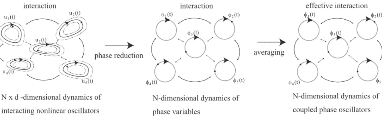
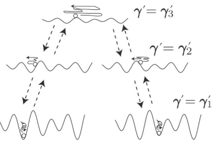
In the theory developed by Kuramoto [1984], we deal with synchronization of the dynamics ofN interacting nonlinear oscillators. Phase reduction of each oscillator reduces the N_×d- dimensional dynamics of all oscillators to that ofN -dimensional dynamics of their phase variables as shown in the left and middle panels of Fig. 1.5.

Coupled phase oscillators are defined through averaging of the interactions and the PRCs in this N -dimensional dynamical system; the average is considered as an effective interaction called a coupling function. Coupled phase oscillators provide a concise description of the original interacting nonlinear oscillators. In Fig. 1.5, we illustrate the above procedure that derives the coupled phase oscillators. Details of the procedure are explained in Chap. 2.

phase reduction interaction

u (t)₁ ^{u (t)}²

u (t)3

u (t)₄

u (t)5

N x d -dimensional dynamics of interacting nonlinear oscillators

interaction

N-dimensional dynamics of phase variables

φ (t)2

φ (t)₁

φ (t)₃

φ (t)4 ^{φ (t)}⁵

averaging

effective interaction

N-dimensional dynamics of coupled phase oscillators

φ (t)₂ φ (t)1

φ (t)3

φ (t)₄ ^{φ (t)}⁵

Figure 1.5: Phase reduction from interacting nonlinear oscillators to coupled phase oscillators.

From a viewpoint of statistical physics, Kuramoto [1975] studied coupled phase oscillators (Kuramoto model) where all coupling functions are the same sine function, and natural frequencies of the oscillators follow a Cauchy distribution. Using an analytical technique, he found a transition from synchrony to asynchrony state of the coupled phase oscillators whenN → ∞. Being motivated by this study, many researcher investigate synchronization properties of various types of coupled phase oscillators and dynamics of coupled phase oscillators [Hansel et al., 1993, Kori and Kuramoto, 2001, Strogatz and Mirollo, 1991, Daido, 1994, 1996, Crawford, 1995, Sakaguchi et al., 1987, Hong et al., 2005, Ichinomiya, 2004, Kuramoto and Battogtokh, 2002].

(23)

1.3. PHASE RESPONSE CURVES IN NEUROSCIENCE 23

These theoretical results refresh scientists for studying synchronization phenomena in biology [Aihara et al., 2007, Aihara, 2009], chemistry [Kiss et al., 2002, Zhai et al., 2004] and physics [Wiesenfeld et al., 1996, Strogatz et al., 2005]. They apply this theory to these phenomena and obtain successful results.

1.3 Phase response curves in neuroscience

Theoretical results

Here, we briefly discuss theoretical results about PRCs of neurons in this section, and show experimental data of the PRCs in the next section.

The PRCs Z(ϕ) of a neuron have many components. For example, Hodgkin-Huxley equations [Hodgkin and Huxley, 1952], which is widely used for a mathematical neuron model, are described as a four-dimensional dynamical system; the components of the state are denoted by the activities of the voltagev, the potassium channel n, and the sodium chan- nelm, h (the details are explained in Appendix. B). Thus, the PRCs has four corresponding componentsZv(ϕ), Zn(ϕ), Zm(ϕ) and Zh(ϕ) as shown in the upper-left, upper-right, lower- left and lower-right panels of Fig. 1.6, respectively.

Many neuroscientists discuss only a voltage component of the PRCs of a neuron. This is because the voltage componentZv(ϕ) of the PRCs gives sufficient information to analyze the synchronization of neurons, as we discuss in Sec. 2.2. This means that the component Zv(ϕ) is an essential representation of the dynamics of the neuron; hereafter, we call it the PRCZ(ϕ) of the neuron.

From theoretical viewpoints, synchronization properties of neurons can be predicted using their PRCsZ(ϕ). According to the study by Hansel et al. [1995], two types of PRCs of neurons are classified:

1. For all phasesϕ ∈ [0, 2π), the value of the PRC Z(ϕ) is positive as shown in the left panel of Fig. 1.7; it is called a type-I PRC.

2. For a phaseϕ ∈ [0, 2π), the value of the PRC is negative as shown in the right panel of Fig. 1.7; it is called a type-II PRC.

They conclude that neurons which have type-II PRCs are easier to synchronize than neurons which have type-I PRCs. This result is supported by these successive studies [Nomura and

(24)

0 2_π

0

φ

Ζ (φ)

_v

0 2_π

0

φ

Ζ (φ)

n

0 2_π

0

Ζ (φ)

_m

φ

⁰ ²^π

0

Ζ (φ)

h

φ

Figure 1.6: PRCs of Hodgkin-Huxley equations.

Aoyagi, 2005, Gal´an et al., 2007a,b, Marella and Ermentrout, 2008, Abouzeid and Ermen- trout, 2009]. Based on the classification Tsubo et al. [2007b] predict the synchronization properties of neurons in rat motor cortex using the PRCs estimated from experimental data. This analysis shows that activities of neurons in the layer II/III of the cortex are easier to synchronize than that in the layer V.

0 2_π

0

φ

Ζ(φ)

₀

0

_φ

2_π

Ζ(φ)

Figure 1.7: Type-I and Type-II PRCs.

(25)

1.4. MOTIVATION OF THIS THESIS 25

PRCs are useful for not only predicting but also understanding synchronization phenomena in neural populations. For example, experimental results by Mainen and Sejnowski [1995] indicates that neurons synchronize when common noises input to them. Such a

“noise induced synchronization” can be explained by the dynamical system based on the PRCs of neurons [Teramae and Fukai, 2008, Lin et al., 2009, Garc´ıa- ´Alvarez et al., 2009]. Experimental data

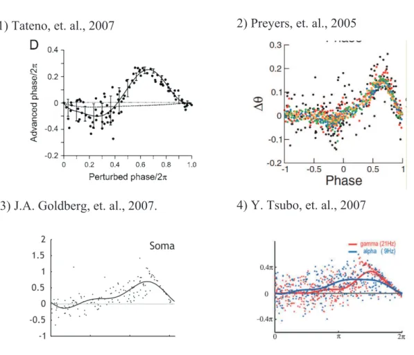
Many researchers have recently tried to estimate neuron’s PRC Z(ϕ) from experimental data in various areas of the brain [Reyes and Fetz, 1993a,b, Dorval et al., 2001, Oprisan et al., 2003, 2004, Gal´an et al., 2005, Gutkin et al., 2005, Lengyel et al., 2005, Netoff et al., 2005a,b, Preyer and Butera, 2005, Ermentrout and Saunders, 2006, Ermentrout et al., 2007, Goldberg et al., 2007, Mancilla et al., 2007, Tateno and Robinson, 2007, Tsubo et al., 2007a, Ota et al., 2009a, Ota, 2010, Phoka et al., 2010]. In Fig. 1.8, we present some examples of the data (the black or colored points) and the estimated PRCs (the black or colored curve). The data in the upper-left and upper-right panels are measured by neurons in rat somatosensory cortex [Tateno and Robinson, 2007] and in the abdominal ganglia of Aplysia californica [Preyer and Butera, 2005], respectively. The data in the lower-left and lower-right panels are measured by neurons in rat neocortex [Goldberg et al., 2007] and in rat motor cortex [Tsubo et al., 2007a], respectively.

In these examples, a sample (x, y) is obtained by adding an external perturbation to a neuron. The explanatory variablex correspond to timing of the perturbation. The response variabley corresponds the difference between neuron’s period and the inter-spike interval when adding the perturbation. Details of the experiments are explained in Chap. 3. Note that all PRCs of Fig. 1.8 are estimated using regression analysis where errors in the response variable are only considered.

1.4 Motivation of this thesis

As shown in these examples, noise in the PRC measurements is often very large, and so- phisticated statistical techniques are necessary for efficient estimation. In Chap. 3, we discuss the following two facts:

• A data point (x, y) whose value x ≥ 2π can exist in experiments.

(26)

2) Preyers, et. al., 2005 1) Tateno, et. al., 2007

3) J.A. Goldberg, et. al., 2007. 4) Y. Tsubo, et. al., 2007

Figure 1.8: Experimental data (black or colored points) and estimated PRCs (black or colored curves).

• All data points are in the region K = {(x, y) ∈ R²|x ≥ 0, x + y ≤ 2π}.

To see these facts, we present experimental data measured in rat motor cortex, which are shown as the points of Fig. 1.9; the data are provided by my coworkers Yasuhiro Tsubo. Actually, a data point(x, y) whose value x≥ 2π exists, and all data points are in the region K shown as the mesh region of Fig. 1.9. In the conventional regression analysis, the data point whose valuex≥ 2π are neglected, because PRC is a periodic in the region [0, 2π).

These facts can be explained by existences of the errors in the PRC explanatory variables and the correlation between errors in the explanatory and response variables, which are discussed in Chap. 3. The role of errors in explanatory variables for regression has been considered in the literature on statistics [Amari and Kawanabe, 1997, Cheng and Ness,

(27)

1.4. MOTIVATION OF THIS THESIS 27

2π

0 response

0 _phase _x ^2π

y

K

Figure 1.9: Experimental data and the regionK ={(x, y) ∈ R²|x ≥ 0, x + y ≤ 2π}.

1999, Berry et al., 2002, Fuller, 2006, Caroll et al., 2006]. The correlation between errors in the explanatory and response variables is also treated in some textbooks, for example, [Cheng and Ness, 1999], but it seems a less known subject; its appearance in the present problem of estimating PRCs will be interesting in terms of statistical science.

This study is devoted to developing two new methods that can deal with these errors and the correlation. In part II, we propose a Bayesian model accounting for them, and estimate PRCs using replica exchange Monte Carlo methods [Hukushima and Nemoto, 1996, Geyer and Thompson, 1995, Iba, 2001]. In part III, the correlation is effectively removed using a transformation that mixes the explanatory and response variables.

Using the proposed methods, we successfully improved the estimation precision for PRCs in examples of simulated data. The method proposed in part II is also applied to experimental data from the pyramidal cells in rat motor cortex.

The proposed methods for PRC estimation are useful for any kind of nonlinear oscillator that permits the phase description. Although our current interest is in applications for brain science, the method can also be used in other fields of biology, chemistry, and physics.

(28)

(29)

Chapter 2

Theory of synchronization

Kuramoto [1984] developed a theory based on collective dynamics of interacting nonlinear oscillators; it explains various examples of the synchronization phenomena. In this chapter, we explain this theory and its application in neuroscience. We first explain dynamics of coupled phase oscillators and analyze the synchronicity of two coupled phase oscillators in Sec. 2.1. An application of the theory to neuroscience discussed in Sec. 2.2.

2.1 Coupled phase oscillators

2.1.1 Phase reduction and averaging of interacting nonlinear oscillators

Coupled phase oscillators are derived from interacting nonlinear oscillators by applying the phase reduction and an averaging technique. Here, the dynamics of theN interacting nonlinear oscillators are given by

duk

dt ^{= f}⁰^(u^k^{) + δf}^k^(u^k^{) +}

N

∑

l=1

V_kl(uk, ul), k = 1, . . . , N, (2.1)

where the d-dimensional state of the k-th oscillator is represented by the vector uk = (u⁽¹⁾_k , . . . , u^(d)_k ). The vector filed of the k-th oscillator is represented by f0(uk) + δfk(uk), which has a limit cycle whose natural frequency isω_k. The effect from thek-th oscillator to thel-th oscillator is represented by Vkl(uk, ul).

Here, the vector field f₀(u) also has a limit cycle C0and the natural frequency isω0^{. The}

29

(30)

30 CHAPTER 2. THEORY OF SYNCHRONIZATION

solution on the limit cycle C0 derived from the vector filed f₀(u) is represented by u0(t). Since the vector filedδfk(u) denotes a small perturbation, we obtain (ωk_{− ω}0)/ω0 _{≪ 1.}

Using the phase reduction of each oscillator, Eq.(2.1) can be reduced to dϕ_k

dt ^{= ω}^k^{+ Z}^k^(ϕ^k⁾^·

N

∑

l=1

V_kl_(u^∗₀_(ϕ_k_{), u}^∗₀_(ϕ_l_)), k = 1, . . . , N, (2.2)

where u^∗₀(θ) = u0(θ/ω0). Note that the vector filed f0(uk) + δfk(uk) satisfies the regularity conditions and the interaction V_kl(uk, ul) are sufficiently small for all k and l. As Eq. (1.2) in the previous section, a point on the limit cycle of thek-th oscillator is denoted by ϕk _∈

[0, 2π).

Here, we define a new variableψk = ϕk− ω0t for all k = 1, . . . , N . Using the variables {ψk}, Eq. (2.2) can be written as

dψ_k

dt ^{= (ω}^k^{− ω}⁰^{) + Z}^k^(ψ^k^{+ ω}⁰^t)^·

N

∑

l=1

V_kl_(u^∗₀_(ψ_k_{+ ω}₀_{t), u}^∗₀_(ψ_l_{+ ω}₀_t)). (2.3)

Since (ωk − ω0)/ω0 ≪ 1 and |Vkl| ≪ 1, both term in the right side of Eq. (2.3) are sufficiently small; i.e. the dynamics ofψkis “slower” than that ofϕk. Thus, we approximate the right side by a time average of the right side fromt = 0 to t = T . We call this procedure

“averaging” of Eq.(2.2).

Finally, we obtain the dynamics of coupled phase oscillators dϕk

dt ^{= ω}^k⁺

N

∑

l=1

Γkl(ϕk− ϕl), k = 1, . . . , N, (2.4)

Γkl(ϕ) = ¹ 2π

∫ 2π 0

Z_k(θ)_{· V}kl(u^∗₀(θ), u^∗₀(θ + ϕ))dθ. (2.5)

where we restore the original variables_{ϕ_k}. The function Γkl(ϕ) is called coupling function. Based on the coupled phase oscillator defined by Eq.(2.4), we can explore the synchronization more easily than that based on the interacting nonlinear oscillators defined by Eq.(2.1).

(31)

2.1. COUPLED PHASE OSCILLATORS 31

2.1.2 Analysis of two coupled phase oscillators

Here, we discuss synchronization properties of two coupled phase oscillators, where the natural frequencies are equal (ω1 = ω2) and the coupling functions between the two oscillators are symmetric (Γ12(ϕ) = Γ21(ϕ) = Γ(ϕ)). We illustrated this coupled phase oscillators in Fig. 2.1.

Γ(φ − φ )

φ (t)

₁

^{φ (t)}

²

1 2

Γ(φ − φ )

₁ ₂

Figure 2.1: Two coupled phase oscillators.

The dynamics of the phase difference between the oscillators ∆ϕ = ϕ1 − ϕ2 ^{is repre-}

sented by

d∆ϕ dt ^{= Γ}

−(∆ϕ), (2.6)

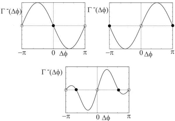
whereΓ⁻(ϕ) = Γ12(ϕ)_{− Γ}12(−ϕ). Equilibrium point ∆ϕe^satisfiesΓ⁻(∆ϕe) = 0. When the derivative ofΓ⁻(ϕ) at ϕ = ∆ϕeis negative, the equilibrium point is stable. In Eq. (2.6), the points∆ϕ = 0 and π are equilibrium points, because the function Γ⁻(ϕ) is periodic and odd. We show three types of the functionsΓ⁻(ϕ) in Fig. 2.2. The solid curve represents the functionΓ⁻(ϕ), the point denotes the stable point, and the circle means the unstable point. The upper left and upper right panels indicate a in-phase and an anti-phase synchronization of the two oscillators, respectively. On the other hand, two oscillators are synchronized with a phase shift in [0, 2π) in case of the lower panel. This type of synchronization is called out-of-phase synchronization.

(32)

∆φ

Γ (∆φ)

∆φ

0 0

0 −π π ^π

π

−π

- _{Γ (∆φ)} ^-

Γ (∆φ) ^-

Figure 2.2: Equilibrium points and their stabilities. The solid curve indicate the functionsΓ⁻(φ) = Γ(φ)−Γ(−φ) and its zero-crossing means the equilibrium point of Eq.(2.6). The point and the circle shows that the equilibrium points are stable and unstable, respectively. Two symmetric connected oscillators are synchronized at in-phase, anti-phase and out-of-phase as shown in the upper-left panel, the upper-right panel and the lower panel, respectively.

2.2 Application in neuroscience

2.2.1 Mathematical model of neuron and synaptic transmission

To apply this theory to neuroscience, we discuss a system given by two neurons, which is synaptically inputted from neuron B to neuron A as shown in Fig. 2.3. Here, we assume that activities of both neurons are represented by the same nonlinear oscillator. Thus, the connected neurons can be considered as a example of coupled phase oscillators. In this section, we explain how to derive the coupling function Γ(ϕ) between the two neurons. The discussion in this section is easily extend toN synaptically connected neurons.

(33)

2.2. APPLICATION IN NEUROSCIENCE 33

dendrite

axon soma

dendrite

AP EPSP

synapse

Neuron A Neuron B

Figure 2.3: Synaptic connection from neuron A to neuron B.

For simplicity, neurons are assumed to be represented by conductance-based models [Koch and Schutter, 1999], which include Hodgkin-Huxley model [Hodgkin and Hux- ley, 1952] and Morris-Lecar model [Morris and Lecar, 1981]. The dynamics of neuron B connected from neuron A is described by the equations for the membrane potentialv and the activities of ionic channelsu⁽¹⁾, . . . , u^(d−1):

c^dv dt ⁼

d−1

∑

i=1

gi(u⁽ⁱ⁾)(v_{− v}i) + iext+ isyn, (2.7) du^(j)

dt ^{= f}

(j)_{(v, u}(1), . . . , u^(d−1)), j = 1, . . . , d_{− 1,} (2.8)

wherec is the membrane capacitance, g_i is the voltage-dependent conductance of thei-th ionic current, and vi is its reversal potential. The current iext represents external inputs besides that from neuron A. The synaptic currentisynfrom neuron A is usually modeled as

isyn =_−gsyn(v_{− v}syn)

Npre

∑

j=0

α(t_{− t}^spike_j ), (2.9)

where gsyn is the maximal synaptic conductance and vsyn is the reversal potential of the synapse. The summation in Eq. (2.9) means the total effect of all the spikes from neuron A,

(34)

wheret^spike_j is the timing of each spike, andNpre is the number of the spikes. The function α(t), which is called alpha function, is defined by

α(t) =







t

τ ^exp^{− t−τ

τ ^{} , t ≥ 0,}

0, t < 0.

(2.10)

In Eqs.(2.7) and (2.8), the interaction between the two neurons is represented by the synaptic currentisyn; i.e. we can assume the form of the interaction in Eq.(2.1) is V1,2 = (isyn, 0, . . . , 0). The dynamics of coupling oscillators defined by Eq.(2.4) are affected from the interaction V_1,2 through the form of the inner product V_1,2· Z(ϕ) in Eq.(2.5). Thus, all components without the voltage componentZ(ϕ) of the PRC Z(ϕ) can be neglected. This is why the voltage componentZ(ϕ) of the PRC gives sufficient information to analyze the synchronization of neurons.

2.2.2 Coupling function between neurons

To compute the coupling functionΓ(ϕ) between the two neurons, we assume that the summation in Eq.(2.9) is approximated as

αT(t) =

−∞

∑

n=0

α(t_{− nT ),} (2.11)

because the activity of neuron A is periodic and its period is T [Vreeswijk et al., 1994]. Using these two formulas

∞

∑

n=0

rⁿ = ¹ 1_{− r}^,

∞

∑

n=0

nrⁿ = ^r

(1_{− r)}²^, |r| < 1, ^(2.12) the periodic functionαT(t) is expressed as

αT(t) = ¹ τ ^exp

{

−^t^{− τ}_τ ^{} t(1}^{− e}

−_{T /τ}

)_{− T e}⁻^{T /τ}

(1_{− e}⁻^{T /τ})² ^. ^(2.13) The coupling function defined by Eq.(2.5) is

(35)

Γ(ϕ) = ¹ 2π

∫ 2π 0

Z(θ)_{−gsyn(v^∗(θ)_{− v}syn)α^∗_T(θ + ϕ)_{} dθ,} (2.14) ,where Z(θ) is the voltage component of the PRC of neuron B, v^∗(θ) = v(θ/ω0), and α^∗_T(θ) = αT(θ/ω0).

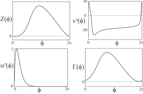
Here, we show the example of the computation of the coupling function Γ(ϕ), when neuron B is represented by Morris-Lecar equations. Using the operational definition in Sec. 1.2, the PRC of neuron B is derived as shown in the upper-left panel of Fig. 2.4. The normalized voltagev^∗(ϕ) and the periodic function α^∗_T(ϕ) are shown in the upper-right and lower-left panels, respectively. By numerically integrating Eq.(2.14), the coupling function is computed as the lower-right panel.

0 2_π

0

φ

Ζ(φ)

-30 0 30

0

_φ

2_π

v

^*

(φ)

0 1

0

_φ

2_π

α (φ)

φ

*

0

_φ

2_π

Γ(φ)

φ

Figure 2.4: The voltage componentZ(φ) of the PRC of Morris-Lecar equations is shown as the curve in the upper-left panel. The curves in the upper-right panel and the lower-left panel are the normalized voltage v^∗(φ) and the function α^∗(φ), respectively. The coupling function Γ(φ) as shown in the lower-right panel is computed using the Eq. (2.14).

By using the function Γ⁻(ϕ) = Γ(ϕ)− Γ(−ϕ), we can analyze the synchronization

(36)

property of the two neurons as discussed in Sec. 2.1. Here, we assume neuron A and neuron B have the same PRCs and are symmetrically connected. When the coupling function is expressed as the lower-right panel in Fig. 2.4, the functionΓ⁻(∆ϕ) is shown in Fig. 2.5. The circle and the point in Fig. 2.5 represent the instability and the stability of equilibrium points of the phase difference∆ϕ = ϕ1 − ϕ2 between the two neurons, respectively. Figure 2.5 shows that the two neurons are synchronized at anti-phase.

0 _π

-_π

Γ (∆φ)

^-

∆φ

Figure 2.5: The functionΓ⁻(∆φ)

2.2.3 Type-I and Type-II phase response curves

Using the functionΓ⁻(ϕ), Hansel et al. [1995], et al. discuss a synchronization property of two symmetrically connected neurons, whose periods and PRCs are the same. By their analysis, the following two types of PRCs are classified:

• in Type I, the value of the PRC Z(ϕ) is positive for all phases ϕ ∈ [0, 2π) as shown in the left panel of Fig. 2.6, whereas

• in Type II, the value of the PRC is negative for a phase as shown in the right panel of Fig. 2.6.

They conclude that the two neurons are not synchronized at in-phase, when the PRCs of the neurons are Type I.

(37)

0 2_π

0

φ

Ζ(φ)

₀

0

_φ

2_π

Ζ(φ)

Figure 2.6: The Type-I and Type-II PRCs.

2.2.4 Usages of phase response curves in neuroscience

Here, we explain why PRCs are used in neuroscience. From the theoretical viewpoint, the dynamical system defined by Eq.(2.4) is easier for analyzing synchronizations than that defined by Eq.(2.1). Many mathematical models of a neuron are proposed to define the vector field f(u) in Eq.(1.2). For example, the leaky integrate-and-fire model [Koch and Schutter, 1999], Hodgkin-Huxley model [Hodgkin and Huxley, 1952], and Morris- Lecar equations [Morris and Lecar, 1981] are widely used in computational neuroscience. However, mathematical analysis based on the models is difficult, because the vector field f(u) is complicated (except for the leaky integrate-and-fire model). On the other hand, the dynamical system defined by Eq.(2.4) is usually simpler than the original dynamics. Actually, a lot of mathematical analysis is done based on Eq.(2.4) [Kuramoto, 1984, Tsubo et al., 2007a].

Moreover, computer simulations based on Eq.(2.4) are easier than that based on Eq.(2.1) [Gal´an et al., 2006], because the number of the dimension of the state (ϕ₁, . . . , ϕ_N) in Eq.(2.4) is1/d times of that of the state (u1, . . . , uN) in Eq.(2.1).

(38)

(39)

Chapter 3

Estimation of phase response curves

3.1 Measurement of phase response curves

Measurements of PRCs are conventionally based on the operational definition of Sec. ??. However, in experiments, inter-spike intervals fluctuate stochastically [Mainen and Se- jnowski, 1995] as shown in the upper-left panel of Fig. 3.1. The period T in Eq. (1.1) is conventionally replaced by the average ˆT of the inter-spike intervals. The data point (xi, yi) from the measurement is expressed as

x_i = 2π^tⁱ

Tˆ^, ^yⁱ ^{= 2π}

Tˆ_{− T}_i^′

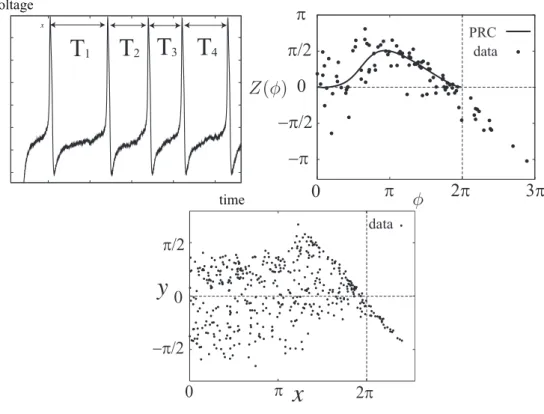
Tˆ i = 1, . . . , n. (3.1) The data points _{(x_i, yi)} in the upper-right panel are generated with noisy Morris-Lecar equations explained in Appendix. B. The data in the lower panel are experimentally measured, which we discuss in Sec. 7.2.1. Note that the data point whose valuexi _{≥ 2π exist}

in the example. This is one of key observations in this chapter. 39

(40)

40 CHAPTER 3. ESTIMATION OF PHASE RESPONSE CURVES

voltage

time

T

¹

T

2

T

³

T

⁴

x PRC

data

x

y

Figure 3.1: The left panel shows fluctuation of the periods. Theith inter-spike interval is denoted byT_ifori = 1, 2, 3, 4. Examples of the data is in the middle and right panels.

3.2 Previous studies

Fourier regression

In most existing studies, the PRC is estimated from the data_{(x_i, yi)} in Sec. 3.1 based on the normal regression model

yi = Z(xi) + εi, εi _{∼ N (0, σ}²), , i = 1, . . . , n (3.2) where the error in the response variable is represented byεi, and the variance of the error is σ². In the regression model, the valuexiis assumed to be less than2π, because the domain of the PRC is [0, 2π). R. F. Gal´an and his collaborators [Gal´an et al., 2005] proposed a

(41)

3.2. PREVIOUS STUDIES 41

representation of the PRCZ(ϕ) as the finite Fourier series

Z(ϕ) = ^a⁰ 2 ⁺

3

∑

k=1

akcos(kϕ) + bksin(kϕ). (3.3)

We call this method “Fourier regression” in this thesis. An example of the estimate is shown in Fig. 3.2, where the data points whose valuex_i ≥ 2π are removed.

Fourier regression data

Figure 3.2: An example of the estimate obtained through Fourier regression

Spline regression

For estimating PRCs, Ke. Ota and his collaborators proposed a Bayesian method [Aonishi and Ota, 2006, Ota et al., 2009b] with a smoothing prior, where the representation of the PRC is based on high order Fourier series. Their method can deal with data generated with various types of experiments, where arbitrary input is injected to a neuron. When the injection is a pulse, their method essentially corresponds to Bayesian regression based on the normal regression model.

In this thesis, we introduce another Bayesian regression with a smoothing prior (see Secs. 5.3 and 5.3), the framework of which is proposed by Tanabe and Tanaka [1983]. It is convenient for our method proposed in part II. This Bayesian regression is also based on the normal regression model. Hereafter, we call the Bayesian regression “spline regression”. The estimate through the spline regression is shown in Fig. 3.3.

(42)

In this thesis, “conventional regression” means the method based on the normal regression model Eq.(3.2), where no errors exist in explanatory variable. The Fourier regression and the spline regression are the examples of the conventional regression.

spline regression data

Figure 3.3: An example of the estimate obtained through spline regression

Other methods for different types of data

Recently, some methods are proposed for estimating PRCs using different types of data discussed in Sec. 3.1.

Phoka et al. [2010] proposes that supplemental data are added to the data explained in Sec. 3.1 using inter-spike intervals before and after the input of a neuron. The drawback of this method is that the estimated PRCs can not be a periodic function.

Ermentrout et al. [2007] and Ota et al. [2009a] propose that white and correlated noises are injected to a neuron, respectively. These experiments can be alternatives to the conventional experiments supposed in this thesis, although there are applications that would be difficult to treat with this approach, e.g., circadian rhythm.

Oprisan et al. [2003] estimates PRCs using the limit cycle reconstructed from membrane potential of a neuron. The PRCs estimated by this method correspond to PRCs where the strength of inputs are large in the operational definition of Sec. ??; however, the strength should be small because of the definition from dynamical viewpoints in this thesis.

(43)

3.3. MEASUREMENT ERROR MODEL 43

3.3 Measurement error model

The existence of the data point whose value x_i ≥ 2π implies errors in the explanatory variable. In my master thesis [Nakae, 2008], we discuss a measurement error model, where both errors in the explanatory and response variables are considered [Amari and Kawanabe, 1997, Cheng and Ness, 1999, Berry et al., 2002, Fuller, 2006, Caroll et al., 2006]. The measurement error model is expressed as

xi = ϕi+ (εx)i, (εx)i ∼ N (0, (σ²x⁾ⁱ^), ^(3.4)

y_i = Z(ϕ_i) + (ε_y)_i, (ε_y)_i _{∼ N (0, σ}_y²), , i = 1, . . . , n, (3.5) where we assume that the variance (σ_x²)i is proportional toxi. The representation of the PRCZ(ϕ) in this model is that of the spline regression. In this model, the error (εx)i^{in the}

explanatory variable and the error(ε_x)_iin the response variable are independent each other; the errors are not correlated. Unfortunately, we did not achieve a significant improvement over conventional regression in terms of accuracy.

3.4 Characteristics of errors in the data

In this section, we discuss two characteristics of errors in the data_{(x_i, yi)} as follows: 1. The data point(xi, yi) whose value xi ≥ 2π exist.

2. All data points are in the regionK ={(x, y) ∈ R²|x ≥ 0, x + y ≤ 2π}; as shown in the right panel of Fig. 3.4.

Characteristic 1 is caused by a perturbation inputted at the timingti > ˆT as shown in the left panel of Fig. 3.4. Conventional regression can not deal with such data, because the domain of PRC is[0, 2π).

Characteristic 2 is a consequence of the two inequalities for alli = 1, . . . , n x_i = 2π^tⁱ

Tˆ ^{≥ 0,} ^(3.6)

(44)

xi+ yi = 2π^tⁱ Tˆ ^{+ 2π}

Tˆ_{− T}_i^′

Tˆ ^{= 2π}⁻ 2π

Tˆ ^(T

′

i − ti)_{≤ 2π,} (3.7) which are derived by the definition of the data point Eq.(3.1) and the trivial two inequalities ti _{≥ 0 and t}i _{≤ T}_i^′^.

The measurement error model Eqs. (3.4) and (3.5) is not sufficient; it generates the data points outsideK, especially above the line x + y = 2π. This is because the error (εx)i^and

the error(εy)i are independent each other.

voltage

current

i i

x

y

K

Figure 3.4: Two characteristics of the data.

3.5 Our Approach

The discussion in the previous section implies that the errors in the explanatory and response variables are not independent each other; the errors are correlated. Our motivation in this thesis is developing a statistical method dealing with the correlation.

In part II, we propose a statistical model, which represents a correlation between the explanatory and response variables. Based on the model, we provide a Bayesian method for estimating the PRCs using replica exchange Monte Carlo methods. In numerical experiments, we show that estimates obtained through the proposed method are more accurate than those obtained through conventional regressions.

Unfortunately, massive parallel computing environments are necessary for actual use

(45)

3.5. OUR APPROACH 45

of the proposed method. Without parallel computing, computation time of the proposed method is about 3 days for a sample size n = 100. On the other hand, computation time with parallel computing is reduced to approximately2 hours for the same sample size. Our motivation of part III is developing a more efficient method based on the model proposed in part II.

In part III, the correlation is effectively removed using a transformation that mixes the explanatory and response variables. We show that the method through the transformation gives more accurate estimator than conventional regressions and the computation time is considerably less than that of the method in part II.

(46)

(47)

Chapter 4

Bayesian estimation and Markov chain

Monte Carlo methods

4.1 Bayesian framework

In this section, we briefly explain a Bayesian framework used in this thesis. Suppose that observations y =_{yi|i = 1, . . . , n} are independent and identically distributed; the distribution of the observations is depend onM -dimensional variables γ = (γ⁽¹⁾, . . . , γ^{(M )})_{∈ Γ} and M^′-dimensional variables θ ∈ Θ. The density function of the observation is represented by pγ(y|θ). Here, the variables θ called “parameters” are assumed to be random variables, while the variables γ called “hyperparameters” are assumed to be not random variables. The prior density of θ is denoted by pγ(θ). The joint density of y and θ is defined as

pγ(y, θ) = pγ(y_|θ)pγ(θ). (4.1) We estimate the hyperparameters γ and the parameter θ from the observations y. The hyperparameters γ is estimated by an empirical Bayesian method [Good, 1965, Akaike, 1980, Titterington, 1985, MacKay, 1992] that maximizes the marginal likelihood

lγ(y) =

∫

θ∈Θ

pγ(y, θ)dθ (4.2)

over Γ. Once the estimate ˆγ are obtained, the posterior densitypγˆ(θ|y) is derived by the 47

(48)

48CHAPTER 4. BAYESIAN ESTIMATION AND MARKOV CHAIN MONTE CARLO METHODS

Bayes’ theorem

pγˆ(θ_{|y) =} ^p^γ^ˆ^(y^|θ)p^γ^ˆ^(θ)

lγˆ(y) ^. ^(4.3)

In the following sections, the parameter θ is estimated by the expectation of θ over the posterior distribution

Epos[θ] =

∫

θ∈Θ

θpγˆ(θ_|y)dθ. (4.4)

The estimate is denoted by ˆθ.

4.2 Markov chain Monte Carlo methods

4.2.1 Metropolis-Hastings method

The estimatesγ and ˆˆ θ are automatically derived using the framework in the previous section. It is, however, difficult to give analytical representations of the marginal likelihood in Eq. (4.2) and the posterior expectation in Eq. (4.4), when the likelihood pγ(y_{|θ) and} the priorpγ(θ) are complicated. In this section, we explain a Metropolis-Hastings method [Hastings, 1970], which is one of Markov chain Monte Carlo (MCMC) methods, for ap- proximating the integral in Eq. (4.4). The Metropolis-Hastings (MH) method is extended to a replica exchange Monte Carlo (REM) method [Geyer, 1991, Hukushima and Nemoto, 1996, Iba, 2001] in the next section. In Chap. 6, we will explain how to maximize the marginal likelihood in Eq. (4.2) based on the MCMC methods.

In the MCMC methods, the posterior expectation of θ is approximated by the average of samples from the MCMC methods

Epos[θ]_≈ ¹ NMC

NMC

∑

j=1

θ^j, (4.5)

where NMC is the number of the samples, and θ^j is jth sample. These samples are generated by the following procedure called Metropolis-Hastings methods. Here, we define a conditional distribution as a proposal distribution, whose density is represented byq(θ^′_|θ).

• Choose θ¹in the regionΘ. Forj = 1, . . . , NMC−1

(49)

4.2. MARKOV CHAIN MONTE CARLO METHODS 49

• Generate a candidate θ^cand ∼ q(θ^′|θj)

• Take

θj+1 =







θ^cand with the probabilityr,

θ_j otherwise,

(4.6)

where

r = min^{{ p}^γ^{(y, θ}

cand_)q(θcand

|θ^j⁾ pγ(y, θ^j)q(θ^j_|θ^cand) ^{, 1}

}

. (4.7)

Note that θ^j+1 = θ^j, when the candidate θ^candis out of the regionΘ.

This procedure defines a Markov chain with the stationary density pγ(θ|y) on some convergence properties [Robert and Casella, 2004]. By simulating the Markov chain, we can draw samples of θ according to the posterior density. Details of the general theory of MCMC can be found in books by [Robert and Casella, 2004, Gilks et al., 1995, MacKay, 2003, Gelman et al., 2003].

4.2.2 Replica exchange Monte Carlo method

The procedure explained in the previous section is a standard example of MCMC methods used in Bayesian statistics. It works if the number of iterations is sufficiently large. How- ever, the number of iterations necessary to obtain stable results using such an algorithm can be very large in a complicated problem, which is known as “slow mixing” or “slow relaxation”. We will encounter the problem in part II of this thesis, where we can barely get stable results using a MH method in a range of hyperparameters.

To deal with this difficulty, we introduce the replica exchange Monte Carlo (REM) method, which is also known as parallel tempering or Metropolis coupled MCMC [Geyer, 1991, Hukushima and Nemoto, 1996, Iba, 2001].

REM is designed to increase the efficiency of MCMC method by connecting a fast mixing “easy” region to the slow mixing “difficult” region. The REM shares this idea with the simulated annealing algorithm for optimization, but there is an important difference. While simulated annealing is designed for obtaining an optimal solution and does not necessarily reproduce correct averages of statistics with a given distribution, the REM is designed for correct sampling and calculation of averages.

本文 総合研究大学院大学学術情報リポジトリ 甲1420 本文

Statistical Estimation of Phase Response Curves

Ken Nakae

DOCTOR OF PHILOSOPHY

Department of Statistical Science

School of Multidisciplinary Science

The Graduate University for Advanced Studies

2010 (School Year)

Abstract

Acknowledgment

Overview of this thesis

Contents

Part I

Background and motivation

Chapter 1

Introduction

1.1 Synchronization

observation

color

shape

This is a brown disc. spikes

synchronization

recognition

1.2 Phase response curves and coupled phase oscillators

Step 1 Step 2

Step 3

C S

u (t)

φ(t)

phase reduction

1.3 Phase response curves in neuroscience

φ

Ζ (φ)

φ

Ζ (φ)

Ζ (φ)

φ

Ζ (φ)

φ

φ

Ζ(φ)

φ

Ζ(φ)

1.4 Motivation of this thesis

2π

0

response

0 phase x 2π

y

K

Chapter 2

Theory of synchronization

2.1 Coupled phase oscillators

Γ(φ − φ )

φ (t)

φ (t)

Γ(φ − φ )

∆φ

Γ (∆φ)

∆φ

∆φ

0 0

0

−π π π

π

−π

−π

- Γ (∆φ) -

Γ (∆φ) -

2.2 Application in neuroscience

Neuron A Neuron B

φ

Ζ(φ)

φ

v

(φ)

φ

α (φ)

φ

φ

本文総合研究大学院大学学術情報リポジトリ甲1420 本文

This is a brown disc. _spikes

Step 1 ^{Step 2}

C _S

u _(t)

_φ

0 _phase _x ^2π

^{φ (t)}

−π π ^π

- _{Γ (∆φ)} ^-

Γ (∆φ) ^-

_φ

_φ

_φ

_φ