本文 Thesis 総合研究大学院大学学術情報リポジトリ A1715本文

The Graduate University for Advanced Studies

Shonan Village, Hayama, Kanagawa 240-0193 Japan

Author

PHAN Hong Khiem

Full one-loop electroweak radiative

corrections at Future Colliders

Supervisor

Prof. Yoshimasa KURIHARA Referees

Prof. Shoji HASHIMOTO (Head Examiner) Prof. Junpei FUJIMOTO (Examiner)

Prof. Kyoshi KATO (Examiner)

Prof. Mihoko NOJIRI (Examiner) Prof. Shigeru ODAKA (Examiner) Prof. Keisuke FUJII (Examiner)

KEK-18th December 2014

Table of Contents i

Abstract xiii

Acknowledgements xv

Introduction xix

1 The Standard Theory and beyond 1

1.1 The Standard Theory . . . 1

1.1.1 The classical Lagrangian . . . 2

1.1.2 Quantization: gauge-fixing and ghost Lagrangian . . . 6

1.2 Beyond the Standard Theory . . . 7

2 GRACE-Loop 11 2.1 Motivation of the automatic calculation . . . 11

2.2 Introduction to GRACE-Loop . . . 15 i

ii

2.3 One-loop renormalisation . . . 19

2.3.1 Renormalisation scheme . . . 25

2.4 Tensor one-loop reduction . . . 27

2.4.1 Scalar one-loop N ≤ 4 point integrals . . . ²⁸

2.4.2 Tensor one-loop 2-point reduction . . . 29

2.4.3 Tensor one-loop 3-, and 4-points reduction . . . 30

2.4.4 Tensor one-loop 5-point reduction . . . 33

2.5 Tensor one-loop 5-point reduction in LoopTools . . . 35

2.6 Test on the calculation with GRACE-Loop . . . 37

2.6.1 Ultraviolet finiteness . . . 37

2.6.2 Infrared finiteness . . . 37

2.6.3 Gauge-parameters independence checks . . . 39

2.6.4 kc stability . . . 39

3 Full one-loop electroweak radiative corrections to the W -pair pro- duction in association with a jet at the LHC 41 3.1 The Large Hadron Collider . . . 41

3.2 Motivation of the calculation . . . 44

3.3 Calculation of pp → W^+W−+ 1 jet at the LHC . . . 47

3.3.1 Setup of the calculation . . . 47

3.3.2 Numerical checks . . . 51

3.3.3 Physical results . . . 53

4 Full O(α) electroweak radiative corrections to e^+e− → e^{+e−γ at the} ILC 61 4.1 Luminosity measurement at ILC . . . 61

4.2 The process e⁺e⁻_{→ e}⁺e⁻γ at the ILC . . . 64

4.2.1 The calculation . . . 64

4.2.2 Numerical check . . . 66

4.2.3 The physical results . . . 67

5 Full O(α) electroweak radiative corrections to the processes e^+e−→ t¯t and e⁺e⁻ → t¯tγ at the ILC ⁸¹ 5.1 Top quark physics at the ILC . . . 82

5.2 The process e⁺e⁻→ t¯t at the ILC . . . ⁸⁷

5.3 The process e⁺e⁻→ t¯tγ at the ILC . . . ⁹³

6 Conclusions 103 A The counterterm 105 B The input parameters 109 C The numerical checks 111 C.1 The process pp → W^−W++ 1 jet . . . 111

iv

C.2 The process e⁻e⁺_{→ e}⁻e⁺γ . . . 113 C.3 The process e⁻e⁺→ t¯t . . . 114 C.4 The process e⁻e⁺→ t¯tγ . . . 116

D The phase space integration 119

D.1 Two-body phase space integral . . . 119 D.2 The n-body phase space integral . . . 120

E The F function 125

Bibliography 127

2.1 The GRACE-Loop flow chart. . . 17 2.2 General structure of the one-loop N-point integral. The figure is taken

from the paper [21]. . . 28 2.3 Feynman diagrams in the process e⁺e⁻ _{→ e}⁺e⁻γ generated by the

GRACE-Loop program. . . 38

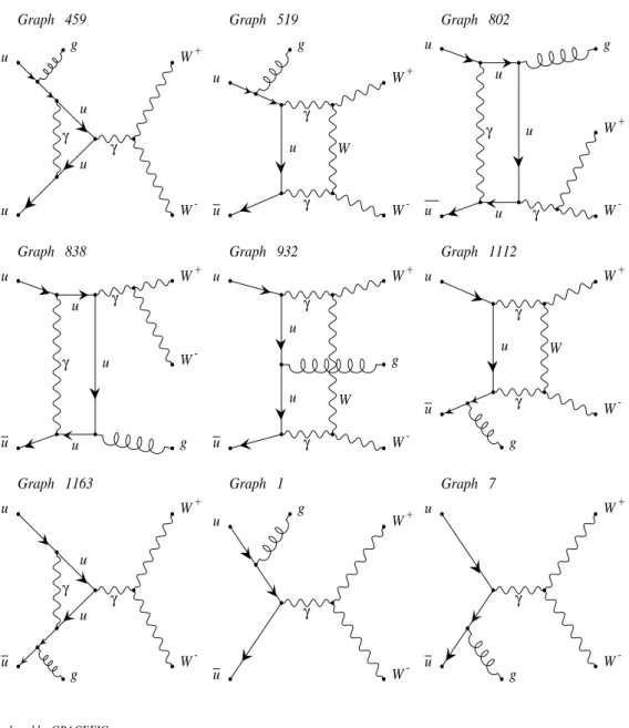
3.1 ATLAS and CMS experiments reported evidence for new boson. . . . 45 3.2 Selected Feynman diagrams are generated by the GRACE-Loop program. 50 3.3 Distributions of cross-section (left) and full electroweak corrections

(right) are presented as a function of PT,jet. . . 57 3.4 Distribution of cross-section is presented as a function of the pseudo-

rapidity of the jet. . . 58

4.1 Selected Feynman diagrams are generated by the GRACE-Loop program. 65 4.2 In this figure, the cross-section (upper) and full electroweak corrections

(right) are presented as a function of the center-of-mass energy. . . . 69 4.3 The differential cross-sections as a function of the photon energy at

√s = 250 GeV (left) and^√s = 1 TeV (right). The bottom figures are the K_EW factor which is a function of photon energy. . . 71

v

vi

4.4 The differential cross-sections as a function of the positron’s energy. At

√s = 250 GeV (left) and at^√s = 1 TeV (right). The bottom figures present for the KEW factor. . . 72 4.5 The differential cross sections are a function of the invariant mass of

the e⁻, e⁺ pair. The left figure is at^√s = 250 GeV and the right figure is at ^√s = 1 TeV. . . 74 4.6 The differential cross-sections as a function of the invariant mass of the

e⁻, photon. The left figure is at ^√s = 250 GeV and the right figure at

√s = 1 TeV. . . 75

4.7 The angular distributions of photon are shown at ^√s = 250 GeV and

√s = 1 TeV. . . 76

4.8 The angular distributions of positron in final states are shown at^√s = 250 GeV and ^√s = 1 TeV. . . 77 4.9 The angular distributions of opening angle between photon and elec-

tron in the final states. The left figure is at ^√s = 250 GeV and the right figure is at ^√s = 1 TeV. . . 78

5.1 The currently stage of the accuracy from QCD calculation is presented. The figure is taken in Ref [114]. . . 83 5.2 A comparison of precision for CP conserving form factors of top quark

couplings to γ and the Z boson at LHC and ILC. The figure is taken in Ref [118]. . . 85 5.3 The total cross-section and the full electroweak corrections as a func-

tion of the center-of-mass energy ^√s. . . 90 5.4 The angular distributions of the top quark at ^√s = 500 GeV and

√s = 1 TeV. . . 91

5.5 The top quark forward-backward asymmetry and its electroweak cor- rection as a function of the center-of-mass energy. . . 92 5.6 Selected Feynman diagrams generated by the GRACE-Loop program. 94 5.7 The total cross-section and the full electroweak corrections are pre-

sented as a function of the center-of-mass energy^√s. . . 96 5.8 The distribution of the cross section as a function of photon energy at

√s = 500 GeV (left figure) and at^√s = 1 TeV (right figure). . . 97

5.9 The angular distributions of photon at ^√s = 500 GeV and at 1 TeV. 99 5.10 The angular distributions of top at^√s = 500 GeV and at 1 TeV. . . 100 5.11 The distributions of the cross section as a function of the invariant

mass of the top quark and photon (mγt) at^√s = 500 GeV and ^√s = 1 TeV. . . 101 5.12 The top quark forward-backward asymmetry and its electroweak cor-

rections as a function of the center-of-mass energy. . . 102

A.1 One-loop vertex diagrams which contributed to the g → u¯u . . . 106

D.1 The diagrammatic representation of splitting phase space of n particle. 122 D.2 In the CMS (1 + 2). . . 123

List of Tables

1.1 The Standard Theory of elementary particles, with the three genera- tions of fermions, gauge bosons in the fourth column, and the Higgs boson in the fifth. . . 2

2.1 The number of Feynman diagrams in the covariant gauge. NLoop diagrams

includes one-loop virtual diagrams and counterterm diagrams. . . 13 2.2 The prediction for M_W as a function of M_H at M_Z = 91.1876 GeV and

mt= 173.5 GeV. . . 26 2.3 Test of the reduction of the one-loop five-point functions in GRACE-

Loop in comparison with the method in Ref [16]. . . 37

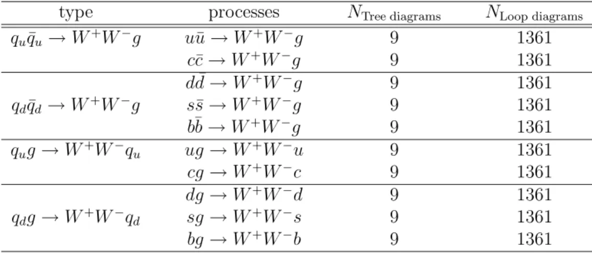
3.1 LHC beam parameters relevant for the peak luminosity [69] . . . 43 3.2 The partonic processes contribute to the process pp → W^{+W−+ 1 jet}

at the LHC. . . 49 3.3 Number of Feynman diagrams of the partonic processes are generated

by GRACE-Loop. . . 49 3.4 Result of the Ward-identities tests. . . 51 3.5 Result of the Ward-identities tests in the partonic cross section. . . . 52

ix

3.6 Cross-check of the result in this calculation with the paper [77] by varying the p^cut_T,W of the W boson at 14 TeV of the LHC. . . 54

3.7 Cross-check of the result in this calculation with the paper [77] by changing the invariant mass cut of the W-pair, (M_W^cut−_W+) at 14 TeV of the LHC. . . 55

3.8 The cross section and electroweak corrections are shown for the LHC 14 TeV. . . 57

4.1 The problem with large numerical cancellation. . . 66

4.2 The result must be independent of the choice of gauge for photon. . . 66

5.1 Comparison of the total cross section e⁺e⁻→ t¯tbetween this work and [128]. The corrections refer to the full one-loop electroweak corrections including hard photon radiation. . . 88

C.1 Test of the CU V independence of the amplitude. In this table, we take the non-linear gauge parameters to be 0, λ = 10⁻¹⁷GeV and we use 1 TeV for the center-of-mass energy. . . 111

C.2 Gauge invariance of the amplitude. In this table, we set CU V = 0, the photon mass is 10⁻¹⁷GeV and a 1 TeV center-of-mass energy. . . 112

C.3 Test of the IR finiteness of the amplitude. In this table we take the non-linear gauge parameters to be 0, CU V = 0 and the center-of-mass energy is 1 TeV. . . 112

xi

C.4 Test of the k_c-stability of the result. We choose the photon mass to be 10⁻¹⁷ GeV and the center-of-mass energy is 200 GeV. The second column presents the hard photon cross section and the third column presents the soft photon cross section. The final column is the sum of both. The statistical error of integration step is below 0.1% for this test. . . 112 C.5 Test of the CU V independence of the amplitude. In this table, we take

the non-linear gauge parameters to be 0, λ = 10⁻¹⁷GeV and we use 1 TeV for the center-of-mass energy. . . 113 C.6 Gauge invariance of the amplitude. In this table, we set CU V = 0, the

photon mass is 10⁻¹⁷GeV and a 1 TeV center-of-mass energy. . . 113 C.7 Test of the IR finiteness of the amplitude. In this table we take the

non-linear gauge parameters to be 0, CU V = 0 and the center-of-mass energy is 1 TeV. . . 113 C.8 Test of the kc-stability of the result. We choose the photon mass to be

10⁻¹⁷ GeV and the center-of-mass energy is 1 TeV. The second column presents the hard photon cross-section and the third column presents the soft photon cross-section. The final column is the sum of both. The statistical error of integration step is below 0.1% for this test. . . 114 C.9 Test of CU V independence of the amplitude. In this table, we take the

non-linear gauge parameters to be 0, λ = 10⁻¹⁷GeV, kc = 0.001 GeV and we use 1 TeV for the center-of-mass energy. . . 114 C.10 Test of the IR finiteness of the amplitude. In this table we take the

non-linear gauge parameters to be 0, CU V = 0, kc = 0.001 GeV and the center-of-mass energy is 1 TeV. . . 115 C.11 Gauge invariance of the amplitude. In this table, we set CU V = 0, the

photon mass is 10⁻¹⁷GeV and a 1 TeV center-of-mass energy. . . 115

C.12 Test of the k_c-stability of the result. We choose the photon mass to be 10⁻¹⁷ GeV and the center-of-mass energy is 1 TeV. The second column presents the hard photon cross-section and the third column presents the soft photon cross-section. The final column is the sum of both. The statistical error of integration step is below 0.1% for this test. . . 115 C.13 Test of CU V independence of the amplitude. In this table, we take the

non-linear gauge parameters to be 0, λ = 10⁻¹⁷GeV and we use 1 TeV for the center-of-mass energy. . . 116 C.14 Test of the IR finiteness of the amplitude. In this table we take the

non-linear gauge parameters to be 0, CU V = 0 and the center-of-mass energy is 1 TeV. . . 116 C.15 Gauge invariance of the amplitude. In this table, we set C_{U V} = 0, the

photon mass is 10⁻¹⁷GeV and a 1 TeV center-of-mass energy. . . 116 C.16 Test of the kc-stability of the result. We choose the photon mass to be

10⁻¹⁷GeV and the center-of-mass energy is 1 TeV. The second column presents the hard photon cross-section and the third column presents the soft photon cross-section. The final column is the sum of both. The statistical error of integration step is below 0.1% for this test. . . 117

Abstract

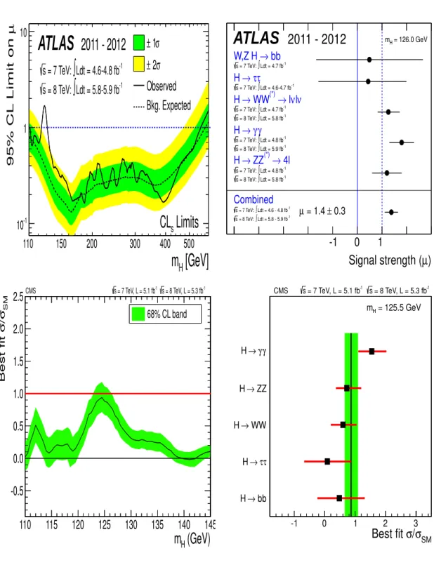
In July 2012, ATLAS and CMS experiments at the Large Hadron Collider (LHC) announced the evidence for a new boson whose properties were consistent with the SM Higgs boson [1, 2, 3, 4, 5, 6]. The mass of the new boson was reported by two experiments as

ˆ ATLAS: 126.0 ± 0.4(stat.)±0.4(sys.) GeV;

ˆ CMS: 125.3 ± 0.4(stat.)±0.4(sys.) GeV.

Once the discovery of the Higgs boson is confirmed, it will open a new phase for studying particle physics. The expected program of future colliders, e.g. the high luminosity version of LHC, the International Linear Collider (ILC), not only makes precise measurements on the properties of the Higgs particle, top quarks and vector bosons interactions, but also search for physics Beyond the Standard Theory. The measurements will be performed at high precision. In order to match future precision data, the theoretical calculations to the experimental measurement such as cross section and decay width, with including higher order radiative corrections are mandatory. The calculations are great motivation and effort by many groups. Such calculations are one of the main targets of this thesis. In particular, the aim of thesis is twofold:

1. The first aspect of the thesis is to study how to calculate the experimental quantities in the framework of Quantum Field Theory. This part is mainly

xiii

focused to upgrade the GRACE-Loop program which is a generic automatic computer program for calculating High Energy Physics processes at one-loop electroweak corrections.

2. The second aspect of the thesis is to apply the above framework to compute the full O(α) electroweak radiative corrections to some of the most important processes at future colliders. These processes are

ˆ _{pp → W}

−_W+ _{and pp → W}−_W++ 1 jet at the LHC;

ˆ _e

−_e+ _{→ e}−_e+γ at the ILC;

ˆ _e

−_e+ → t¯t and e^−e+→ t¯tγ at the ILC.

We observe that electroweak radiative corrections to W -pair production and W -pair production in association with a jet at the LHC are of sizeable impact (order 10%) in the high-energy region where the new-physics signatures are expected. The cor- rections must be included to interpret the new physics signals at the future LHC experiments.

For the processes at the ILC, the electroweak radiative corrections also form sig- nificant contributions (order 10%). Such corrections are very important contributions and they must be taken into consideration in the future.

Acknowledgements

First of all, I would like to express my deep gratitude to my friendly supervisor, Prof. Yoshimasa KURIHARA, for his inspirational and patient advice, enthusiasm suggestions and constant encouragement during my PhD time. I have learned a great methods from my supervisor perspective on research, the scientific approaches he analyses the Physical problems in a simple and pedagogical way. Moreover, I would like to thank my supervisor so much for his constant support me to attend many interesting conferences and internship program at NIKHEF.

I am deeply indebted to MINAMI-TATEYA GROUP: Prof. Junpei FUJIMOTO, Prof. Toshiaki KANEKO, Prof. Fukuko YUASA, Prof. Kyoshi KATO, Prof. Yoshim- itsu SHIMIZU, Prof. Tadashi ISHIKAWA for their help and enthusiasm suggestions and constant encouragement. I would like to thank Prof. Shigeru ODAKA, Prof. Ken SASAKI and Prof. Tadashi KON, Prof. Masaaki KURODA and Prof. Masato JIMBO, Prof. Y. YASUI for their fruitful discussions. I would like to send my deeply thank to Prof. K. TOBIMATSU, Prof. N. NAKAZAWA and Prof. M. IGARASHI for useful discussions.

I would like to express my deep appreciate to Prof. J.A.M VERMASEREN for giving me a great chance to visit NIKHEF and for his advice during my time in NIKHEF. Thank to Prof. VERMASEREN so much for his effort to read the paper manuscripts and his encouragement.

I am indebted to Dr. DO Hoang Son, my advisor in master program at the

xv

University of Science HoChiMinh City for his advice and enthusiasm suggestions. He has encouraged me so much to attach the difficult problem in Physics and to mature my research method.

Dr. Takahiro UEDA is a good friend, he is very good at computer program, specially he is a master in using and developing FORM. I am deeply indebted to Dr. Takahiro UEDA for his guidance and fruitful discussions about FORM as well as Physics.

I am indebted to Prof. Patrick AURENCHE, Prof. Pietro SLAVICH for support- ing me to have great internship program at LPTHE. I had a great chance and fruitful discussions to Prof. Pietro SLAVICH about the Physics Beyond the Standard Model. My deeply thank directly to Profs. TRAN Thanh Van and NGUYEN Anh Ky for their support and give me many chance to attend Vietnam School of Physics (VSOP). I am grateful to Rencontres du Vietnam sponsored by Odon VALLET. My PhD’s fellowship is supported by Japanese Government Scholarship (MEXT).

I am grateful to Profs. HOANG Dzung, NGUYEN Nhat Khanh, PHAN Quoc Khanh, Dr. NGUYEN Huu Nha at The University of Science HoChiMinh City for their teaching and their encouragement.

My deep appreciate to Prof. KANEMURA and Dr. YOKOYA for giving a chance to visit the University of Toyama and for their fruitful discussions.

I would like to express my deep appreciate to Prof. Mihoko NOJIRI, Prof. Shoji HASHIMOTO, Prof. Keisuke FUJII for give me many comments and suggestions and for their effort to read the manuscripts.

For interesting discussions I would like to thank Prof. Emi KOU, Ms. Nhi M. U. QUACH, Dr. KAWAMURA, Mr. Rottier OTTO, Dr. WATANABE and Dr. LE Duc Ninh, Dr. LE Tho Hue for many fruitful discussions.

I want to send my deeply thank to my colleagues at Thu Dau Mot University,

xvii

Binh Duong, Vietnam: Dr. NGUYEN Van Hiep, Mr. TRAN Quang Thai, Dr. VO Van On for their support.

Life would not have been as colorful without the many good friends I have. I would like to express my deep thank to Mr. LE Van Hung, Mr. NGUYEN Tan Loc, Mr. NGUYEN Truong Co and Mr. PHAN Toai Tuyn. They are always with me to share happiness and disappointment.

Last but not least, I want to thank my warm family for their encouragement. To my wife, NGUYEN Vuong Ngoc Thy and specially for her present of love, our lovely son, PHAN Hoang Khiem for their invaluable love.

It is human nature try to answer the fundamental question. What are the building blocks of matter? An earlier answer to the question was proposed by Thales about 2600 years ago. His concept was that the matter could be reduced to water. One century later, Anaximenes of Miletus thought that the world was made of four ele- ments, such as earth, water, fire and air. Both Thales and Anaximenes’s concepts of the fundamental structure of matter are very simple and economical in the number of building blocks.

In 1869 Mendeleev published the periodic table of elements. The table listed of the elements according to the basis of their atomic weights and recurring columns possessing the same chemical properties. In the Mendeleev’s concept the matter was constructed by these elements. At the same time, many new chemical elements were discovered and arranged them into the table. From the theorist’s point of view one may doubt that ”Are there too many fundamental elements” by looking at the hundred of elements in the table. Are there substructures for these particles?

In 1898 Joseph Thomson discovered that the cathode rays are electron beams. The discovery was a big challenge for the elements in the Mendeleev’s periodic table as units of the Universe. This discovery also opened a new era, i.e the subatomic era. In 1911 Rutherford analyzed the so-called ”plum pudding model” of the atom by J. J. Thomson. He found that this model was incorrect. The model of atom was reformed by Rutherford. In Rutherford’s concept the atom contains highly concentrated charge

xix

xx

and mass in a very small volume at its center which later was named the ”nuclei” of the atom. By 1919, the proton was discovered by Rutherford via¹⁴_{N + α →} ¹⁷O + p. Later, in 1932 James Chadwick found the neutron. The discoveries modified the nice picture of fundamental elements drawn by Mendeleev.

In 1910, Charles Wilson invented the cloud chamber containing a supersaturated vapor of water or alcohol. The cloud chamber allowed us to capture the track of charged particles. Many hadrons thereof like baryons and mesons were discovered one by one in a very short period. In 1964 the quark model was formed by Murray Gell-Mann, Kazuhiko Nishijima and George Zweig. In this model, the hadrons are constructed by the fundamental elements which are called quarks. In 1968, a deep inelastic scattering experiment at the Stanford Linear Accelerator Center (SLAC) showed that the proton contains quarks. The picture of the fundamental elements was refreshed and the gold era of particle physics started.

All these particles discovered through the last century make up the most complete theory, the Standard Theory (SM), which was proposed by Steven Weinberg, Sheldon Glashow and Abdus Salam [7] in 1967. After discovering tau lepton (at SLAC) and bottom, top quarks (at Fermilab), the fundamental building blocks of the SM consist of three charged leptons, three corresponding neutrinos and six quarks in the fermion sectors. These fermions interact via gauge boson exchange: Specially the photon for electromagnetic interaction, the weak gauge bosons Z and W^± for weak interaction, and eight gluons for the strong interaction. In the theory the masses of the bosons are generated through nowadays known as the Higgs-Brout-Englert-Guralnik-Hagen- Kibble mechanism [8, 9]. While the masses of fermions are explained by their strength of interaction with the scalar Higgs boson. Present-day the main goals of particle physics studies are to test the SM and probe the new physics.

The LEP collider [10] was built by European Organization for Nuclear Research (CERN). It is an electron-positron collider with a tunnel of 26.7 kilometer circum- ference at 50–175 meter underground, crossing the Switzerland–France border. The

LEP operated to provide electron-positron collisions from Z peak energies between 89 and 93 GeV up to the highest energies above the W-pair threshold between 161 and 209 GeV. One of the important goals of LEP experimental program was the measurement of the properties of W and Z bosons, such as their masses, widths and their couplings to fermions and gauge bosons.

After the measurements of the W and Z boson’s properties, the LEP experiment was terminated in 2000. The Large Hadron Collider (LHC) was then built by CERN, the world’s largest and most powerful particle accelerator [11] up to now. The LHC is a proton-proton colliding accelerator with center-of-mass energies up to 14 TeV. Its purpose is to allow physicists to verify the different theories of elementary particles, such as the SM theory, Super-Symmetric theory (SUSY), Extra-Dimension theory, etc.

In July 2012, ATLAS and CMS experiments announced the discovery of a new boson whose properties were consistent with the SM Higgs boson [1, 2, 3, 4, 5, 6]. The mass of the new boson was reported by two experiments as MH _{= 126.0 ±}

0.4(stat.)±0.4(sys.) GeV at ATLAS and M^H = 125.3 ± 0.4(stat.)±0.4(sys.) GeV at CMS. After discovering the Higgs boson, the purpose of LHC physics [12, 13] at 13 TeV and 14 TeV and future colliders, like the ILC [14], are as follows:

ˆ to precisely study the newly discovered Higgs boson properties such as its mass, spin, Yukawa couplings, Higgs self coupling, etc. The measurements play a major role to understand the Higgs mechanism and open a portal to physics Beyond the Standard Theory (BSM).

ˆ to study the electroweak processes: vector boson productions and diboson pro- ductions in association with jets will be collected. Such studies will play an im- portant role to reduce the background for Higgs as well as new physics searches. The processes also improve the future precision on vector boson properties.

ˆ to precisely measure top quark properties and top quark electroweak couplings.

xxii

It is a potential to probe the new physics effects.

ˆ to search for new physics signals such as SUSY as expected, Extra-Dimension, etc.

Calculating the experimental quantities such as the cross section, decay width and their relevant distributions is one of the main goals of high energy physics. In order to explain the high precision data at future colliders, the precision studies from theoretical calculations to these quantities are desirable. The calculations of one- loop QCD and electroweak radiative corrections to multi-particle processes are very complicated and difficult study because of the following two main problems.

The first problem comes from handling a huge amount of Feynman diagrams when we calculate the multi-particles processes. Let us consider the process e⁻_{e+ → e}⁻e⁺γ at the level of one-loop electroweak corrections as an example. The process contains 3456 one-loop diagrams including counterterms and 32 tree diagrams in covariant gauge. It is not trivial task to generate all the Feynman diagrams and write down the corresponding matrix element of this process by hand. Faced with the difficulty, the computer programs for automated calculation are necessary.

The second difficulty is related to evaluate tensor one-loop integrals which is one of the most important ingredients of high order calculation. In general, the matrix element of the studied processes can be written in terms of tensor one-loop integrals. The tensor integrals will be reduced into the basic scalar integrals which are scalar one-loop one-, two-, three- and four-point functions.

The traditional method for tensor one-loop reduction was proposed by Passarino and Veltman (PV) [15]. In this scheme, the tensor integrals were decomposed into the Lorentz-covariant structure with coefficient of the form factor integrals which later written in terms of the scalar integrals. By contracting the Minkowski metric (gµν) and external momenta into the tensor integrals, one can obtain the form factors. In this step, we have to solve a system of linear equations where the Gram determinants

appear in the denominator. If the Gram determinants will vanish or become very small, the reduction method will break or will be spoiled the numerical stability (so-called Gram determinant problems).

In Ref [16], the numerically stable reduction for tensor one-loop integrals up to six-points was introduced. In this method the modified Caylay determinants are used to avoid zero of Gram determinants. In the cases where Gram determinants become very small, the suitable expansions are handled in order to gain the numerically stable results. The method was applied successfully to calculate e⁻e⁺ → 4 fermions processes in the Refs [17, 18, 19].

A reduction method in Feynman-paramters space, the improvement of the so- called Brown-Feynman reduction, has been used in GRACE-Loop [21].

The on-shell methods were developed in Refs [22, 23]. These methods are analyt- ical one which differs from PV. In progress, the on-shell methods have been mainly applied to calculate one-loop multi-leg QCD processes. The methods can also be extended for the massive cases which can hence be used for electroweak processes. Moreover, in the on-shell method the Gram determinant problems have not been solved completely but it can be under control.

A semi-analytical reduction method for tensor one-loop integrals to overcome Gram determinant problems, was presented in Refs [24, 25, 26]. The same progress with the on-shell method, the semi-analytical method has been mainly applied to calculate one-loop multi-leg QCD processes.

The aim of thesis is twofold:

The first aspect of the thesis is to upgrade GRACE-Loop which is a generic automatic computer program for calculating High Energy Physics processes at one-loop electroweak corrections. In particular the thesis con- cerns to study method for tensor reduction one-loop five point functions in

xxiv

Ref [16]. We then implement it into GRACE-Loop with providing a use- ful tool to check the calculation on tensor one-loop five point functions. The test is performed by comparing this method to the current one in GRACE-Loop [21].

In the second aspect of the thesis, the full O(α) electroweak radiative corrections to the most important processes at future colliders are re- ported. At the LHC, the calculation of pp → W^−W+ and pp → W^{−W++ 1} jet are performed. The physical results of this calculation are discussed, one finds that at high energy region where the new physics signature is expected, the electroweak corrections are of significant impact (order 10% contributions). Such corrections play an important role to interpret the new physics signals.

Full O(α) electroweak radiative corrections to e^−e+ → e^−e+γ at the ILC are also done in this thesis. It is very interesting result to observe the electroweak corrections form a sizeable contribution to the total cross section. Its contribution must be taken into account for luminosity measurement at the ILC. The calcula- tion also provides a useful framework for future target, the process e⁻e⁺ _{→ e}⁻e⁺γ with soft photon case at one-loop corrections. One subsequently arrives the two-loop corrections to Bhabha scattering in the future.

Moreover, the precise calculations to the top quark productions at the ILC are of great interest. Because the calculation will provide a key role to understand elec- troweak spontaneous symmetry breaking (EWSB) as well as to open a window for new physics signals. To match the high precision data at future colliders on the top quark properties, the electroweak radiative corrections to top quark productions thereof must be considered. The calculations are also performed in this thesis. In particu- lar, we computed the processes e⁻e⁺ → t¯t and e^−e+ → t¯tγ at the ILC. The impact of electroweak corrections to the total cross section, the top quark forward- backward asymmetry AF B are investigated in the thesis. One finds that electroweak

corrections are significant contribution to the total cross section and its relevant dis- tributions. Its contribution must be taken into consideration for the precise studies of top properties at the ILC.

The outline of this thesis is as follows.

ˆ A short review of the SM is given in the first chapter by paying attention to the SM structure and to the physics Beyond the SM.

ˆ In chapter 2, we review the GRACE-loop in greater detail. Specially one concen- trates to study the tensor reduction one-loop five point functions. The one-loop renormalization theory and on-shell renormalization scheme are also discussed in this chapter.

ˆ The calculation of the full one-loop electroweak radiative corrections to the W - pair and the W -pair productions in association with a jet at the LHC is then presented in chapter 3. In the physical results of the calculation, one examines the impact of electroweak corrections to the total cross section as well as its relevant distributions in the full energy reach of future LHC.

ˆ The full O(α) electroweak radiative corrections to the process e^+e− → e^+e−γ at the International Linear Collider are presented in chapter 4. The chapter will be started with the luminosity measurement at the ILC firstly. One then investigates the electroweak corrections to the total cross-section as well as relevant distributions: the differential cross section as a function of the invariant masses, energies and angles of final particles.

ˆ One-loop electroweak radiative corrections to the processes e⁺e⁻ _{→ t¯t and} e⁺e⁻ → t¯tγ at the ILC is reported in chapter 5. The electroweak corrections to the total cross section, and top quark forward-backward asymmetry AF B are studied.

ˆ Thesis includes several appendices. In appendix A, the counterterms of gq ¯q are

xxvi

calculated. They are used for the computation of process pp → W^{−W+ +1} jet at the LHC. In appendix B, the input parameters for the calculation of all processes are showed. Moreover, the numerical check on all the calculations are presented in appendix C. Finally, the phase space integration of 2 → n processes are discussed in appendix D.

The Standard Theory and beyond

In this chapter we give a short introduction to the standard theory and its structure. We then discuss the unsolved questions in the SM and introduce briefly to physics Beyond the SM. We refer Refs [20, 21, 68] for furthermore detail.

1.1 The Standard Theory

Two great achievements in the 20th-century of physics are Quantum Mechanics and Relativity theories. Quantum Field Theory (QFT) is a framework which combines Quantum Mechanics and Relativity theories. It is an essential subject for describing the processes that occur at very small scales or at very high energies. The stan- dard theory is a particular physical model of QFT, based on the symmetry group SU_C(3)^NSU_L(2)^NU_Y(1). It describes the strong, electromagnetic and weak inter- actions of the set of matter field in the first three columns of table 1.1.

The matter field contains three charged leptons, three their corresponding neutri- nos and six quarks. They are arranged into three generations, with so-called fermion generations. The fermions interact via the exchange of gauge bosons, which are pre- sented in the fourth column of table 1.1: Specially γ for electromagnetic interaction,

1

2 Chapter 1. The Standard Theory and beyond

the Z and W bosons for weak interaction and eight gluons for strong interaction. In the theory, weak boson masses are generated through nowadays well-known the Higgs-Brout-Englert-Guralnik-Hagen-Kibble mechanism [8, 9]. In this mechanism, a SU(2) doublet of scalar complex field is introduced with its neutral developing a non- zero of vacuum expectation value. Subsequently, the SUL(2)^NUY(1) symmetry is spontaneously broken to the electromagnetic UQ(1) symmetry. At the end, the masses of W and Z bosons are generated by absorbing three of four degrees of freedom in scalar complex doublet. The remaining degree of freedom is corresponding to the Higgs boson, which is shown in the fifth column of table 1.1. In addition, the fermion masses are also generated through their Yukawa interaction to the Higgs boson.

I II III Gauge Bosons Higgs Boson

u c t g

d s b γ H

e µ τ Z

ν _e ν _µ ν _τ W

Table 1.1: The Standard Theory of elementary particles, with the three generations of fermions, gauge bosons in the fourth column, and the Higgs boson in the fifth.

The following section will present the structure of the SM Lagrangian from clas- sical to quantization.

1.1.1 The classical Lagrangian

The classical Lagrangian of the SM is built by requiring it to be local gauge invariant and renormalizable. The SM Lagrangian can be divided into the gauge, fermion,

Higgs and Yukawa sectors.

L^cSM = L^G+ L^F + L^H + L^{Y. (1.1)} These parts will be written explicitly.

The gauge sector L^G

The gauge sector of the gauge symmetry SUC(3)^NSUL(2)^NUY(1) is given by L^G = −¹₄^Gaµν^Ga,µν −¹₄^Wµν^{a Wa,µν} −¹₄^{BµνBµν, (1.2)} where G^a_µν, W_µν^a and Bµν denote for field-strength tensors of gluon, weak and hyper- charge field respectively. These fields strength tensors are defined as follows













G^a_µν = ∂µG^a_{ν− ∂}νG_µ^a _{− g}sf^abcG^b_µG^c_ν, a, b, c = 1, 2, .., 8; W_µν^a = ∂_µW_ν^a_{− ∂ν}W_µ^a_{− gǫ}^abcW_µ^bW_ν^c, a, b, c = 1, 2, 3; Bµν = ∂µBν_{− ∂}νBµ.

(1.3)

The respective gauge couplings of these groups are denoted by gs, g and g^′ and the structure constants of the non-abelian group SUC(3) and SUL(2) are f^abc and ǫ^abc as in usual notation.

The Lagrangian of gauge sector contains the kinematic terms of gauge field and their interactions.

The fermions sector L^F

The fermions sector Lagrangian reads

L^{F = i ¯Qi}L^{DQ/ i}L^{+ i¯ui}R^{Du/ i}R^{+ i ¯di}R^{Dd/ i}R^{+ i ¯Li}L^{DL/ i}L^{+ +i¯ei}R^{De/ i}R^{, (1.4)}

where QL = (uL, dL)^T are the left-handed SU(2)L doublets of up-type quarks u = u, c, t and down-type quarks d = d, s, b; L_L = (ν_lL, l_L)^T are the left-handed SU(2)_L

4 Chapter 1. The Standard Theory and beyond

doublets of charged leptons, l = e, µ, τ and their corresponding neutrinos ν_lL = νe, νµ, ντ; the uR, dR and eR are corresponding to right-handed SU(2) singlets.

The Lagrangian contains the kinematic terms of fermion fields and encodes the interactions of fermions with the gauge bosons through the covariant derivative which is

Dµ= ∂µ_{− ig}sT_c^aG_µ^a_{− igIW}^a W_µ^a_{− ig}^′YW

2 ^{Bµ, (1.5)}

here T_c^a = ^λ

a

2 ^(λ

a with a = 1, · · · , 8 are Gell-Mann matrices), IW^{a =}

σ^a 2 ^(σ

a _with

a = 1, 2, 3 are Pauli matrices) and Y_W are corresponding to the generators of the gauge groups of SUC(3)^NSUL(2)^NUY(1) respectively. The hypercharge satisfies the Gell-Mann-Nishijima relation

Q = I_W³ +^YW

2 ^{. (1.6)}

As a consequence, the physical gauge bosons are related to the gauge boson fields as follows













W_µ^± = (W_µ¹_{∓ iWµ}²)/^√2, Zµ= cWW_µ³_{− s}WBµ, Aµ = sWW_µ³+ cWBµ,

(1.7)

where the weak mixing angle and electric charge are fixed by s_W = ^g

′

pg²+ g^{′2, cW =} p g

g²+ g^{′2, e =}

gg^′ pg²+ g^′2.

The covariant derivative can now be written in terms of the physical gauge bosons as Dµ = ∂µ_{− ig}sT_c^aG^a_{µ− i√}^g

2^(I

+ W^W

+

µ ^{+ I}W^−W

− µ⁾

−i_c^g

W

Zµ(I_W³ _{− s}²_{WQ) − ieQA}µ, (1.8)

where I_W^± = ^σ

1 _{± iσ}2

2 . Inserting the form of Dµin Eq. (1.8) into Eq. (1.4), one obtains the interaction terms of fermions to gauge bosons.

The Higgs sector LH

The next part is the Higgs Lagrangian which is governed by

L^{H = (DµΦ)+(Dµ}Φ) − µ^2Φ+Φ − λ(Φ^{+Φ)2. (1.9)}

In this Lagrangian, the Higgs doublet is Φ = (Φ⁺, Φ⁰)^T with Y_Φ= 1.

In the case of µ² < 0, the neutral component develops a non-zero vacuum expec- tation value

< Φ >₀=< 0|Φ|0 >= (0, v/^{√2)T with v =}

r−µ²

λ ^{. (1.10)}

By expanding the Higgs field around the vacuum expectation value as

Φ(x) = _√¹ 2

0 v + H(x)

!

, (1.11)

we then express the first term in Eq.(1.9) and identify the coefficients of bilinear terms in the gauge fields W_µ^±, Zµ, Aµ and H as the masses of corresponding gauge bosons. In detail, by omitting the gluon fields in the covariant derivative, the first term in the Lagrangian of the Higgs sector reads

L^{H = (DµΦ)+(DµΦ) + ...}

= ¹

2   

∂µ_{− ieQA}µ_{− i}^g(I

3 W^−s

2 W^Q)

cW ^{Zµ −ieW}

µ+^/

√2 sW

−ieWµ^−/

√2 sW ∂µ_{− ieQA}µ_{− i}^g(I

3 W^−s

2 W^Q)

cW ^Zµ

! 0

v + H

!  

2

+ ...

= ... + ¹ 4^(gv)

2_W+

µ^W−µ+

1 4^(g

2_{+ g}′2_)v2_Z

µZ^µ+ ... (1.12)

The identified masses are according to

MW = ^gv

2 ^{, MZ =} v 2

pg²+ g^′2, MA = 0, MH =^p_−2µ². (1.13)

6 Chapter 1. The Standard Theory and beyond

The Yukawa sector LY

The fermion masses can be generated by using the same scalar field and its isodoublet Φ = iσ˜ 2Φ^∗ possessing Y_Φ˜ = −1. The gauge invariant Lagrangian for the Yukawa interaction is introduced by

L^Y = −Yu^ijQ¯iL^Φu˜ j

R− Yd^ijQ¯ i L^Φd

j

R− Ye^ijL¯iL^Φe j

R^{+ h.c. (1.14)}

The fermion mass matrices Y_f^ij are diagonal, one then generates the Cabibbo-Kobayashi- Maskawa (CKM) matrix which includes CP-violating phase parameters,

V =







Vud Vus Vub

Vcd Vcs Vcb

V_td V_ts V_tb





 =







0.97383 0.2272 0.00396 0.2271 0.97296 0.04221 0.00814 0.04161 0.9991





 . ^(1.15)

The fermion masses are identified by requirement of non-zero vacuum expectation value of the Higgs field or

m_f = ^Y

fii^v

√2 ⁼ yfv

√2^{, (1.16)}

with yf being Yukawa coupling.

1.1.2 Quantization: gauge-fixing and ghost Lagrangian

Because of gauge freedom in the classical Lagrangian of the SM, a Lorentz-invariant quantization requires a gauge-fixing terms. The generalized ’t Hooft-Feynman linear gauge-fixing to non-linear gauge is introduced in Ref [21, 38]:

L^GF = −_ξ¹

W^{|(∂µ − ie˜}

αAµ _{− igc}WβZ^˜ µ)W^µ++ ξW

g

2^{(v + ˜δH + i˜κχ3)χ}

+|²

−_2ξ¹

Z

(∂µZ^µ+ ξZ

g

2c_W^{(v + ˜εH)χ3)}

2 − _2ξ¹

A

(∂µA^µ)²

= −_ξ¹

W

F⁺F⁻₋ ¹ 2ξZ

(F^Z)²₋ ¹ 2ξA

(F^A)², (1.17)

where













F⁺= (∂µ _{− ie˜}αAµ _{− igc}WβZ^˜ µ)W^µ++ ξW^g₂(v + ˜δH + i˜κχ3)χ⁺, F^Z = ∂µZ^µ+ ξZ_2c^g_W(v + ˜εH)χ3,

F^A= ∂µA^µ.

(1.18)

The full effective Lagrangian is required to be invariant under BRST transformation (It means that the theory must be gauge invariant and unitary). As a consequence, the ghost Lagrangian is introduced as

L^{Gh = X}

α,β=V,χ

¯

u^α(x) ^δF

α

δθ^β(x)^u

β_{(x), (1.19)}

with the θ^α are infinitesimal gauge transformation parameters and V ≡ W^{±, A, Z,} χ ≡ χ^{±, χ3}. The gauge fixing operators ^δF

α

δθ^β are determined by the variation of the field A, Z, W^± as well as χ^±, χ3. From the determined gauge fixing operators, the ghost Lagrangian will be obtained. The resulting formulas in non-linear gauge fixing term can be found in Ref [21].

Including these additional Lagrangian, the full quantum Lagrangian of the SM theory reads

LSM = LG+ LF + LH + LY + LGF + LGh^{. (1.20)}

1.2 The unsolved questions of the Standard The-

ory and Beyond the Standard Theory

The discovery of the Higgs boson at the LHC [1, 2] with a mass around 126 GeV was confirmed. Further measurements of its properties showed its consistency with the SM Higgs boson [3, 4, 5, 6]. It makes the SM theory is the greatest triumph of modern physics.

8 Chapter 1. The Standard Theory and beyond

In spite of the great successes of the SM theory, it is unlikely to be the fundamental theory for describing the Universe. There are several questions can not be explained by the SM theory. First, the SM has an gauge hierarchy problem [27]. The quantum corrections to the scalar Higgs boson mass have an quadratic divergence. One leads to an unnatural fine-tunning between bare mass term and quantum corrections to ensure the Higgs mass with order 100 GeV. The second question is related to the unification of fundamental forces in the nature, the SM theory doesn’t provide a framework for fitting the gravity force into gauge interactions at high energy scale (the GUT or Plank scale). Beside that the SM theory can not explain the origin of matter-antimatter asymmetry in the Universe. This problem is related to the strong CP violation, it can not be explained correctly by the SM theory. Finally, the SM theory lacks of an explanation for the observed dark matter and dark energy in the Universe.

These problems are great motivation for physic Beyond the SM theories. It is worth mentioning Super-Symmetric theory which is a generalization of the space time symmetry of Quantum Field Theory. That generalization leads to a transformation of fermions into bosons and vice versa. The SUSY provides a framework of the unification of gauge and gravity interactions at the Plank scale where the gravity force is of sizeable magnitude in comparison with gauge forces. It also provides a natural explanation for the gauge hierarchy problem. In the SUSY, the lightest super-partner particle is a promising candidate for the dark matter. Last one, the SUSY is also a potential explanation for the strong CP violation problem through loop corrections.

Beside that the Grand Unified Theory (GUT), Extra-Dimension theory and String Theory, etc are also proposed for complementing the SM theory. However these topics will not be discussed in more detail in the thesis. It is important to note that the main goals of the particle physics studies are not only to test the SM theory but also probe the physics Beyond the SM. Whenever one studies the SM or different kind of BSM scenarios at the future colliders, the precise calculation of Standard Model

background play important role on the whole picture. These theoretical calculations are the main target of the thesis. The next chapter will be devoted to a framework for high order correction calculation in greater detail.

Chapter 2

GRACE-Loop

The chapter will discuss the technique for calculating cross section or decay width at one-loop corrections in greater detail. The calculations are based on a framework of perturbation theory. One will pay attention specially to one-loop renormalisation as well as reduction method for tensor one-loop integrals. The GRACE-Loop program will be also presented in concrete.

2.1 Motivation of the automatic calculation

Explaining the experimental data at high energy particle colliders (the LHC and ILC) is a challenging and complicated task. This procedure can be summarized as follow- ing steps. Experimentalists firstly collect the data of the interested events. The data includes the signal and backgrounds of the studied events. The data analysis is then carried out in order to reduce (or eliminate if it is possible) the backgrounds and gain the signal of the studied events as clear as possible. In order to interpret the physical meaning of the obtained events, the precise calculations to the experimental quanti- ties are performed. Both the signal and backgrounds of the studied events must be evaluated precisely. It is a main task of theoretical calculations which are based on

11

the SM or the BSM scenarios in following the perturbation theory. In the next step, the cross section (or decay width) of the corresponding events from theoretical calcu- lations will be simulated by including parton shower and hadronization at the LHC (or photon bremsstrahlung effected at the ILC) as well as applying the geometrical acceptance of the detector. One eventually obtains Monte Carlo events which will be fitted into the collected data one at colliders by using statistical approaches. From this, the physical information will be extracted which will discriminate different kind of particle theories. In the whole procedure, the precise theoretical calculations are crucial.

There are several methods to calculate the cross section (decay width). One of them is to solve the Dyson-Schwinger equation in the iterative way [28, 29, 30]. However, this method has not been extended beyond the tree-level. The other one is diagrammatic approach. It is the traditional method to calculate the cross section (decay width) and has been extended to one-loop (and beyond) level.

In the diagrammatic approach, the cross section (decay width) can be calculated by the following steps

ˆ Draw all the possible Feynman diagrams of the given process at fixed order of perturbation theory.

ˆ Write down the amplitudes of diagram by diagram based on the set of Feynman rules. If higher order corrections are considered, one needs to calculate loop diagrams.

ˆ Squaring the total amplitude, one then integrates it over phase space variables, and get eventually the cross section for the given process.

Thanks to the achievement of science and technology nowadays, the colliders pro- vide more and more precise measurements on the physical quantities. Such precision measurements require the knowledge of higher order quantum corrections to the stud- ied processes from theoretical calculations. In addition, high energy experiments at

2.1. Motivation of the automatic calculation ₁₃

future colliders will open up the thresholds for multi-particle productions. Thus, the most precise calculation involves evaluation of the multi-particle processes including one-loop or two-loop corrections. For example, the electroweak processes such as di- boson, vector boson in association with multi-jets will be collected at future colliders. These vector bosons will decay into leptons or quarks (or jets) and their correspond- ing neutrinos (the latter becomes missing energy). For such productions, the precise calculation must handle higher order corrections to multi-particle processes such as 2 → 3, 4, ..., 6 processes.

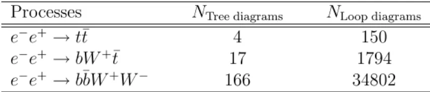
The complexities will be increased tremendously when one calculates the multi- particles processes possessing the following problems. The first complicated issue is related to handing a huge number of Feynman diagrams. For example, several 2 → 2, 3 and 4 processes at the ILC are considered at the level of one-loop corrections. The number of Feynman diagrams in the covariant gauge are listed in Table 2.1. One finds that the number of Feynman diagrams raise tremendously with increasing number of final particles.

Processes NTree diagrams NLoop diagrams

e⁻e⁺_{→ t¯t} 4 150

e⁻e⁺_{→ bW}⁺t^¯ 17 1794

e⁻e⁺_{→ b¯bW}⁺W⁻ 166 34802

Table 2.1: The number of Feynman diagrams in the covariant gauge. NLoop diagrams

includes one-loop virtual diagrams and counterterm diagrams.

The strategy for hand calculation of these processes is to select the dominant diagrams. The diagrams contained the coupling of Higgs to electron and position, for example, can be omitted, because their contributions are smaller than the Monte Carlo integration accuracy. However, the hand calculations are very difficult to per- form and prone to error. Furthermore, a complete hand calculation for such processes is impossible. Even in the tree level, the integration the squared total amplitude of the given process is impossible to evaluate by hand calculation.

Beside handing huge number of Feynman diagrams, the technique for evaluating

tensor one-loop and two-loop integrals is very complicated. There are no ideal tech- niques up to now for complete tensor two-loop integrals with arbitrary internal masses in analytical manner. The tensor one-loop integrals up to six point functions were performed by several approaches. In general, the tensor integrals will be reduced into the basic scalar integrals which are scalar one-loop one-, two-, three- and four-point functions. The difficulties in the evaluation of tensor one-loop integrals are to deal with a Gram determinant problems, Landau singularity [31]. The Landau singularity is related to the appearance of unstable particles.

The traditional method for tensor one-loop reduction was proposed by Passarino and Veltman [15]. In this scheme, the tensor integrals were decomposed into the Lorentz-covariant structure with coefficient of the form factor integrals which later written in terms of the scalar integrals. By contracting the Minkowski metric (gµν) and external momenta into the tensor integrals, one can obtain the form factors. In this step, we have to solve a system of linear equations where the Gram determinants appear in the denominator. If the Gram determinants will vanish or become very small, the reduction method will break or spoil numerical stability.

In Ref [16], numerically stable reduction for tensor one-loop integrals up to six points was introduced. In this method the modified Caylay determinants are used to avoid zero Gram determinants. For the cases where Gram determinants become very small, suitable expansions are employed in order to gain the numerically stable results. The method was applied successfully to calculate e⁻e⁺ → 4 fermions processes in Refs [17, 18, 19].

In addition, the on-shell methods have been developed in Refs [22, 23]. The methods are analytical one which differs from PV. In progress, the on-shell methods have been mainly applied to calculate one-loop multi-leg QCD processes. It can be extended for the massive cases which can hence be used for electroweak processes. In the on-shell method the Gram determinant problems have not been solved completely but it can be under control.

2.2. Introduction to GRACE-Loop ₁₅

A semi-analytical method for reduction of tensor one-loop integrals which can overcome Gram determinant problems, was presented in Refs [24, 25, 26]. In the same progress with the on-shell method, the semi-analytical method has been mainly applied to calculate one-loop multi-leg QCD processes.

A reduction method in Feynman-parameters space, the improved Brown-Feynman reduction method, has been used in GRACE-Loop [21]. This method will be discussed in further detail in the next section.

Faced with these difficulties, an ideal solution for automatic calcula- tions of multi-particle processes including radiative corrections from the Lagrangian, is proposed. For the purpose, the thesis will introduce and focus on development of the GRACE-Loop program.

2.2 Introduction to GRACE-Loop

GRACE is a generic automatic computer program for calculating High Energy Physics processes up to one-loop corrections within the SM and Minimum Super-Symmetry Model (MSSM) [32]. The program has been developed by MINAMI-TATEYA group at High Energy Accelerator Research Organization (KEK) [33] and at some universi- ties¹. The first version of GRACE is dedicated to GRACE-tree which provides helicity amplitude and corresponding cross section at tree level. This version includes the SM and MSSM as well as many other BSMs.

GRACE-Loop has been then developed in 2002 [21]. It mainly focuses on the one-loop electroweak corrections to the SM processes at e⁺e⁻ colliders. In parallel with the GRACE-Loop development, the program named GRACE-SUSY/1-LOOP has also been built for evaluating one-loop corrections in the MSSM [34, 35, 36]. This thesis only focuses on describing the GRACE-Loop program. The feature of the program and its structure will be presented in the next paragraphs.

1Kogakuin, Seikei, Chiba, Meiji Gakuin universities and Tokyo Management College.

In the GRACE-Loop, the renormalization is carried out with the on-shell renor- malization conditions of the Kyoto scheme, as described in Ref [37]. The ultraviolet (UV) divergences are regulated by dimensional regularization, while the infrared (IR) divergences are regularized by giving the virtual photon an infinitesimal mass λ. It will be described in more detail in the next sections.

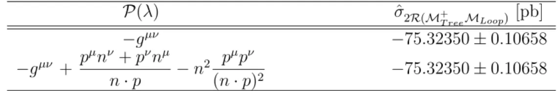
The program has been equipped with so-called non-linear gauge fixing terms [38] in the Lagrangian which are described in Eq.(1.17). In the practical calculation, we are working in the Rξ-type gauges with the condition ξW = ξZ = ξA = 1 (also called the ’t Hooft-Feynman gauge). There is no longitudinal contribution in the gauge propagator. This choice has not only the advantage of making the expressions much simpler. It also avoids unnecessary large cancellations, high tensor ranks in the one-loop integrals and extra powers of momenta in the denominators which cannot be handled by the FF and LoopTools packages [39, 40]. With the implementation of non-linear gauge fixing terms the program provides a powerful tool to check the results in a consistent way. After all, the results must be independent of the non- linear gauge parameters. It will be discussed in greater detail in chapter 3, section of test on the calculation of pp → W^+W−+ 1 jet at the LHC.

In its latest version GRACE-Loop can use the axial gauge in the pro- jection operator for external photons. This implementation is achieved in this thesis. It cures a problem with large numerical cancellations. This is very useful once calculating processes at small angle and energy cuts for the final particles. This implementation also provides a useful tool to check the consistency of the results which, due to the Ward identities, must be independent of the choice of the gauge.

The structure of GRACE-Loop is described in the following flow chart 2.1. Its structure is also explained explicitly in the following paragraphs:

ˆ THEORY: the SM model with non-linear gauge fixing terms in the Lagrangian

2.2. Introduction to GRACE-Loop ₁₇

U S E R S

( p a r t i c l e s , o r d e r , e t c )

T H E O R Y ( M o d e l f i l e )

D i a g r a m s g e n e r a t o r D r a w e r

(eps, ps files)

M a t r i x E l e m e n t G e n e r a t o r ( FORM source code)

G e n e r a t e d F O R T R A N k i n e m a t i c s

C o d e

L o o p T o o l s o r F F ;

H o m e m a d e

BASES

M o n t e C a r l o I n t e g r a t i o n

P a r a m e t e r F i l e

S P R I N G

E v e n t G e n e r a t o r

E v e n t s

C r o s s s e c t i o n R e l a v e n t D i s t r i b u t i o n s

M P I

C o d e

Figure 2.1: The GRACE-Loop flow chart.