PDF University of the Ryukyus

ISSN   2434-6071

RYUKYU MATHEMATICAL JOURNAL

VOL. 31

2018

DEPARTMENT OF MATHEMATICAL SCIENCES, FACULTY OF SCIENCE

RYUKYU MATHEMATICAL JOURNAL VOL. 31, 2018

CONTENTS

Y. HASHIMOTO, On the security of Zhang-Tan’s variants of multivariate signature schemes

. . . 1 T. SUDO, A locally commentative, deformative learning in the

arithmetic noncommutative geometry as flower gardening

variation . . . 7

ON THE SECURITY OF ZHANG-TAN’S VARIANTS OF MULTIVARIATE SIGNATURE SCHEMES ∗

Yasufumi HASHIMOTO

Abstract

Until now, various multivariate public key cryptosystems (MPKCs) have been proposed but some of them are known to be insecure. In IMACC 2015 and Inscrypt 2015, Zhang and Tan proposed new variants of MPKCs for signatures to enhance the security of the original schemes. However, Zhang-Tan’s variants are much less secure than expected. In this paper, we describe an attack on Zhang-Tan’s variants to recover a public key of the original scheme.

1 Introduction

After Shor [6] proposed polynomial-time algorithms to factor integers and to solve discrete logarithm problems by quantum computers, constructing cryptosystems secure against quantum attacks is one of big issues in cryptology.

sets of multivariate quadratic forms over finite fields, have been expected to be such cryptosystems. While various MPKCs have been proposed until now, some of them were broken soon after proposed or known to be much less secure than expected.

In IMACC 2015 and Inscrypt 2015, Zhang and Tan [9, 10] proposed a new idea to repair such insecure MPKCs for signatures. Their idea is adding several variables and terms for the additional variables on the original polynomials, and hiding several equations to eliminate the contributions of additional variables in the process of signature generation. They actually used this idea on already broken schemes MI- T [8] and YTS [7, 2] by adding HFE-like polynomials and claimed that this idea enhanced the security drastically. However, the hidden equations can be recovered by sufficiently many signatures and these equations tell us partial information of the secret key. In this paper, we describe how to recover the hidden equations and the secret key partially, and conclude that our attack removes the contributions of the additional variables and recovers a public key of the original scheme.

Ryukyu Math. J., 31(2018), 1-5

2 Multivariate Public Key Cryptosystem

In this section, we describe the general construction of multivariate public key cryp- tosystems (MPKCs).

Let

1 be integers,

a finite field and

:= #k. Define a quadratic map

:

to be inverted feasibly, i.e. finding

with

is feasible for any (or most)

. The

is a tuple of three maps (S, G, T ), where

:

,

:

are invertible affine maps and the quadratic map

:

. The

is the convolution of these three maps

F

:=

:

On an encryption scheme, the

for a given plain-text

is computed by

=

(x). To

with

(y). Then the plain-text is

=

(z). Since

is constructed to be inverted feasibly, one can decrypt

feasibly.

On a signature scheme, a signature

for a given message

is generated as follows. Find

with

and compute

=

(z). The signature

for

is verified if

=

3 Zhang-Tan’s variant

In this section, we describe Zhang-Tan’s variant [9, 10] on MPKC.

Let

1 be integers with

=

+

and

=

(x

),

=

t

(x

),

=

(x

) are variables. Define the quadratic maps

:

,

:

by

G(x) =^t

(g

(x), . . . , g

(x)),

(h

(x), . . . , h

(x)), where

(x), . . . , g

(x) are quadratic forms of

and

h_i

(x) =(homogeneous quadratic form of

)

+

1≤j≤l

x_n0+j ·

(linear form of

), (1

(1)

Suppose that

are inverted feasibly, i.e. finding

with

) =

is feasible for any (or most)

and finding

with

) = 0 is also feasible for any (or most)

. In [9, 10],

is the central map of MI-T [8] or YTS [7] and

is given by an HFE-like polynomial.

Zhang-Tan’s variant is given as follows.

Secret key.

Two invertible affine maps

:

,

:

, a linear map

:

and the quadratic maps

:

,

:

defined above.

Public key.

The quadratic map

:

defined by

:= (T

+

Signature generation.

For a message

to be signed, find

with

) =

(y), and

with

) = 0. The signature is

=

(z

).

Signature verification.

The signature

is verified if

(w) =

holds.

Since

and is constructed to be inverted feasibly,

is found feasibly. Similarly, finding

is also feasible. Note that

is constructed such that

0) = 0 for any

. Then

= 0 is acceptable in the process of signature generation if there are no non-trivial

for a given

.

4 On the security of Zhang-Tan’s variant

In this section, we propose our attack to reduce the problem of solving

(x) =

to the problem of solving

(x

) =

where

:=

is a public key of the original scheme derived from

:

is an invertible affine map.

For simplicity, we assume that

is a linear map.

First, recall that one finds

with

) = 0 in the process of signature generation, and the signature

satisfies (z

) =

holds for any signature

generated by the corresponding Zhang-Tan’s variant.

This means that there are

(x), . . . , u

(x) with

(w) = 0 for any signature

and these quadratic forms are linear sums of

(S(x)), . . . , h

(S(x)). Since

is a quadratic form of

variables, we can recover

(x), . . . , u

(x) by

+ 1) signatures.

By the construction (1) of

(x) are written by

(x) =

0

∗ ∗l

Sx

+ (linear form)

for 1

This is similar to the quadratic form in UOV [5, 3] and then, once

(x), . . . , u

(x) are given, the attacker can recover an invertible linear map

:

with

=

∗n0 ∗

0

by Kipnis-Shamir’s attack on UOV [4, 3] in time

(polyn.)).

Since ¯

:=

= (T

+

(S

) and

=

S₀ ∗

0

with

some

matrix

, we see that

(S

) is a set of quadratic forms as

given in (1). Then we have ¯

(x

0) = (T

)(x

), which is a public key of the

Step 1.

Let

be an integer sufficiently larger than

+ 1). Choose

mes- sages

randomly, and generate signatures

for

respectively.

Step 2.

Find

linearly independent quadratic forms

(x), . . . , u

(x) with

(w

) = 0 for any 1

.

Step 3.

Find an invertible linear map

:

with

(S

(x)) =

0

∗ ∗_l

x

+ (linear form) for 1

by Kipnis-Shamir’s attack [4, 3].

Step 4.

Let ¯

:=

Then ¯

(x

0) is a public key of the original scheme.

As already explained, the complexity of Step 3 is

(polyn.)). It is easy to see that the complexities of other steps of our attack are in polynomial time. Then the total complexity of our attack is

(polyn.)), which is much less than

(polyn.)) expected by Zhang and Tan [9, 10]. This means that

must be sufficiently larger than

, namely the number

of variables in Zhang- Tan’s variant must be sufficiently larger than twice of the number

of the variables in the original scheme. This situation is similar to UOV [3], and we can consider that Zhang-Tan’s variant does not have an advantage over UOV. Furthermore, the complexity

(polyn.)) might be improved if

has a special structure.

For example, when

is given by an HFE-like polynomial [9, 10], the rank attack [1] will reduce the complexity. We thus conclude that Zhang-Tan’s variant is not practical at all.

Acknowledgment.

This work was supported by JST CREST Grant Number JP- MJCR14D6 and JSPS Grant-in-Aid for Scientific Research (C) no. 17K05181.

References

[1]

L. Bettale, J.C. Faugere, L. Perret, Cryptanalysis of HFE, multi-HFE and variants for odd and even characteristic, Designs, Codes and Cryptography

(2013), pp.1-52.

[2]

Y. Hashimoto, Cryptanalysis of the multivariate signature scheme proposed in PQCrypto 2013, PQCrypto’14, LNCS

(2014), pp.108–125, IEICE Trans.

Fundamentals,

(2016), pp.58–65.

[3]

A. Kipnis, J. Patarin, L. Goubin, Unbalanced oil and vinegar signature

schemes, Eurocrypt’99, LNCS

(1999), pp.206–222, extended in cite-

seer/231623.html, 2003-06-11.

[5]

J. Patarin, The Oil and Vinegar Signature Scheme, the Dagstuhl Workshop on Cryptography, 1997.

[6]

P.W. Shor, Polynomial-time algorithms for prime factorization and discrete logarithms on a quantum computer, SIAM J. Computing

(1997), pp.1484–

1509.

[7]

T. Yasuda, T. Takagi, K. Sakurai, Multivariate signature scheme using quadratic forms. PQCrypto’13, LNCS

(2013), pp.243–258.

[8]

W. Zhang, C.H. Tan, A new perturbed Matsumoto-Imai signature scheme, AsiaPKC’14, Proc. 2nd ACM Workshop on AsiaPKC (2014), pp.43–48.

[9]

W. Zhang, C.H. Tan, MI-T-HFE, A new multivariate signature scheme, IMACC’15, LNCS

[10]

W. Zhang, C.H. Tan, A secure variant of Yasuda, Takagi and Sakurai’s signature scheme, Inscrypt’15, LNCS

(2015), pp.75-89

Department of Mathematical Sciences Faculty of Science

University of the Ryukyus

Nishihara-cho, Okinawa 903-0213

JAPAN

A locally commentative, deformative learning in the arithmetic

noncommutative geometry as flower gardening variation

Takahiro Sudo

Dedicated to Professor Takashi Ito on his 60th birthday with gratitude and respect

Abstract

We would like to study noncommmutative geometry, related to Arith- metics in some sense. For this purpose forced, we review and study the lecture notes by Marcolli, on the arithmetic noncommutative geometry.

MSC 2010: Primary 46-01, 46-02, 46L05, 46L51, 46L53, 46L55, 46L80, 46L85, 46L87, 46L89, 19K14, 19K56, 81Q10, 81Q35, 81R15, 81R40, 81R60, 81T75, 11G18, 11M06, 11R37, 11R42.

Keywords: Noncommutative geometry, C*-algebra, K-theory, spectral triple, zeta function, modular group, modular curve, quantum statistical mechanics, Bost-Connes system, KMS state, class field theory, Schottky, hyperbolic, arith- metic, archimedean, Arakelov geometry, Green function, black hole, L-function, L-factor, algebraic variety, Shimura variety, Cuntz-Krieger algebra.

1 Overture

Preface. Just following, almost along the story of Matilde Marcolli [114], as nothing but a running commentary, as purpose of background learning, we (as beginners) would like to study what is growing and harvested (at that time) on the rathermysterious noncommutative world (as a vast field), related to Arith- metics, as a back to the past for a return to the future (BPRF) flower gardening variation as named. All necessary things are to be considered until the end is to be watched. Our local understanding the details (in part) may be shallow or somewhat limited. With some considerable effort within the time limited for publication, we would like tomake some additional or deformed, comments, corrections, descriptions, (partial) proofs, or remarks, on the contents, to be or not to be self-contained.

Received November 30, 2018.

Ryukyu Math. J., 31(2018), 7-164

In particular, as a note we use the symbols · · · (texts) as indicating either personal comments, computations to be checked, or etc. As well, some additional remarks starting with Remark· · · (texts) in the text below are alsomade fromsuitable related references to be included. All the details could not be contained in these cases. Some notations as well as style are (slightly) changed fromthe original ones by our taste. As usual, leti=√

−1. Denote by Q,R, andCthe fields of rational, real, and complex numbers, respectively.

Once upon a time and space, there is certainly or simply, a sort of synchro- nized improvement based on the achievement of Marcolli, like a decorated field on the high splended hill. The variant flower garden is now open!

Table 1: Contents♣ Section& Subsection

1 Overture

1.1 The space-algebra-geometry dictionary 1.2 Noncommutative spaces encountered

1.3 Spectral triples appeared 1.4 Why NCG?

2 Noncommutativemodular curves 2.1 Modular curves

2.2 The noncommutative boundary ofmodular curves 2.3 Limitingmodular symbols

2.4 Hecke eigenforms 2.5 Selberg zeta function

2.6 Themodular complex and K-theory ofC^∗-algebras 2.7 Chaotic cosmology asIntermezzo

3 Quantum statistical mechanics and Galois theory 3.1 Quantumstatisticalmechanics

3.2 The Bost-Connes system

3.3 Noncommutative geometry and the Hilbert 12th problem 3.4 TheGL2 system

3.5 Quadratic fields

4 Noncommutative geometry at arithmetic infinity 4.1 Schottky uniformization

4.2 Dynamics and noncommutative geometry 4.3 Arithmetic infinity as archimedean primes 4.4 Arakelov geometry and hyperbolic geometry 4.5 Qunatum gravity and black holes asIntermezzo

4.6 Dual graph and noncommutative geometry 4.7 Arithmetic varieties andL-factors

4.8 Archimedean cohomology 5 The vista around

References

Section 1. Let us start by recalling several preliminary notions of noncom- mutative geometry, following Connes [27].

Section 2. Let us describe how various arithmetice properties ofmodular curves can be viewed as their noncommutative boundaries as noncommutative spaces or algebras. Themain references are Manin-Marcolli [112] and Marcolli [113], [115].

Section 3. This section includes an account of the work of Connes and Marcolli [41] on the noncommutative geometry for commensurability classes of Q-lattices. Also included is the relation of the noncommutative geometry for these classes to the Hilbert 12th problem of explicit class field theory as well as the results of Connes, Marcolli, and Ramachandran [48] on the construction of a quantumstatisticalmechanical systemthat recovers the explicit class field theory of imaginary quadratic fields. As well, included is a brief explanation on the real multiplication program of Manin [109], [110] and the problem of real quadratic fields.

Section 4. This section contains the noncommutative geometry for the fibers at arithmetic infinity of varieties over number fields, based on Consani and Marcolli [58], [59], [60], [61], [63]. Also contained is a detailed account of the formula of Manin for the Green function of Arakelov geometry for arithmetic surfaces, based on Manin [106] as well as a proposed physical interpretation of this formula, as in Manin and Marcolli [111].

Noncommutative geometry (NG) is developed by Connes, started in the early 1989s as in [22], [24], [27]. The NG extends tools of ordinary geometry to treat spaces obtained as certain quotients by some equivalence relations, for which the usual ring of functions on quotients defined as functions invariant with respect to the equivalence relation becomes too trivial to capture the information on the structure of points of the quotient space, and so to define a noncommuta- tive algebra or space with generators corresponding to coordinates of the space, remembering the structure of the equivalence relation, and analogous to non- commuting variables in quantum mechanics. These quantum spaces defined so extend the Gel’fand -Naimark correspondence between locally compact, Haus- dorff spaces and commutative C^∗-algebras of all continuous, complex-valued functions on the spaces (vanishing at infinity) by dropping the commutativity hypothesis. Namely, a noncommutative (NC) (topological) space is defined to be a noncommutativeC^∗-algebra.

Such quotient spaces are abundant in nature. For instance, they arise by foliations as equivalence relations. As well, noncommutative spaces arise natu- rally in number theory and arithmetic geometry. The first connection between noncommutative geometry and number theory is obtained by Bost and Connes [13], in which exhibited is an interesting noncommutative space or algebra with remarkable arithmetic properties related to the class field theory. This also in- volves the phenomena as spontaneous symmetry breaking in quantumstatistical mechanics related to the Galois theory. That space can be viewed as the NC space of 1-dimensional Q-lattices up to scale,modulo the equivalence relation of commensurability (Connes-Marcolli [41]). As well, the NC space is closely

related to the noncommutative space by Connes [29] to obtain a spectral real- ization of zeros of the Riemann zeta function. In fact, this NC space is that of commensurability classes of 1-dimensional Q-lattices, but with the scale factor also taken into account.

The deeper connections between noncommutative geometry and number the- ory are obtained by Connes and Moscovici [54], [55] on the modular Hecke al- gebras. It is shown that the Rankin-Cohen brackets as an important algebraic structure onmodular forms (Zagier [159]) have a natural interpretation in terms of the Hopf algebra of the transverse geometry of foliations with codimension 1, in the sense of NG. Themodular Hecke algebras, in which products and action of Hecke operators on modular forms are naturally combined, can be viewed as the holomorphic part of the NC algebra of coordinates on the space of com- mensurability classes of 2-dimensional Q-lattices, constructed by Connes and Marcolli [41].

On the other hand, the classification of noncommutative 3-spheres is ob- tained by Connes and Dubois-Violette [35], [36], [37], in which the corresponding moduli space has a ramified cover by a noncommutative nilmanifold, where the NC analog of the Jacobian of this coveringmap is expressed naturally in terms of the Dedekind eta function, as an interesting case of number theory within NG. As another such case, calculated by Connes [31] the explicit cyclic cohomol- ogy Chern character of a spectral triple onSUq(2), also defined by Chakraborty and Pal [17].

More other instances of NG spaces that arise in the context of number theory and arithmetic geometry can be found in the noncommutative compactification of modular curves, as Connes, Douglas, and Schwarz [34], Manin and Marcolli [112]. This NC space is again related to the NG of Q-lattices. In fact, it can be seen as a stratum in the compactification of the space of commensurability classes of 2-dimensionalQ-lattices (CM [41]).

Another context in which NG provides a useful tool for arithmetic geometry is given by the description of the totally degenerate fibers at arithmetic infinity of arithmetic varieties over number fields, analyzed by Katia Consani and Marcolli [58], [59], [60], [61].

The present text is based on the lecture notes [114] on the lectures given by Marcolli, in 2002 to 2004,may be used later on.

In the lectures, contained as themain focus is the noncommutative geome- try of modular curves (MM [112]) and of the archimedean fibers of arithmetic varieties ([61]). Also included is a theory of the NG space of commensurability classes of 2-dimensionalQ-lattices ([41]). In particular, conveyed is the general picture less than the details of the proofs of the specific results. Though proof are almost not included in the (original) text, the readermay find references to the relevant literature, such as [41], [48], [61], and [112].

From the foreword by Manin as backward. (Edited, changed for short.) Let us be imagining C^∗-algebras as coordinate rings, and making bridges to commutative geometry via crossed products ofC^∗-algebras, to involve noncom- mutative Riemannian geometry, with algebraic tools as K-theory and cyclic

cohomology for C^∗-algebras and their subalgebras.

Let us be studying various aspects of uniformization by the classicalmodu- lar group as well as Schottky groups. Themodular group acts on the complex half plane, partially compactified by cusps as rational points of the boundary projective line overC. The action at irrational points is viewed as the noncom- mutative boundary as NC spaces, entering NG. Moreover, as contentsmentioned as follows:

Schottky uniformization provides a visualization of Arakelov geometry at arithmetic infinity.

Gauss characterising regular polygons that can be constructed using only ruler and compass.

In the complex plane, roots of unity of degreenformvertices of a regular n-gon.

Being constructible as themaximal Galois extensionQofQ, to calculate the Galois group Gal(Q/Q).

Gauss Galois group Gal^Ab(Q/Q) in Bost-Connes symmetry breaking and Gauss statistics of continued fractions in the chaotic cosmologymodels.

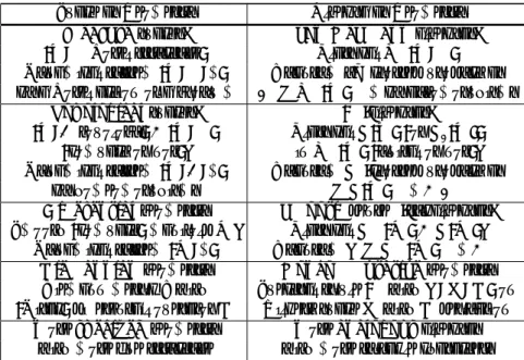
1.1 The space-algebra-geometry dictionary

There is a dictionary relating concepts of ordinary geometry to the correspond- ing counterperts in noncommutative geometry (cf. [27] as well as [154]).

Table 2: The S-A-G overview dictionary, as translated Space as Geometry Algebra as Geometry

Measurespaces: von Neumann algebras:

(X,BBorel structure) ClassicalL^∞(X,B) Dynamical system(X,B,Γ) QuantumvN crossed product as by a Borel action of a group Γ M=L^∞(X)Γ by automorphisms

Topologicalspaces: C^∗-algebras:

(X,Otopology)⊂(X,B) ClassicalC(X) (orC0(X)) (compact or not); inL^∞(X) (unital or not);

Dynamical system (X,O,Γ) QuantumC^∗-crossed product as

by homeomorphisms A=C(X)Γ⊂M

Differential geometry Smoothdense∗-subalgebras:

Smooth (compact)manifoldM; ClassicalC^∞(M)⊂C(M);

Dynamical system(M,Γ) QuantumA=C^∞(M)Γ⊂A Riemanniangeometry Noncommutativegeometry

Riemannmetricdwith Spectral triple (AwithA,H,D) on (Dirac) differentail operator D Hilbert spaceH withD derivation

Morespecifiedgeometry Moreanalogousalgebras withmore fine structure withmore suitable characters

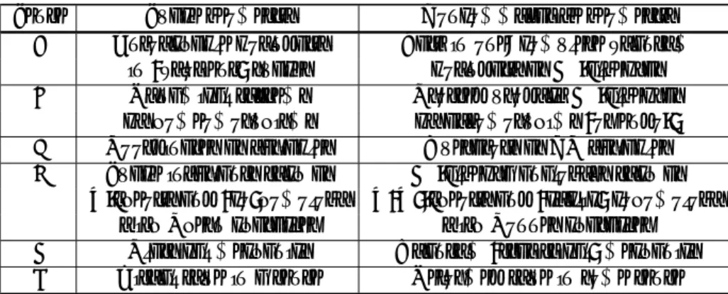
1.2 Noncommutative spaces encountered

The way to assign the algebra of coordinates to a quotient spaceX =Y /∼of a spaceY by an equivalence relation ∼may be explained as follows.

• One way to consider functionsf onY withf(a) =f(b) fora∼b inY. If each equivalence class as a subset ofY is dense inY and iffis continuous onY and constantc on an equivalence class, thenf ≡c1 on Y.

•The other way to consider functions on the graph of the equivalence rela- tion.

A noncommutative algebra is obtained by the second description, with a convolution product determined by the groupoid law of the equivalence relation, like the usual product of theC^∗-algebra ofn×nmatrices overCas

f∗g=f g=

⎛

⎜⎝

f11 · · · f1n

... . .. ... f1n · · · fnn

⎞

⎟⎠(gij)ⁿ_i,j=1 = ( n k=1

fikgkj)ⁿ_i,j=1∈Mn(C).

Even though the two functional notions for quotients are not the same, but they may be related by Morita equivalence, as a suitable notion as a (stable) isomorphism between NC spaces. However, the second notion is the only one to allow tomake sense of (NC) geometry for the general quotient spaces.

Example 1.1. Refer to [30]. LetY = [0,1]×{0,1}with the equivalence relation as points (x,0)∼(x,1) for anyx∈(0,1) the open interval. ThenX=Y /∼is identified with a topological union with the quotient topology as

{(0,0),(0,1)} ∪(0,1)∪ {(1,0),(0,1)}.

The first way implies C([0,1]) (not C, corrected), but the commutative C^∗- algebra of all continuous, complex-valued functions on the closed interval [0,1].

On the other hand, the second way implies the continuous C^∗-algebra bundle over [0,1] with fibers M2(C) on (0,1) andC² at 0 and 1, which can be written as aC^∗-algebra extensionE as a NC algebra

0→SM2(C) =C0((0,1))⊗M2(C)→E→C²⊕C²→0, where eachC²is identified with the diagonal part of M2(C).

Note that there is analogy between the idea of preserving the informa- tion of the equivalence relation in the description of quotient spaces and the Grothendieck theory of stacks in algebraic geometry.

Morita equivalence. In NC geometry, the proper notion as isomorphisms of C^∗-algebras is provided by Morita equivalence of C^∗-algebras, or (equivalent) their stable isomorphisms. Namely, for (separable)C^∗-algebrasAand B, they arestably isomorphic ifA⊗K∼=B⊗K, whereK=K(H) is theC^∗-algebras of all compact operators on a (separable) Hilbert space H.

C^∗-algebras A and B are (strongly) Morita equivalent if there is a A-B bimoduleM, which is a left HilbertA-module with anA-valued inner product

·,·A, and is a right HilbertB-module with anB-valued inner product·,·B, such that (corrected)

(1) A=M,M_A and B=M,M_B, (2) ξ1, ξ2Aξ3=ξ1ξ2, ξ3B, ξ1, ξ2, ξ3∈M,

(3) aξ, aξ_B≤ a²ξ, ξ_B, ξb, ξb_A≤ b²ξ, ξ_A,

fora∈A, b∈B, ξ∈M, so that Aand Bact onMfromthe left and right, as bounded operators.

Wemay assume thatM=ACBfor aC^∗-algebraCsuch that ACA⊂A⊂C and BCB⊂B⊂C.

Then AM⊂MandMB⊂M. Also, wemay assume thatx, y_A=xy^∗ ∈A andx, y_B=x^∗y∈Bforx, y∈M. Because

ACBB^∗C^∗A^∗⊂MM^∗⊂A and B^∗C^∗A^∗ACB⊂M^∗M⊂B.

Then, for anyx, y, z∈M,

x, y_Az=xy^∗z=xy, z_B. As well, for anya∈A, b∈B, ξ∈M,

aξ, aξB=ξ^∗a^∗aξ≤ξ^∗a^∗a1ξ=a²ξ, ξB inB+, ξb, ξbA=ξbb^∗ξ^∗≤ξbb^∗1ξ^∗=b²ξ, ξA, in A+. For instance, wemay let

ACB≡

A 0

0 0

C C

C C 0 0 0 B

=

0 ACB ≡M

0 0

≡M.

Then

MM^∗ =

M(M)^∗ 0

0 0

⊂A and M^∗M=

0 0 0 (M)^∗M

⊂B.

This picture quite explains the meaning of Morita equivalence. Namely the triangle corners!

In particular,C∼=C⊕0n =A andMn(C) ∼= 0⊕Mn(C) =B as diagonal sums inMn+1(C) are Morita equivalent since

ACB= (C⊕0n)Mn+1(C)(0⊕Mn(C))

=

C 0 0 0n

C Cⁿ

(Cⁿ)^t Mn(C) 0 0 0 Mn(C)

=

0 Cⁿ 0 0n

=M,

MM^∗∼=Cⁿ(Cⁿ)^t∼=C and M^∗M∼= (Cⁿ)^∗Cⁿ ∼=Mn(C), withCⁿ as a row vector space and (Cⁿ)^tas a column vector space.

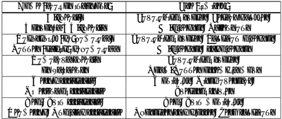
The tools de noncommutative geometry.

Table 3: The tool box

Name (tool as invariant) Use (limited)

K-theory, Topological spaces, Vector bundles, Kasparov KK-theory C^∗-algebras, Extensions Hochschild (co)homology, Topological spaces, Function algebras, Connes (cyclic) cohomology C^∗-algebras, subalgebras

Homotopy theory Topological spaces,

as quotients Baum-Connes assembly maps Metric structure, Manifolds, Dirac operator, Differential structure Spectral triples Real, Spin structure, Real, Spin manifolds,

Geometric, Analytic structure Characteristic classes, Zeta functions

As an important note, please handle these tools with the greatest care!

1.3 Spectral triples appeared

We are going to take a (moment) look at the analogue in the NC world of Riemann geometry, provided by Connes. Spectral triples as a generalization of the structure of a Riemannianmanifold play a crucial role in noncommutative geometry. In the usual context of Riemann geometry, the definition of the infinitesimal elementdson a smooth spinmanifold can be expressed in terms of the inverseD⁻¹of the classical Dirac operatorD. The theory of spectral triples (ST) is motivated by this key remark. In particular, the geodesic distance between two points of themanifold is defined in terms ofD⁻¹ (cf. [27, VI]).

Example 1.2. (Added). The geodesicdistance formula for a Riemann spin manifoldM is given by

d(x, y) = sup{|f(x)−f(y)|f ∈C^∞(M),[D, f] ≤1},

whereD is theDiracoperator, defined as _ds^d, so that [D, f] =MDf themulti- plication operator on the Hilbert spaceL²(M), because

[D, f]g= [D, Mf]g= (DMf−MfD)g

=D(f g)−f Dg

= (Df)g+f Dg−f Dg=MDfg, f, g∈C^∞(M), andC^∞(M) is dense inL²(M). For more details,may refer to [150].

The triple

(C(M), L²(M), D= d ds)

is the typical example of spectral triples in the commutavie case. Indeed, the C^∗-algebra C(M) of all continuous, complex-valued functions on a compact (Riemann spin) manifold M contains the norm dense∗-subalgebraC^∞(M) of all smooth differentiable functions onM, on which as a dense domain inC(M), the (Dirac) differential operator _ds^d is certainly defined. The representation of C(M) onL²(M) is given asmultiplication operators.

As a generalization of the commutative case to the noncommutative case, given by Connes is the following (cf. [27], [28], [50]):

Definition 1.3. A (Connes) spectral triple(SpTr) is defined to be a triple (A, H, D) of a C^∗-algebra A, a C^∗-algebra representation ρ : A → B(H) the C^∗-algebra of all bounded operators on a separable Hilbert space H, and a (unbounded, Dirac) operatorD, such that

(1)D=D^∗ as self-adjointness, with its spectrumin R.

(2) For anyλ∈R, the resolvent (inverse) operator (D−λ1)⁻¹is a compact operator onH.

(3) For any a ∈ A = A^∞ a dense involutive (or ∗-) subalgebra A, the commutator [D, ρ(a)] is a bounded operator onH.

Remark. (Edited). The above property (2) can be regarded as a generalization of the ellipticity property of the standard Dirac operator on a compactmanifold.

In the classical case of Riemannmanifolds, the property (3) is equivalent to the Lipschitz condition, which is weaker than the smoothness condition.

Indeed, the geodesic distance formula forM is converted as theLipschitz normforf ∈C^∞(M) as

L(f)≡ sup

x=y∈M

|f(x)−f(y)|

d(x, y) =df

ds∞=MDf=[D, f].

Then the boundedness of L(f) with f_∞ ≤ 1 is equivalent to that of the operator [D,·].

The basic geometric structure encoded by the theory of spectral triples is Riemann geometry. But in more refined cases such as K¨ahler geometry, the additional structure can be encoded as additional symmetries. For instance, in the case where the algebra involves the action of the Lefschetz operator of a compact K¨ahler manifold, can be encoded the information on the K¨ahler form, at the cohomological level (cf. [61], [63]).

As the relations among NG, arithmetic geometry (AG) and number theory (NT), the interesting feature of spectral triples (SpTr) is that we have an as- sociated family of zeta functions (defined as the trace for the operator |D|^−z) and the theory of volumes and integration, which is related to special values of these zeta functions.

Volume form. Based on [27], [28]. May refer to [150] as well. A Connes spectral triple (A, H, D) is said to ben-summable, or of dimensionnif|D|⁻ⁿ is an infinitesimal (or a compact operator) of order one, in the sense that the eigenvalues λk(|D|⁻ⁿ) of|D|⁻ⁿ satisfy the estimateλk(|D|⁻ⁿ) =O(k⁻¹) (k→

∞), whichmeans 0≤λk(|D|⁻ⁿ)≤ ^M_k for some constantM >0 and anyklarge enough.

Consider a positive compact operatorT with decreasing eigenvaluesλj(T)≥ 0 with multiplicities counted such that k−1

j=0λj(T) = O(logk) (k → ∞) as a (logarithmic) divergence, equivalently, with the sequence boundedenss

1 logk

k−1

j=0λj(T) ≤ M for some M > 0 and any k large enough, as the (in- verse) logarithmic (possible) divergence. The Dixmier trace trω(T) of such T ∈L^1,∞(H)⊂B(H), containing atraceclass operatorT ∈L¹(H) such that

T1= tr(|T|) = ∞ j=0

λj(|T|)<∞, is defined to be

trω(T) = lim

ω

1 logk

k−1

j=0

λj(T)≡ω({ 1 logk

k−1

j=0

λj(T)}k),

whereω is a certainly chosen functional inC^b(N)^∗ the dual space ofC^b(N) the C^∗-algebra of all bounded complex sequences, with several properties, extending the usual limit for convergent sequences.

Namely, lim≤limω=ω as the limit extension. Note that functionals (on NC spaces or algebras) are viewed as (noncommutative) integrations.

The Dixmier trace is also defined on compact operators with order one as infinitesimals.

The reason for this is implied by that theEulerconstantγ as the limit

klim→∞(1 +1

2 +· · ·+1

k−logk) =γ exists, with ¹₂ ≤γ <1.

An operatorT in the definition domain of the Dixmier trace(s) is said to be measurable if the D-trace trω(T) does not depend on the choice of the limit functionalω= limω.

The operator|D|⁻ⁿ on a noncommutative spaceAgeneralizes the notion of a volume form on a usual space. The (noncommutative) (total)volumeforA orA(n-summable) is defined to be

V = trω(|D|⁻ⁿ)≡ |A|or|A|.

More generally, for an element aof the algebra D generated by Aand [D,A], its (normalized)integrationwith respect to the volume form|D|⁻ⁿ is defined

as 1

V

a= 1

Vtrω(a|D|⁻ⁿ).

The usual notion of integration on a Riemann spin manifold M can be revovered in this context by the formula

M

f dv= 2^n−[n2]−1πⁿ²nΓ(n

2)trω(Mf|D|⁻ⁿ),

where D is the classical Dirac operator on M associated to the metric that determines the volume form dv, and Mf is the multiplication operator acting on the Hilbert space of all square integrable (L²) spinors (or sections of a certain bundle) onM (cf. [27], [97]).

Zeta functions. For a spectral triple (SpTr) (A, H, D), the zeta function associated to the Dirac operatorD is defined to be

ζD(z) = tr(|D|^−z) =

λ∈σ_p(|D|)

tr(p(λ,|D|)) 1 λ^z,

where p(λ,|D|) denotes the orthogonal projection on the eigenspace for an en- genvalueλ∈σp(|D|) the point spectrum in the spectrumσ(|D|) of |D|. If|D|

is compact, thenσ(|D|) =σp(|D|).

As an important result in the theory of SpTr ([27, IV Proposition 4]), the total volume is related to the residue of the zeta function at s = 1 by the formula

V = ress=1tr(|D|^−s) = lim

s→1+0(s−1)ζD(s).

Moreover, there is a family of (extended) zeta functions associated to a spectral triple (A, H, D), containing ζD. For any a∈D the domain ofD, the two zeta functions with respect toaandDare defined as

ζa,D(z) = tr(a|D|^−z) =

λ∈σ_p(|D|)

tr(a·p(λ,|D|))1

λ^z, and ζa,D(s, z) =

λ∈σ_p(|D|)

tr(a p(λ,|D|)) 1 (s−λ)^z.

These zeta functions are related to the heat kernel exp(−t|D|) byMellintrans- formas

ζa,D(z) = 1 Γ(z)

_∞

0

t^z−1θa,D(t)dt, and ζa,D(s, z) = 1

Γ(z) _∞

0

t^z−1θa,D,s(t)dt, where

θa,D(t) =

λ∈σ_p(|D|)

tr(a p(λ,|D|)) 1

e^tλ = tr(a e^−t|D|) θa,D,s(t) =

λ∈σ_p(|D|)

tr(a p(λ,|D|)) 1 e^t(s−λ).

Under suitable hypothesis on the asymptotic expansion ofθa,D,s(cf. [107, 2 Theorems 2.7 and 2.8]), the two zeta functions admit a unique analytic contin- uation (cf. [50]). There is an associated regularizeddeterminant in the sense

of Ray-Singer (cf. [138]):

∞det,a,D(s) = exp

−d

dzζa,D(s, z)|z=0

.

The family of zeta functionsζa,D(z) also provides a refined notion of dimen- sion for a spectral triple (A, H, D), which is called itsdimensionspectrumand is defined to be a subset Σ = Σ(A, H, D) of Csuch that all the zeta functions ζa,D(z) for anya∈Dextend holomorphically toC\Σ.

Examples of SpTr with dimension spectrum not contained inRcan be con- structed by Cantor sets.

Index map. As well, spectral triples (A, H, D) determine an index map. In fact, the D = D^∗ self-adjoint has a polar decomposition D = F|D|, where

|D|=√

D^∗D ≥0 positive andF is a sign operator with F²= id the identity map onH. Following [27], [28], define a cycliccocycleτ as

τ(a0, a1,· · · , an) = tr(a0[F, a1]· · ·[F, an]),

where n is the dimension of the SpTr. Forn even, the trace tr(·) should be replaced by a super (or Dixmier) trace, as usual in index theory. This cocylc has pairs with the K-theory groups ofA, withK0(A) in the even case and with K1(A) in the odd case, and defines a class ofτin the cyclic cohomologyHCⁿ(A) forA. That class is said to be theChern character of the SpTr (A, H, D).

In the case where the spectral triple (A, H, D) has discrete dimension spec- trum Σ, there is a local formula for the cyclic cohomology Chern character, analogous to the local formula for the index in the space case. This is obtained by producingHochschildrepresentatives as (cf. [28], [50]):

ϕ(a0, a1,· · ·, an) = trω(a0[D, a1]· · ·[D, an]|D|⁻ⁿ).

Infinite dimensional geometry. The main difficulty in constructing spe- cific examples of spectral triples is in producing a (Dirac-like) operatorD with bounded commutators with elements ofA, and also a non-trivial index map.

In general, noncommutative spaces do not admit finitely summable spectral triples. For instance, the operator |D|^−p is of trace class for some p >0. Ob- structions of such spectral triples to exist are analyzed by Connes [26]. It is then useful to consider a weaker notion. Namely, theθ-summablvespectral triples come up and satisfies the property as tr(e^−tD2)<∞for anyt >0. Such spec- tral triplesmay be thought of as infinite dimensional noncommutative geometry.

There are some examples of spectral triples that are not finitely summable but θ-summable, because of the growth rate ofmultiplicities of eigenvalues ofDor D².

Spectral triples and Morita equivalence. Let (A, H, D) be a spectral triple.

Assume thatAis Morita equivalent to aC^∗-algebraB, implemented by aB-A bimodule M, which is a finite projective (left and right) HilbertB-A module.

The spectral triple (A, D, H) can be transfered to another by using this Morita equivalence as follows.

First consider the (left)A-module (corrected) Ω¹_Dgenerated by the elements a1[D, a2] for any a1, a2 ∈ A. Define aconnection as ∇ : M → M⊗AΩ¹_D a linearmapping by requiring that

∇(ξa) = (∇ξ)a+ξ⊗[D, a], ξ∈M, a∈A, as a derivation rule. Also require that

ξ1,∇ξ2A− ∇ξ1, ξ2A= [D,ξ1, ξ2A] as compatibility of∇with [D,·].

For instance, as a possible computation, forξ1 =b1c1a1 and ξ2=b2c2a2

in M=BCAfor a C^∗-algebraC,

ξ1,∇ξ2_A− ∇ξ1, ξ2_A=b1c1a1, b2c2a2⊗a₁[D, a₂] − b1c1a1⊗a₁[D, a₂], b2c2a2

=a^∗₁c^∗₁b^∗₁b2c2a2⊗a₁[D, a₂]−[D, a₂]^∗(a₁)^∗⊗a^∗₁c^∗₁b^∗₁b2c2a2

=ξ1, ξ2_Aa₁[D, a₂]−[D, a₂]^∗(a₁)^∗ξ1, ξ2_A

=Dξ1, ξ2A− ξ1, ξ2AD= [D,ξ1, ξ2A],

where the compatibility requires those equalities by choosing those dashed ele- ments.

There is aninducedspectral triple

(B,M⊗_AH,∇ ⊗^∼D),

where the action ofBonM⊗AH a Hilbert space is defined as b(ξ⊗_Aη) = (bξ)⊗_Aη, b∈B, ξ∈M, η∈H,

and the induced Dirac operator∇ ⊗^∼D by the connection∇ is defined as (∇ ⊗^∼D)(ξ⊗_Aη) =ξ⊗D(η) + (∇ξ)η∈M⊗_AH.

Note that we need to assume that the connection ∇ is Hermitian, because commutators [D, a] for a∈Amay be non-trivial, and hence 1⊗D would not be well defined onM⊗_AH.

K-theory for C^∗-algebras. The K-theory groups for C^∗-algebras, as in a homology theory for C^∗-algebras, are important invariants that capture infor- mation on the topology ofC^∗-algebras as noncommutative spaces, as like that the topological K-theory groups for spaces, as a cohomology theory for space, capture information on the topological of spaces (cf. [11], [154]).

The K0-group K0(A) of a (untal) algebra A is defined to be an abelian group of suitable equivalence classes of idempotents ofmatrix algebras over A with suitable operations. For a (unital)C^∗-algebraA,K0(A) is defined similarly by self-adjoint idempotents, i.e., projections.

Two projectionspand q of a C^∗-algebra Aare (Murray-) von Neumann (vN) equivalent, denoted asp∼qif there is a partial isometryv∈Asuch that p=v^∗v andq=vv^∗.

Any idempotentp=p² inAmay be replaced with a projectionpp^∗(1−(p− p^∗)²)⁻¹ (?), preserving the von Neumann equivalence.

For, z ∈C, q(z) =|z|²(1− |z−z|²)⁻¹ =q(z) is a projection? If so, for z∈R, |z|² =|z|⁴. Thus,z= 0 or 1. Hence, q(z) is a projection on{0,1}. But the functional calculus can be applied to what? As another possible candidate, as an attempt, may setq=−(p−p^∗)²= (p−p^∗)^∗(p−p^∗). Thenq=q^∗, and

q²= (p−p^∗)⁴= (p²−pp^∗−p^∗p+ (p^∗)²)²

= (p(1−p^∗) +p^∗(1−p))²= (p(1−p^∗))²+ (p^∗(1−p))²

= (p(p^∗−1))²+ (p^∗(p−1))²=p(p^∗−1) +p^∗(p−1) =q,

provided that (p(p^∗−1))²=p(p^∗−1) and (p^∗(p−1))²=p^∗(p−1). This holds if (pp^∗p−2p)(1−p^∗) = 0 and (p^∗pp^∗ −2p^∗)(1−p) = 0, which holds if p is a partial isometry with p(1−p^∗) = 0 as being orthogonal. Note as well that 1 +q= 1 + (p−p^∗)^∗(p−p^∗)≥1, so that 1 +qis invertible.

Forp, q projections of matrix algebras overA, they are stably equivalent if there is a projection r of a matrix algebra over A such that diagonal sums p⊕r∼q⊕r. DefineK0(A)+to be themonoid (or additive semi-group) of (stably or vN) equivalent classes of projections ofmatrix algebras overA(unital), with operation as [p]⊕[q] = [p⊕q]. LetK0(A) be the Grothendieck group ofK0(A)+

The K1-group K1(A) of a unital (algebra or)C^∗-algebra A is defined to be the inductive limit of quotient groups

lim−→GLn(A)/GLn(A)0, induced by

GLn(A)→GLn+1(A), x→x⊕1 the diagonal sum,

whereGLn(A) is the group of invertiblen×nmatrices overAandGLn(A)0 is the connected component ofGLn(A) with the identity matrix, with themulti- plicative operation as [u]·[v] = [uv] = [u⊕v], so that K1(A) is abelian even if the quotientsGLn(A)/GLn(A)0 are not.

However, the K-theory groups for C^∗-algebras are not always computable or determined, but certainly computed inmany important cases. On the other hand, there are two fundamental developments in noncommutative geometry, as faced with difficulty in determining K-theory groups at certain cases such as irrational rotationC^∗-algebras (cf. [140]).

The first development is the theory of cyclic cohomology, introduced by Connes (cf. [24], [25], [27]), to provide cocycles that pairs with K-theory groups as Chern characters. The second is the K-theory geometrically refined by Baum- Connes (BC2000) [9], to produce the assemblymap

μ:K^∗(X, G)→K_∗(C0(X)G)

for ∗ = 0,1, from the geometric K-theory for a space X (non-compact, or not) with an action by a groupG to the analytic K-theory for theC^∗-algebra crossed product C0(X)G (which may be viewed as th