ECONOMETRICS
B RUCE E. H ANSEN
©2000, 20211
University of Wisconsin Department of Economics
This Revision: March 11, 2021 Comments Welcome
1This manuscript may be printed and reproduced for individual or instructional use, but may not be printed for commercial purposes.
Contents
Preface xviii
About the Author xix
1 Introduction 1
1.1 What is Econometrics? . . . 1
1.2 The Probability Approach to Econometrics . . . 2
1.3 Econometric Terms and Notation . . . 3
1.4 Observational Data . . . 3
1.5 Standard Data Structures . . . 4
1.6 Econometric Software . . . 6
1.7 Replication . . . 7
1.8 Data Files for Textbook . . . 8
1.9 Reading the Manuscript . . . 10
1.10 Common Symbols . . . 11
I Regression 13 2 Conditional Expectation and Projection 14 2.1 Introduction . . . 14
2.2 The Distribution of Wages . . . 14
2.3 Conditional Expectation . . . 16
2.4 Logs and Percentages . . . 18
2.5 Conditional Expectation Function . . . 20
2.6 Continuous Variables . . . 21
2.7 Law of Iterated Expectations . . . 22
2.8 CEF Error . . . 24
2.9 Intercept-Only Model . . . 25
2.10 Regression Variance . . . 25
2.11 Best Predictor . . . 26
2.12 Conditional Variance . . . 27
2.13 Homoskedasticity and Heteroskedasticity . . . 29
2.14 Regression Derivative . . . 30
2.15 Linear CEF . . . 31
2.16 Linear CEF with Nonlinear Effects . . . 32
2.17 Linear CEF with Dummy Variables . . . 33
2.18 Best Linear Predictor . . . 35
2.19 Illustrations of Best Linear Predictor . . . 40 i
2.20 Linear Predictor Error Variance . . . 42
2.21 Regression Coefficients . . . 42
2.22 Regression Sub-Vectors . . . 43
2.23 Coefficient Decomposition . . . 44
2.24 Omitted Variable Bias . . . 45
2.25 Best Linear Approximation . . . 46
2.26 Regression to the Mean . . . 47
2.27 Reverse Regression . . . 48
2.28 Limitations of the Best Linear Projection . . . 48
2.29 Random Coefficient Model . . . 49
2.30 Causal Effects . . . 50
2.31 Existence and Uniqueness of the Conditional Expectation* . . . 55
2.32 Identification* . . . 56
2.33 Technical Proofs* . . . 57
2.34 Exercises . . . 60
3 The Algebra of Least Squares 62 3.1 Introduction . . . 62
3.2 Samples . . . 62
3.3 Moment Estimators . . . 63
3.4 Least Squares Estimator . . . 64
3.5 Solving for Least Squares with One Regressor . . . 65
3.6 Solving for Least Squares with Multiple Regressors . . . 66
3.7 Illustration . . . 69
3.8 Least Squares Residuals . . . 70
3.9 Demeaned Regressors . . . 71
3.10 Model in Matrix Notation . . . 72
3.11 Projection Matrix . . . 73
3.12 Annihilator Matrix . . . 74
3.13 Estimation of Error Variance . . . 75
3.14 Analysis of Variance . . . 76
3.15 Projections . . . 76
3.16 Regression Components . . . 77
3.17 Regression Components (Alternative Derivation)* . . . 79
3.18 Residual Regression . . . 80
3.19 Leverage Values . . . 81
3.20 Leave-One-Out Regression . . . 82
3.21 Influential Observations . . . 84
3.22 CPS Data Set . . . 86
3.23 Numerical Computation . . . 86
3.24 Collinearity Errors . . . 87
3.25 Programming . . . 89
3.26 Exercises . . . 92
4 Least Squares Regression 97 4.1 Introduction . . . 97
4.2 Random Sampling . . . 97
4.3 Sample Mean . . . 98
4.4 Linear Regression Model . . . 99
4.5 Expectation of Least Squares Estimator . . . 99
4.6 Variance of Least Squares Estimator . . . 101
4.7 Unconditional Moments . . . 102
4.8 Gauss-Markov Theorem . . . 103
4.9 Modern Gauss-Markov Theorem . . . 104
4.10 Generalized Least Squares . . . 105
4.11 Modern Generalized Gauss Markov Theorem . . . 106
4.12 Residuals . . . 107
4.13 Estimation of Error Variance . . . 108
4.14 Mean-Square Forecast Error . . . 109
4.15 Covariance Matrix Estimation Under Homoskedasticity . . . 110
4.16 Covariance Matrix Estimation Under Heteroskedasticity . . . 111
4.17 Standard Errors . . . 114
4.18 Estimation with Sparse Dummy Variables . . . 116
4.19 Computation . . . 117
4.20 Measures of Fit . . . 119
4.21 Empirical Example . . . 120
4.22 Multicollinearity . . . 121
4.23 Clustered Sampling . . . 123
4.24 Inference with Clustered Samples . . . 128
4.25 At What Level to Cluster? . . . 129
4.26 Technical Proofs* . . . 130
4.27 Exercises . . . 132
5 Normal Regression 137 5.1 Introduction . . . 137
5.2 The Normal Distribution . . . 137
5.3 Multivariate Normal Distribution . . . 139
5.4 Joint Normality and Linear Regression . . . 141
5.5 Normal Regression Model . . . 141
5.6 Distribution of OLS Coefficient Vector . . . 143
5.7 Distribution of OLS Residual Vector . . . 144
5.8 Distribution of Variance Estimator . . . 145
5.9 t-statistic . . . 145
5.10 Confidence Intervals for Regression Coefficients . . . 146
5.11 Confidence Intervals for Error Variance . . . 148
5.12 t Test . . . 149
5.13 Likelihood Ratio Test . . . 150
5.14 Information Bound for Normal Regression . . . 152
5.15 Exercises . . . 152
II Large Sample Methods 154 6 A Review of Large Sample Asymptotics 155 6.1 Introduction . . . 155
6.2 Modes of Convergence . . . 155
6.3 Weak Law of Large Numbers . . . 156
6.4 Central Limit Theorem . . . 156
6.5 Continuous Mapping Theorem and Delta Method . . . 157
6.6 Smooth Function Model . . . 158
6.7 Best Unbiased Estimation . . . 159
6.8 Stochastic Order Symbols . . . 159
6.9 Convergence of Moments . . . 160
6.10 Uniform Stochastic Bounds . . . 161
7 Asymptotic Theory for Least Squares 162 7.1 Introduction . . . 162
7.2 Consistency of Least Squares Estimator . . . 162
7.3 Asymptotic Normality . . . 164
7.4 Joint Distribution . . . 168
7.5 Consistency of Error Variance Estimators . . . 170
7.6 Homoskedastic Covariance Matrix Estimation . . . 171
7.7 Heteroskedastic Covariance Matrix Estimation . . . 171
7.8 Summary of Covariance Matrix Notation . . . 173
7.9 Alternative Covariance Matrix Estimators* . . . 173
7.10 Functions of Parameters . . . 175
7.11 Asymptotic Standard Errors . . . 177
7.12 t-statistic . . . 179
7.13 Confidence Intervals . . . 180
7.14 Regression Intervals . . . 182
7.15 Forecast Intervals . . . 183
7.16 Wald Statistic . . . 184
7.17 Homoskedastic Wald Statistic . . . 184
7.18 Confidence Regions . . . 185
7.19 Edgeworth Expansion* . . . 186
7.20 Uniformly Consistent Residuals* . . . 187
7.21 Asymptotic Leverage* . . . 188
7.22 Exercises . . . 189
8 Restricted Estimation 196 8.1 Introduction . . . 196
8.2 Constrained Least Squares . . . 197
8.3 Exclusion Restriction . . . 198
8.4 Finite Sample Properties . . . 199
8.5 Minimum Distance . . . 202
8.6 Asymptotic Distribution . . . 203
8.7 Variance Estimation and Standard Errors . . . 205
8.8 Efficient Minimum Distance Estimator . . . 205
8.9 Exclusion Restriction Revisited . . . 206
8.10 Variance and Standard Error Estimation . . . 208
8.11 Hausman Equality . . . 208
8.12 Example: Mankiw, Romer and Weil (1992) . . . 208
8.13 Misspecification . . . 213
8.14 Nonlinear Constraints . . . 215
8.15 Inequality Restrictions . . . 216
8.16 Technical Proofs* . . . 217
8.17 Exercises . . . 218
9 Hypothesis Testing 221 9.1 Hypotheses . . . 221
9.2 Acceptance and Rejection . . . 222
9.3 Type I Error . . . 223
9.4 t tests . . . 224
9.5 Type II Error and Power . . . 225
9.6 Statistical Significance . . . 226
9.7 P-Values . . . 227
9.8 t-ratios and the Abuse of Testing . . . 228
9.9 Wald Tests . . . 229
9.10 Homoskedastic Wald Tests . . . 231
9.11 Criterion-Based Tests . . . 232
9.12 Minimum Distance Tests . . . 232
9.13 Minimum Distance Tests Under Homoskedasticity . . . 233
9.14 F Tests . . . 234
9.15 Hausman Tests . . . 235
9.16 Score Tests . . . 236
9.17 Problems with Tests of Nonlinear Hypotheses . . . 238
9.18 Monte Carlo Simulation . . . 241
9.19 Confidence Intervals by Test Inversion . . . 243
9.20 Multiple Tests and Bonferroni Corrections . . . 244
9.21 Power and Test Consistency . . . 245
9.22 Asymptotic Local Power . . . 246
9.23 Asymptotic Local Power, Vector Case . . . 249
9.24 Exercises . . . 250
10 Resampling Methods 257 10.1 Introduction . . . 257
10.2 Example . . . 257
10.3 Jackknife Estimation of Variance . . . 258
10.4 Example . . . 261
10.5 Jackknife for Clustered Observations . . . 262
10.6 The Bootstrap Algorithm . . . 263
10.7 Bootstrap Variance and Standard Errors . . . 265
10.8 Percentile Interval . . . 267
10.9 The Bootstrap Distribution . . . 267
10.10 The Distribution of the Bootstrap Observations . . . 269
10.11 The Distribution of the Bootstrap Sample Mean . . . 270
10.12 Bootstrap Asymptotics . . . 270
10.13 Consistency of the Bootstrap Estimate of Variance . . . 273
10.14 Trimmed Estimator of Bootstrap Variance . . . 275
10.15 Unreliability of Untrimmed Bootstrap Standard Errors . . . 276
10.16 Consistency of the Percentile Interval . . . 277
10.17 Bias-Corrected Percentile Interval . . . 279
10.18 BCaPercentile Interval . . . 281
10.19 Percentile-t Interval . . . 283
10.20 Percentile-t Asymptotic Refinement . . . 285
10.21 Bootstrap Hypothesis Tests . . . 286
10.22 Wald-Type Bootstrap Tests . . . 288
10.23 Criterion-Based Bootstrap Tests . . . 289
10.24 Parametric Bootstrap . . . 290
10.25 How Many Bootstrap Replications? . . . 291
10.26 Setting the Bootstrap Seed . . . 292
10.27 Bootstrap Regression . . . 292
10.28 Bootstrap Regression Asymptotic Theory . . . 294
10.29 Wild Bootstrap . . . 295
10.30 Bootstrap for Clustered Observations . . . 296
10.31 Technical Proofs* . . . 298
10.32 Exercises . . . 301
III Multiple Equation Models 306 11 Multivariate Regression 307 11.1 Introduction . . . 307
11.2 Regression Systems . . . 307
11.3 Least Squares Estimator . . . 308
11.4 Mean and Variance of Systems Least Squares . . . 310
11.5 Asymptotic Distribution . . . 311
11.6 Covariance Matrix Estimation . . . 312
11.7 Seemingly Unrelated Regression . . . 313
11.8 Equivalence of SUR and Least Squares . . . 315
11.9 Maximum Likelihood Estimator . . . 316
11.10 Restricted Estimation . . . 317
11.11 Reduced Rank Regression . . . 317
11.12 Principal Component Analysis . . . 320
11.13 Factor Models . . . 322
11.14 Approximate Factor Models . . . 324
11.15 Factor Models with Additional Regressors . . . 327
11.16 Factor-Augmented Regression . . . 327
11.17 Multivariate Normal* . . . 328
11.18 Exercises . . . 330
12 Instrumental Variables 332 12.1 Introduction . . . 332
12.2 Overview . . . 332
12.3 Examples . . . 333
12.4 Endogenous Regressors . . . 335
12.5 Instruments . . . 335
12.6 Example: College Proximity . . . 336
12.7 Reduced Form . . . 338
12.8 Identification . . . 339
12.9 Instrumental Variables Estimator . . . 340
12.10 Demeaned Representation . . . 342
12.11 Wald Estimator . . . 343
12.12 Two-Stage Least Squares . . . 344
12.13 Limited Information Maximum Likelihood . . . 346
12.14 Split-Sample IV and JIVE . . . 349
12.15 Consistency of 2SLS . . . 350
12.16 Asymptotic Distribution of 2SLS . . . 351
12.17 Determinants of 2SLS Variance . . . 353
12.18 Covariance Matrix Estimation . . . 354
12.19 LIML Asymptotic Distribution . . . 355
12.20 Functions of Parameters . . . 357
12.21 Hypothesis Tests . . . 357
12.22 Finite Sample Theory . . . 358
12.23 Bootstrap for 2SLS . . . 359
12.24 The Peril of Bootstrap 2SLS Standard Errors . . . 361
12.25 Clustered Dependence . . . 362
12.26 Generated Regressors . . . 363
12.27 Regression with Expectation Errors . . . 366
12.28 Control Function Regression . . . 369
12.29 Endogeneity Tests . . . 371
12.30 Subset Endogeneity Tests . . . 374
12.31 OverIdentification Tests . . . 375
12.32 Subset OverIdentification Tests . . . 378
12.33 Bootstrap Overidentification Tests . . . 380
12.34 Local Average Treatment Effects . . . 381
12.35 Identification Failure . . . 384
12.36 Weak Instruments . . . 386
12.37 Many Instruments . . . 388
12.38 Testing for Weak Instruments . . . 392
12.39 Weak Instruments withk2>1 . . . 398
12.40 Example: Acemoglu, Johnson and Robinson (2001) . . . 400
12.41 Example: Angrist and Krueger (1991) . . . 402
12.42 Programming . . . 404
12.43 Exercises . . . 405
13 Generalized Method of Moments 412 13.1 Introduction . . . 412
13.2 Moment Equation Models . . . 412
13.3 Method of Moments Estimators . . . 413
13.4 Overidentified Moment Equations . . . 414
13.5 Linear Moment Models . . . 415
13.6 GMM Estimator . . . 415
13.7 Distribution of GMM Estimator . . . 416
13.8 Efficient GMM . . . 417
13.9 Efficient GMM versus 2SLS . . . 418
13.10 Estimation of the Efficient Weight Matrix . . . 418
13.11 Iterated GMM . . . 419
13.12 Covariance Matrix Estimation . . . 419
13.13 Clustered Dependence . . . 420
13.14 Wald Test . . . 421
13.15 Restricted GMM . . . 422
13.16 Nonlinear Restricted GMM . . . 423
13.17 Constrained Regression . . . 424
13.18 Multivariate Regression . . . 424
13.19 Distance Test . . . 425
13.20 Continuously-Updated GMM . . . 427
13.21 OverIdentification Test . . . 427
13.22 Subset OverIdentification Tests . . . 428
13.23 Endogeneity Test . . . 429
13.24 Subset Endogeneity Test . . . 429
13.25 Nonlinear GMM . . . 430
13.26 Bootstrap for GMM . . . 431
13.27 Conditional Moment Equation Models . . . 432
13.28 Technical Proofs* . . . 433
13.29 Exercises . . . 435
IV Dependent and Panel Data 441 14 Time Series 442 14.1 Introduction . . . 442
14.2 Examples . . . 442
14.3 Differences and Growth Rates . . . 444
14.4 Stationarity . . . 445
14.5 Transformations of Stationary Processes . . . 448
14.6 Convergent Series . . . 448
14.7 Ergodicity . . . 449
14.8 Ergodic Theorem . . . 450
14.9 Conditioning on Information Sets . . . 451
14.10 Martingale Difference Sequences . . . 452
14.11 CLT for Martingale Differences . . . 455
14.12 Mixing . . . 455
14.13 CLT for Correlated Observations . . . 457
14.14 Linear Projection . . . 458
14.15 White Noise . . . 459
14.16 The Wold Decomposition . . . 459
14.17 Lag Operator . . . 461
14.18 Autoregressive Wold Representation . . . 461
14.19 Linear Models . . . 462
14.20 Moving Average Processes . . . 462
14.21 Infinite-Order Moving Average Process . . . 463
14.22 First-Order Autoregressive Process . . . 464
14.23 Unit Root and Explosive AR(1) Processes . . . 467
14.24 Second-Order Autoregressive Process . . . 469
14.25 AR(p) Processes . . . 471
14.26 Impulse Response Function . . . 472
14.27 ARMA and ARIMA Processes . . . 473
14.28 Mixing Properties of Linear Processes . . . 474
14.29 Identification . . . 475
14.30 Estimation of Autoregressive Models . . . 477
14.31 Asymptotic Distribution of Least Squares Estimator . . . 478
14.32 Distribution Under Homoskedasticity . . . 479
14.33 Asymptotic Distribution Under General Dependence . . . 479
14.34 Covariance Matrix Estimation . . . 480
14.35 Covariance Matrix Estimation Under General Dependence . . . 481
14.36 Testing the Hypothesis of No Serial Correlation . . . 482
14.37 Testing for Omitted Serial Correlation . . . 483
14.38 Model Selection . . . 484
14.39 Illustrations . . . 485
14.40 Time Series Regression Models . . . 487
14.41 Static, Distributed Lag, and Autoregressive Distributed Lag Models . . . 488
14.42 Time Trends . . . 489
14.43 Illustration . . . 491
14.44 Granger Causality . . . 492
14.45 Testing for Serial Correlation in Regression Models . . . 494
14.46 Bootstrap for Time Series . . . 495
14.47 Technical Proofs* . . . 496
14.48 Exercises . . . 505
15 Multivariate Time Series 509 15.1 Introduction . . . 509
15.2 Multiple Equation Time Series Models . . . 509
15.3 Linear Projection . . . 510
15.4 Multivariate Wold Decomposition . . . 511
15.5 Impulse Response . . . 512
15.6 VAR(1) Model . . . 514
15.7 VAR(p) Model . . . 514
15.8 Regression Notation . . . 515
15.9 Estimation . . . 515
15.10 Asymptotic Distribution . . . 516
15.11 Covariance Matrix Estimation . . . 517
15.12 Selection of Lag Length in an VAR . . . 518
15.13 Illustration . . . 518
15.14 Predictive Regressions . . . 519
15.15 Impulse Response Estimation . . . 521
15.16 Local Projection Estimator . . . 522
15.17 Regression on Residuals . . . 523
15.18 Orthogonalized Shocks . . . 524
15.19 Orthogonalized Impulse Response Function . . . 525
15.20 Orthogonalized Impulse Response Estimation . . . 526
15.21 Illustration . . . 526
15.22 Forecast Error Decomposition . . . 526
15.23 Identification of Recursive VARs . . . 528
15.24 Oil Price Shocks . . . 529
15.25 Structural VARs . . . 531
15.26 Identification of Structural VARs . . . 534
15.27 Long-Run Restrictions . . . 535
15.28 Blanchard and Quah (1989) Illustration . . . 537
15.29 External Instruments . . . 539
15.30 Dynamic Factor Models . . . 540
15.31 Technical Proofs* . . . 541
15.32 Exercises . . . 543
16 Non-Stationary Time Series 547 16.1 Introduction . . . 547
16.2 Partial Sum Process and Functional Convergence . . . 547
16.3 Beveridge-Nelson Decomposition . . . 549
16.4 Functional CLT . . . 551
16.5 Orders of Integration . . . 552
16.6 Means, Local Means, and Trends . . . 553
16.7 Demeaning and Detrending . . . 555
16.8 Stochastic Integrals . . . 556
16.9 Estimation of an AR(1) . . . 558
16.10 AR(1) Estimation with an Intercept . . . 560
16.11 Sample Covariances of Integrated and Stationary Processes . . . 562
16.12 AR(p) Models with a Unit Root . . . 562
16.13 Testing for a Unit Root . . . 564
16.14 KPSS Stationarity Test . . . 567
16.15 Spurious Regression . . . 570
16.16 NonStationary VARs . . . 574
16.17 Cointegration . . . 575
16.18 Role of Intercept and Trend . . . 579
16.19 Cointegrating Regression . . . 579
16.20 VECM Estimation . . . 582
16.21 Testing for Cointegration in a VECM . . . 584
16.22 Technical Proofs* . . . 587
16.23 Exercises . . . 595
17 Panel Data 597 17.1 Introduction . . . 597
17.2 Time Indexing and Unbalanced Panels . . . 598
17.3 Notation . . . 599
17.4 Pooled Regression . . . 599
17.5 One-Way Error Component Model . . . 600
17.6 Random Effects . . . 601
17.7 Fixed Effect Model . . . 603
17.8 Within Transformation . . . 605
17.9 Fixed Effects Estimator . . . 607
17.10 Differenced Estimator . . . 608
17.11 Dummy Variables Regression . . . 609
17.12 Fixed Effects Covariance Matrix Estimation . . . 611
17.13 Fixed Effects Estimation in Stata . . . 612
17.14 Between Estimator . . . 613
17.15 Feasible GLS . . . 614
17.16 Intercept in Fixed Effects Regression . . . 615
17.17 Estimation of Fixed Effects . . . 616
17.18 GMM Interpretation of Fixed Effects . . . 616
17.19 Identification in the Fixed Effects Model . . . 618
17.20 Asymptotic Distribution of Fixed Effects Estimator . . . 618
17.21 Asymptotic Distribution for Unbalanced Panels . . . 620
17.22 Heteroskedasticity-Robust Covariance Matrix Estimation . . . 622
17.23 Heteroskedasticity-Robust Estimation – Unbalanced Case . . . 623
17.24 Hausman Test for Random vs Fixed Effects . . . 624
17.25 Random Effects or Fixed Effects? . . . 624
17.26 Time Trends . . . 625
17.27 Two-Way Error Components . . . 625
17.28 Instrumental Variables . . . 627
17.29 Identification with Instrumental Variables . . . 628
17.30 Asymptotic Distribution of Fixed Effects 2SLS Estimator . . . 629
17.31 Linear GMM . . . 630
17.32 Estimation with Time-Invariant Regressors . . . 630
17.33 Hausman-Taylor Model . . . 632
17.34 Jackknife Covariance Matrix Estimation . . . 634
17.35 Panel Bootstrap . . . 635
17.36 Dynamic Panel Models . . . 635
17.37 The Bias of Fixed Effects Estimation . . . 636
17.38 Anderson-Hsiao Estimator . . . 637
17.39 Arellano-Bond Estimator . . . 638
17.40 Weak Instruments . . . 640
17.41 Dynamic Panels with Predetermined Regressors . . . 641
17.42 Blundell-Bond Estimator . . . 642
17.43 Forward Orthogonal Transformation . . . 645
17.44 Empirical Illustration . . . 646
17.45 Exercises . . . 647
18 Difference in Differences 650 18.1 Introduction . . . 650
18.2 Minimum Wage in New Jersey . . . 650
18.3 Identification . . . 653
18.4 Multiple Units . . . 654
18.5 Do Police Reduce Crime? . . . 656
18.6 Trend Specification . . . 657
18.7 Do Blue Laws Affect Liquor Sales? . . . 658
18.8 Check Your Code: Does Abortion Impact Crime? . . . 660
18.9 Inference . . . 661
18.10 Exercises . . . 662
V Nonparametric Methods 665
19 Nonparametric Regression 666
19.1 Introduction . . . 666
19.2 Binned Means Estimator . . . 666
19.3 Kernel Regression . . . 668
19.4 Local Linear Estimator . . . 669
19.5 Local Polynomial Estimator . . . 670
19.6 Asymptotic Bias . . . 671
19.7 Asymptotic Variance . . . 673
19.8 AIMSE . . . 674
19.9 Reference Bandwidth . . . 675
19.10 Estimation at a Boundary . . . 677
19.11 Nonparametric Residuals and Prediction Errors . . . 679
19.12 Cross-Validation Bandwidth Selection . . . 679
19.13 Asymptotic Distribution . . . 681
19.14 Undersmoothing . . . 683
19.15 Conditional Variance Estimation . . . 683
19.16 Variance Estimation and Standard Errors . . . 684
19.17 Confidence Bands . . . 685
19.18 The Local Nature of Kernel Regression . . . 685
19.19 Application to Wage Regression . . . 686
19.20 Clustered Observations . . . 687
19.21 Application to Testscores . . . 689
19.22 Multiple Regressors . . . 690
19.23 Curse of Dimensionality . . . 691
19.24 Partially Linear Regression . . . 692
19.25 Computation . . . 693
19.26 Technical Proofs* . . . 693
19.27 Exercises . . . 698
20 Series Regression 700 20.1 Introduction . . . 700
20.2 Polynomial Regression . . . 701
20.3 Illustrating Polynomial Regression . . . 701
20.4 Orthogonal Polynomials . . . 702
20.5 Splines . . . 704
20.6 Illustrating Spline Regression . . . 705
20.7 The Global/Local Nature of Series Regression . . . 706
20.8 Stone-Weierstrass and Jackson Approximation Theory . . . 708
20.9 Regressor Bounds . . . 710
20.10 Matrix Convergence . . . 711
20.11 Consistent Estimation . . . 713
20.12 Convergence Rate . . . 713
20.13 Asymptotic Normality . . . 714
20.14 Regression Estimation . . . 715
20.15 Undersmoothing . . . 716
20.16 Residuals and Regression Fit . . . 717
20.17 Cross-Validation Model Selection . . . 717
20.18 Variance and Standard Error Estimation . . . 718
20.19 Clustered Observations . . . 719
20.20 Confidence Bands . . . 720
20.21 Uniform Approximations . . . 721
20.22 Partially Linear Model . . . 721
20.23 Panel Fixed Effects . . . 722
20.24 Multiple Regressors . . . 722
20.25 Additively Separable Models . . . 722
20.26 Nonparametric Instrumental Variables Regression . . . 723
20.27 NPIV Identification . . . 724
20.28 NPIV Convergence Rate . . . 726
20.29 Nonparametric vs Parametric Identification . . . 726
20.30 Example: Angrist and Lavy (1999) . . . 727
20.31 Technical Proofs* . . . 729
20.32 Exercises . . . 735
21 Regression Discontinuity 739 21.1 Introduction . . . 739
21.2 Sharp Regression Discontinuity . . . 739
21.3 Identification . . . 740
21.4 Estimation . . . 741
21.5 Inference . . . 743
21.6 Bandwidth Selection . . . 744
21.7 RDD with Covariates . . . 746
21.8 A Simple RDD Estimator . . . 747
21.9 Density Discontinuity Test . . . 748
21.10 Fuzzy Regression Discontinuity . . . 748
21.11 Estimation of FRD . . . 750
21.12 Exercises . . . 751
VI NonLinear Methods 752 22 M-Estimators 753 22.1 Introduction . . . 753
22.2 Examples . . . 753
22.3 Identification and Estimation . . . 754
22.4 Consistency . . . 754
22.5 Uniform Law of Large Numbers . . . 756
22.6 Asymptotic Distribution . . . 757
22.7 Asymptotic Distribution Under Broader Conditions* . . . 758
22.8 Covariance Matrix Estimation . . . 759
22.9 Technical Proofs* . . . 760
22.10 Exercises . . . 762
23 Nonlinear Least Squares 763 23.1 Introduction . . . 763
23.2 Identification . . . 764
23.3 Estimation . . . 765
23.4 Asymptotic Distribution . . . 767
23.5 Covariance Matrix Estimation . . . 769
23.6 Panel Data . . . 770
23.7 Threshold Models . . . 771
23.8 Testing for Nonlinear Components . . . 775
23.9 Computation . . . 777
23.10 Technical Proofs* . . . 777
23.11 Exercises . . . 778
24 Quantile Regression 780 24.1 Introduction . . . 780
24.2 Median Regression . . . 780
24.3 Least Absolute Deviations . . . 782
24.4 Quantile Regression . . . 783
24.5 Example Quantile Shapes . . . 786
24.6 Estimation . . . 787
24.7 Asymptotic Distribution . . . 788
24.8 Covariance Matrix Estimation . . . 789
24.9 Clustered Dependence . . . 790
24.10 Quantile Crossings . . . 791
24.11 Quantile Causal Effects . . . 793
24.12 Random Coefficient Representation . . . 794
24.13 Nonparametric Quantile Regression . . . 795
24.14 Panel Data . . . 795
24.15 IV Quantile Regression . . . 797
24.16 Technical Proofs* . . . 797
24.17 Exercises . . . 799
25 Binary Choice 801 25.1 Introduction . . . 801
25.2 Binary Choice Models . . . 801
25.3 Models for the Response Probability . . . 802
25.4 Latent Variable Interpretation . . . 804
25.5 Likelihood . . . 805
25.6 Pseudo-True Values . . . 807
25.7 Asymptotic Distribution . . . 808
25.8 Covariance Matrix Estimation . . . 810
25.9 Marginal Effects . . . 810
25.10 Application . . . 811
25.11 Semiparametric Binary Choice . . . 811
25.12 IV Probit . . . 813
25.13 Binary Panel Data . . . 814
25.14 Technical Proofs* . . . 815
25.15 Exercises . . . 816
26 Multiple Choice 819
26.1 Introduction . . . 819
26.2 Multinomial Response . . . 819
26.3 Multinomial Logit . . . 820
26.4 Conditional Logit . . . 822
26.5 Independence of Irrelevant Alternatives . . . 826
26.6 Nested Logit . . . 827
26.7 Mixed Logit . . . 829
26.8 Simple Multinomial Probit . . . 831
26.9 General Multinomial Probit . . . 832
26.10 Ordered Response . . . 833
26.11 Count Data . . . 835
26.12 BLP Demand Model . . . 836
26.13 Technical Proofs* . . . 838
26.14 Exercises . . . 840
27 Censoring and Selection 842 27.1 Introduction . . . 842
27.2 Censoring . . . 842
27.3 Censored Regression Functions . . . 844
27.4 The Bias of Least Squares Estimation . . . 845
27.5 Tobit Estimator . . . 846
27.6 Identification in Tobit Regression . . . 847
27.7 CLAD and CQR Estimators . . . 849
27.8 Illustrating Censored Regression . . . 850
27.9 Sample Selection Bias . . . 851
27.10 Heckman’s Model . . . 852
27.11 Nonparametric Selection . . . 854
27.12 Panel Data . . . 855
27.13 Exercises . . . 856
28 Model Selection, Stein Shrinkage, and Model Averaging 859 28.1 Introduction . . . 859
28.2 Model Selection . . . 859
28.3 Bayesian Information Criterion . . . 861
28.4 Akaike Information Criterion for Regression . . . 862
28.5 Akaike Information Criterion for Likelihood . . . 865
28.6 Mallows Criterion . . . 866
28.7 Hold-Out Criterion . . . 867
28.8 Cross-Validation Criterion . . . 868
28.9 K-Fold Cross-Validation . . . 869
28.10 Many Selection Criteria are Similar . . . 870
28.11 Relation with Likelihood Ratio Testing . . . 872
28.12 Consistent Selection . . . 872
28.13 Asymptotic Selection Optimality . . . 875
28.14 Focused Information Criterion . . . 876
28.15 Best Subset and Stepwise Regression . . . 879
28.16 The MSE of Model Selection Estimators . . . 880
28.17 Inference After Model Selection . . . 882
28.18 Empirical Illustration . . . 883
28.19 Shrinkage Methods . . . 884
28.20 James-Stein Shrinkage Estimator . . . 885
28.21 Interpretation of the Stein Effect . . . 886
28.22 Positive Part Estimator . . . 886
28.23 Shrinkage Towards Restrictions . . . 888
28.24 Group James-Stein . . . 889
28.25 Empirical Illustrations . . . 890
28.26 Model Averaging . . . 892
28.27 Smoothed BIC and AIC . . . 894
28.28 Mallows Model Averaging . . . 897
28.29 Jackknife (CV) Model Averaging . . . 899
28.30 Granger-Ramanathan Averaging . . . 900
28.31 Empirical Illustration . . . 900
28.32 Technical Proofs* . . . 901
28.33 Exercises . . . 907
29 Machine Learning 910 29.1 Introduction . . . 910
29.2 Big Data, High Dimensionality, and Machine Learning . . . 910
29.3 High Dimensional Regression . . . 911
29.4 p-norms . . . 912
29.5 Ridge Regression . . . 913
29.6 Statistical Properties of Ridge Regression . . . 916
29.7 Illustrating Ridge Regression . . . 917
29.8 Lasso . . . 918
29.9 Lasso Penalty Selection . . . 920
29.10 Lasso Computation . . . 921
29.11 Asymptotic Theory for the Lasso . . . 921
29.12 Approximate Sparsity . . . 924
29.13 Elastic Net . . . 924
29.14 Post-Lasso . . . 925
29.15 Regression Trees . . . 925
29.16 Bagging . . . 927
29.17 Random Forests . . . 929
29.18 Ensembling . . . 930
29.19 Lasso IV . . . 931
29.20 Double Selection Lasso . . . 932
29.21 Post-Regularization Lasso . . . 934
29.22 Double/Debiased Machine Learning . . . 936
29.23 Technical Proofs* . . . 937
29.24 Exercises . . . 943
Appendices 945 A Matrix Algebra 945 A.1 Notation . . . 945
A.2 Complex Matrices . . . 946
A.3 Matrix Addition . . . 947
A.4 Matrix Multiplication . . . 947
A.5 Trace . . . 948
A.6 Rank and Inverse . . . 948
A.7 Orthogonal and Orthonormal Matrices . . . 950
A.8 Determinant . . . 950
A.9 Eigenvalues . . . 951
A.10 Positive Definite Matrices . . . 952
A.11 Idempotent Matrices . . . 952
A.12 Singular Values . . . 953
A.13 Matrix Decompositions . . . 954
A.14 Generalized Eigenvalues . . . 954
A.15 Extrema of Quadratic Forms . . . 956
A.16 Cholesky Decomposition . . . 957
A.17 QR Decomposition . . . 958
A.18 Solving Linear Systems . . . 959
A.19 Algorithmic Matrix Inversion . . . 961
A.20 Matrix Calculus . . . 961
A.21 Kronecker Products and the Vec Operator . . . 963
A.22 Vector Norms . . . 963
A.23 Matrix Norms . . . 964
B Useful Inequalities 966 B.1 Inequalities for Real Numbers . . . 966
B.2 Inequalities for Vectors . . . 967
B.3 Inequalities for Matrices . . . 968
B.4 Probability Inequalities . . . 968
B.5 Proofs* . . . 972
References 986
Preface
This textbook is the second in a two-part series covering the core material typically taught in a one- year Ph.D. course in econometrics. The sequence is:
1. Introduction to Econometrics(first volume) 2. Econometrics(this volume)
Econometricsassumes that students have a background in multivariate calculus, probability theory, linear algebra, and mathematical statistics. A prior course in undergraduate econometrics would be helpful but not required. Two excellent undergraduate textbooks are Wooldridge (2015) and Stock and Watson (2014). The relevant background in probability theory and mathematical statistics is provided in Introduction to Econometrics.
For reference, the basic tools of matrix algebra and probability inequalites are reviewed in the Ap- pendix.
For students wishing to deepen their knowledge of matrix algebra in relation to econometrics, I rec- ommendMatrix Algebraby Abadir and Magnus (2005).
For further study in econometrics beyond this text, I recommend Davidson (2020) for asymptotic theory, Hamilton (1994) and Kilian and Lütkepohl (2017) for time series methods, Cameron and Trivedi (2005) and Wooldridge (2010) for panel data and discrete response models, and Li and Racine (2007) for nonparametrics and semiparametric econometrics. Beyond these texts, theHandbook of Econometrics series provides advanced summaries of contemporary econometric methods and theory.
Alternative PhD-level econometrics textbooks include Theil (1971), Amemiya (1985), Judge, Griffiths, Hill, Lütkepohl, and Lee (1985), Goldberger (1991), Davidson and MacKinnon (1993), Johnston and Di- Nardo (1997), Davidson (2000), Hayashi (2000), Ruud (2000), Davidson and MacKinnon (2004), Greene (2017) and Magnus (2017). For a focus on applied issues see Angrist and Pischke (2009) and Cunningham (2021).
The end-of-chapter exercises are important parts of the text and are meant to help teach students of econometrics. Answers are not provided, and this is intentional.
I would like to thank Ying-Ying Lee and Wooyoung Kim for providing research assistance in preparing some of the numerical analysis, graphics, and empirical examples presented in the text.
xviii
About the Author
Bruce E. Hansen is the Mary Claire Aschenbrenner Phipps Distinguished Chair of Economics at the University of Wisconsin-Madison. Bruce is originally from Los Angeles, California, has an undergrad- uate degree in economics from Occidental College, and a Ph.D. in economics from Yale University. He previously taught at the University of Rochester and Boston College.
Bruce is a Fellow of the Econometric Society, the Journal of Econometrics, and the International Association of Applied Econometrics. He has served as Co-Editor ofEconometric Theoryand as Associate Editor ofEconometrica. He has published 63 papers in refereed journals which have received over 36,000 citations.
xix
Introduction
1.1 What is Econometrics?
The term “econometrics” is believed to have been crafted by Ragnar Frisch (1895-1973) of Norway, one of the three principal founders of the Econometric Society, first editor of the journalEconometrica, and co-winner of the first Nobel Memorial Prize in Economic Sciences in 1969. It is therefore fitting that we turn to Frisch’s own words in the introduction to the first issue ofEconometricato describe the discipline.
A word of explanation regarding the term econometrics may be in order. Its definition is implied in the statement of the scope of the [Econometric] Society, in Section I of the Constitution, which reads: “The Econometric Society is an international society for the ad- vancement of economic theory in its relation to statistics and mathematics.... Its main object shall be to promote studies that aim at a unification of the theoretical-quantitative and the empirical-quantitative approach to economic problems....”
But there are several aspects of the quantitative approach to economics, and no single one of these aspects, taken by itself, should be confounded with econometrics. Thus, econo- metrics is by no means the same as economic statistics. Nor is it identical with what we call general economic theory, although a considerable portion of this theory has a defininitely quantitative character. Nor should econometrics be taken as synonomous with the appli- cation of mathematics to economics. Experience has shown that each of these three view- points, that of statistics, economic theory, and mathematics, is a necessary, but not by itself a sufficient, condition for a real understanding of the quantitative relations in modern eco- nomic life. It is theunificationof all three that is powerful. And it is this unification that constitutes econometrics.
Ragnar Frisch,Econometrica, (1933), 1, pp. 1-2.
This definition remains valid today, although some terms have evolved somewhat in their usage.
Today, we would say that econometrics is the unified study of economic models, mathematical statistics, and economic data.
Within the field of econometrics there are sub-divisions and specializations. Econometric theory concerns the development of tools and methods, and the study of the properties of econometric meth- ods.Applied econometricsis a term describing the development of quantitative economic models and the application of econometric methods to these models using economic data.
1
1.2 The Probability Approach to Econometrics
The unifying methodology of modern econometrics was articulated by Trygve Haavelmo (1911-1999) of Norway, winner of the 1989 Nobel Memorial Prize in Economic Sciences, in his seminal paper “The probability approach in econometrics” (1944). Haavelmo argued that quantitative economic models must necessarily beprobability models(by which today we would meanstochastic). Deterministic mod- els are blatently inconsistent with observed economic quantities, and it is incoherent to apply determin- istic models to non-deterministic data. Economic models should be explicitly designed to incorporate randomness; stochastic errors should not be simply added to deterministic models to make them ran- dom. Once we acknowledge that an economic model is a probability model, it follows naturally that an appropriate tool way to quantify, estimate, and conduct inferences about the economy is through the powerful theory of mathematical statistics. The appropriate method for a quantitative economic analy- sis follows from the probabilistic construction of the economic model.
Haavelmo’s probability approach was quickly embraced by the economics profession. Today no quantitative work in economics shuns its fundamental vision.
While all economists embrace the probability approach, there has been some evolution in its imple- mentation.
Thestructural approachis the closest to Haavelmo’s original idea. A probabilistic economic model is specified, and the quantitative analysis performed under the assumption that the economic model is correctly specified. Researchers often describe this as “taking their model seriously”. The structural approach typically leads to likelihood-based analysis, including maximum likelihood and Bayesian esti- mation.
A criticism of the structural approach is that it is misleading to treat an economic model as correctly specified. Rather, it is more accurate to view a model as a useful abstraction or approximation. In this case, how should we interpret structural econometric analysis? Thequasi-structural approachto infer- ence views a structural economic model as an approximation rather than the truth. This theory has led to the concepts of the pseudo-true value (the parameter value defined by the estimation problem), the quasi-likelihood function, quasi-MLE, and quasi-likelihood inference.
Closely related is thesemiparametric approach. A probabilistic economic model is partially spec- ified but some features are left unspecified. This approach typically leads to estimation methods such as least squares and the Generalized Method of Moments. The semiparametric approach dominates contemporary econometrics, and is the main focus of this textbook.
Another branch of quantitative structural economics is thecalibration approach. Similar to the quasi-structural approach, the calibration approach interprets structural models as approximations and hence inherently false. The difference is that the calibrationist literature rejects mathematical statistics (deeming classical theory as inappropriate for approximate models) and instead selects parameters by matching model and data moments using non-statisticalad hoc1methods.
Trygve Haavelmo
The founding ideas of the field of econometrics are largely due to the Nor- weigen econometrician Trygve Haavelmo (1911-1999). His advocacy of proba- bility models revolutionized the field, and his use of formal mathematical rea- soning laid the foundation for subsequent generations. He was awarded the No- bel Memorial Prize in Economic Sciences in 1989.
1Ad hocmeans “for this purpose” – a method designed for a specific problem – and not based on a generalizable principle.
1.3 Econometric Terms and Notation
In a typical application, an econometrician has a set of repeated measurements on a set of variables.
For example, in a labor application the variables could include weekly earnings, educational attainment, age, and other descriptive characteristics. We call this information thedata, dataset, orsample.
We use the termobservationsto refer to distinct repeated measurements on the variables. An indi- vidual observation often corresponds to a specific economic unit, such as a person, household, corpo- ration, firm, organization, country, state, city or other geographical region. An individual observation could also be a measurement at a point in time, such as quarterly GDP or a daily interest rate.
Economists typically denote variables by the italicized roman charactersY,X, and/orZ. The con- vention in econometrics is to use the characterY to denote the variable to be explained, while the char- actersXandZare used to denote the conditioning (explaining) variables. Following mathematical prac- tice, random variables and vectors are denoted by upper case roman characters such asY andX. We make an exception for equation errors which we typically denote by the lower case letterse,uorv.
Real numbers (elements of the real lineR, also calledscalars) are written using lower case italics such asx. Vectors (elements ofRk) are either written similarly using lower case italics, e.g.
x=
x1 x2
... xk
or using by lower case bold italics such asx. We use bold in matrix algebraic expressions for compatibility with matrix notation.
Matrices are written using upper case bold italics such asX. Our notation will not make a distinction between random and non-random matrices. Typically we useU,V,X,Y,Z to denote random matrices and useA,B,C,W to denote non-random matrices.
We denote the number of observations by the natural numbern, and subscript the variables by the indexito denote the individual observation, e.g.Yi. In some contexts we use indices other thani, such as in time series applications where the indextis common. In panel studies we typically use the double indexi tto refer to individualiat a time periodt.
We typically use Greek letters such asβ,θandσ2to denote unknown parameters (scalar or vectors).
Parameter matrices are written using upper case Latin boldface, e.g. A. Estimators are typically denoted by putting a hat “^”, tilde “~” or bar “-” over the corresponding letter, e.g. βbandβeare estimators ofβ, andbAis an estimator ofA.
The covariance matrix of an econometric estimator will typically be written using the upper case boldfaceV, often with a subscript to denote the estimator, e.g.Vβb=var£
βb¤
as the covariance matrix for β. Hopefully without causing confusion, we will use the notationb Vβ=avar£
βb¤
to denote the asymp- totic covariance matrix ofp
n¡ βb−β¢
(the variance of the asymptotic distribution). Covariance matrix estimators will be denoted by appending hats or tildes, e.g.Vbβis an estimator ofVβ.
1.4 Observational Data
A common econometric question is to quantify the causal impact of one set of variables on another variable. For example, a concern in labor economics is the returns to schooling – the change in earnings induced by increasing a worker’s education, holding other variables constant. Another issue of interest is the earnings gap between men and women.
Ideally, we would use experimental data to answer these questions. To measure the returns to schooling, an experiment might randomly divide children into groups, mandate different levels of ed- ucation to the different groups, and then follow the children’s wage path after they mature and enter the labor force. The differences between the groups would be direct measurements of the effects of differ- ent levels of education. However, experiments such as this would be widely condemned as immoral!
Consequently, in economics experimental data sets are typically narrow in scope.
Instead, most economic data isobservational. To continue the above example, through data collec- tion we can record the level of a person’s education and their wage. With such data we can measure the joint distribution of these variables and assess their joint dependence. But from observational data it is difficult to infercausalityas we are not able to manipulate one variable to see the direct effect on the other. For example, a person’s level of education is (at least partially) determined by that person’s choices.
These factors are likely to be affected by their personal abilities and attitudes towards work. The fact that a person is highly educated suggests a high level of ability, which suggests a high relative wage. This is an alternative explanation for an observed positive correlation between educational levels and wages. High ability individuals do better in school, and therefore choose to attain higher levels of education, and their high ability is the fundamental reason for their high wages. The point is that multiple explanations are consistent with a positive correlation between schooling levels and education. Knowledge of the joint distribution alone may not be able to distinguish between these explanations.
Most economic data sets are observational, not experimental. This means that all variables must be treated as random and possibly jointly determined.
This discussion means that it is difficult to infer causality from observational data alone. Causal inference requires identification, and this is based on strong assumptions. We will discuss these issues on occasion throughout the text.
1.5 Standard Data Structures
There are five major types of economic data sets: cross-sectional, time series, panel, clustered, and spatial. They are distinguished by the dependence structure across observations.
Cross-sectional data sets have one observation per individual. Surveys and administrative records are a typical source for cross-sectional data. In typical applications, the individuals surveyed are per- sons, households, firms or other economic agents. In many contemporary econometric cross-section studies the sample sizen is quite large. It is conventional to assume that cross-sectional observations are mutually independent. Most of this text is devoted to the study of cross-section data.
Time series data are indexed by time. Typical examples include macroeconomic aggregates, prices and interest rates. This type of data is characterized by serial dependence. Most aggregate economic data is only available at a low frequency (annual, quarterly, or monthly) so the sample size is typically much smaller than in cross-section studies. An exception is financial data where data are available at a high frequency (daily, hourly, or by transaction) so sample sizes can be quite large.
Panel data combines elements of cross-section and time series. These data sets consist of a set of individuals (typically persons, households, or corporations) measured repeatedly over time. The com- mon modeling assumption is that the individuals are mutually independent of one another, but a given individual’s observations are mutually dependent. In some panel data contexts the number of time se- ries observationsTper individual is small while the number of individualsnis large. In other panel data
contexts (for example when countries or states are taken as the unit of measurement) the number of individualsncan be small while the number of time series observationsT can be moderately large. An important issue in econometric panel data is the treatment of error components.
Clustered samples are increasing popular in applied economics and are related to panel data. In clus- tered sampling the observations are grouped into “clusters” which are treated as mutually independent yet allowed to be dependent within the cluster. The major difference with panel data is that clustered sampling typically does not explicitly model error component structures, nor the dependence within clusters, but rather is concerned with inference which is robust to arbitrary forms of within-cluster cor- relation.
Spatial dependence is another model of interdependence. The observations are treated as mutually dependent according to a spatial measure (for example, geographic proximity). Unlike clustering, spatial models allow all observations to be mutually dependent, and typically rely on explicit modeling of the dependence relationships. Spatial dependence can also be viewed as a generalization of time series dependence.
Data Structures
• Cross-section
• Time-series
• Panel
• Clustered
• Spatial
As we mentioned above, most of this text will be devoted to cross-sectional data under the assump- tion of mutually independent observations. By mutual independence we mean that theit hobservation (Yi,Xi) is independent of thejt hobservation¡
Yj,Xj¢
fori6=j. In this case we say that the data areinde- pendently distributed. (Sometimes the label “independent” is misconstrued. It is a statement about the relationship between observationsiandj, not a statement about the relationship betweenYiandXi.)
Furthermore, if the data is randomly gathered, it is reasonable to model each observation as a draw from the same probability distribution. In this case we say that the data areidentically distributed.
If the observations are mutually independent and identically distributed, we say that the observations areindependent and identically distributed,i.i.d., or arandom sample. For most of this text we will assume that our observations come from a random sample.
Definition 1.1 The variables (Yi,Xi) are a samplefrom the distribution F if they are identically distributed with distributionF.
Definition 1.2 The variables (Yi,Xi) are arandom sampleif they are mutually independent and identically distributed (i.i.d.) acrossi=1, ...,n.
In the random sampling framework, we think of an individual observation (Yi,Xi) as a realization from a joint probability distributionF¡
y,x¢
which we can call thepopulation. This “population” is in- finitely large. This abstraction can be a source of confusion as it does not correspond to a physical popu- lation in the real world. It is an abstraction since the distributionFis unknown, and the goal of statistical inference is to learn about features ofFfrom the sample. Theassumptionof random sampling provides the mathematical foundation for treating economic statistics with the tools of mathematical statistics.
The random sampling framework was a major intellectual breakthrough of the late 19th century, allowing the application of mathematical statistics to the social sciences. Before this conceptual devel- opment, methods from mathematical statistics had not been applied to economic data as the latter was viewed as non-random. The random sampling framework enabled economic samples to be treated as random, a necessary precondition for the application of statistical methods.
1.6 Econometric Software
Economists use a variety of econometric, statistical, and programming software.
Stata is a powerful statistical program with a broad set of pre-programmed econometric and statisti- cal tools. It is quite popular among economists, and is continuously being updated with new methods.
It is an excellent package for most econometric analysis, but is limited when you want to use new or less- common econometric methods which have not yet been programed. At many points in this textbook specific Stata estimation methods and commands are described. These commands are valid for Stata version 16.
MATLAB, GAUSS, and OxMetrics are high-level matrix programming languages with a wide variety of built-in statistical functions. Many econometric methods have been programed in these languages and are available on the web. The advantage of these packages is that you are in complete control of your analysis, and it is easier to program new methods than in Stata. Some disadvantages are that you have to do much of the programming yourself, programming complicated procedures takes significant time, and programming errors are hard to prevent and difficult to detect and eliminate. Of these languages, GAUSS used to be quite popular among econometricians, but currently MATLAB is more popular.
An intermediate choice is R. R has the capabilities of the above high-level matrix programming lan- guages, but also has many built-in statistical environments which can replicate much of the functionality of Stata. R is the dominant programming language in the statistics field, so methods developed in that arena are most commonly available in R. Uniquely, R is open-source, user-contributed, and best of all, completely free! A growing group of econometricians are enthusiastic fans of R.
For highly-intensive computational tasks, some economists write their programs in a standard pro- gramming language such as Fortran or C. This can lead to major gains in computational speed, at the cost of increased time in programming and debugging.
There are many other packages which are used by econometricians, include Eviews, Gretl, PcGive, Python, Julia, RATS, and SAS.
As the packages described above have distinct advantages many empirical economists end up using more than one package. As a student of econometrics you will learn at least one of these packages and probably more than one. My advice is that all students of econometrics should develop a basic level of familiarity with Stata, MATLAB, and R.
1.7 Replication
Scientific research needs to be documented and replicable. For social science research using obser- vational data this requires careful documentation and archiving of the research methods, data manipu- lations, and coding.
The best practice is as follows. Accompanying each published paper an author should create a com- plete replication package (set of data files, documentation, and program code files). This package should contain the source (raw) data used for analysis, and code which executes the empirical analysis and other numerical work reported in the paper. In most cases this is a set of programs which may need to be ex- ecuted sequentially. (For example, there may be an initial program which “cleans” and manipulates the data, and then a second set of programs which estimate the reported models.) The ideal is full docu- mentation and clarity. This package should be posted on the author(s) website, and posted at the journal website when that is an option.
A complicating factor is that many current economic data sets have restricted access and cannot be shared without permission. In these cases the data cannot be posted nor shared. The computed code, however, can and should be posted.
Most journals in economics require authors of published papers to make their datasets generally available. For example:
Econometricastates:
Econometricahas the policy that all empirical, experimental and simulation results must be replicable. Therefore, authors of accepted papers must submit data sets, programs, and information on empirical analysis, experiments and simulations that are needed for replica- tion and some limited sensitivity analysis.
TheAmerican Economic Reviewstates:
All data used in analysis must be made available to any researcher for purposes of replica- tion.
TheJournal of Political Economystates:
It is the policy of theJournal of Political Economyto publish papers only if the data used in the analysis are clearly and precisely documented and are readily available to any researcher for purposes of replication.
If you are interested in using the data from a published paper, first check the journal’s website, as many journals archive data and replication programs online. Second, check the website(s) of the paper’s author(s). Most academic economists maintain webpages, and some make available replication files complete with data and programs. If these investigations fail, email the author(s), politely requesting the data. You may need to be persistent.
As a matter of professional etiquette, all authors absolutely have the obligation to make their data and programs available. Unfortunately, many fail to do so, and typically for poor reasons. The irony of the situation is that it is typically in the best interests of a scholar to make as much of their work (including all data and programs) freely available, as this only increases the likelihood of their work being cited and having an impact.
Keep this in mind as you start your own empirical project. Remember that as part of your end prod- uct, you will need (and want) to provide all data and programs to the community of scholars. The greatest
form of flattery is to learn that another scholar has read your paper, wants to extend your work, or wants to use your empirical methods. In addition, public openness provides a healthy incentive for trans- parency and integrity in empirical analysis.
1.8 Data Files for Textbook
On the textbook webpage http://www.ssc.wisc.edu/~bhansen/econometrics/ there are posted a num- ber of files containing data sets which are used in this textbook both for illustration and for end-of- chapter empirical exercises. For most of the data sets there are four files: (1) Description (pdf format);
(2) Excel data file; (3) Text data file; (4) Stata data file. The three data files are identical in content: the observations and variables are listed in the same order in each, and all have variable labels.
For example, the text makes frequent reference to a wage data set extracted from the Current Popula- tion Survey. This data set is namedcps09mar, and is represented by the filescps09mar_description.pdf, cps09mar.xlsx,cps09mar.txt, andcps09mar.dta.
The data sets currently included are
• AB1991
– Data file from Arellano and Bond (1991)
• AJR2001
– Data file from Acemoglu, Johnson and Robinson (2001)
• AK1991
– Data file from Angrist and Krueger (1991)
• AL1999
– Data file from Angrist and Lavy (1999)
• BMN2016
– Data file from Bernheim, Meer and Novarro (2016)
• cps09mar
– household survey data extracted from the March 2009 Current Population Survey
• Card1995
– Data file from Card (1995)
• CHJ2004
– Data file from Cox, B. E. Hansen and Jimenez (2004)
• CK1994
– Data file from Card and Krueger (1994)
• CMR2008
– Date file from Card, Mas, and Rothstein (2008)
• DDK2011
– Data file from Duflo, Dupas and Kremer (2011)
• DS2004
– Data file from DiTella and Schargrodsky (2004)
• FRED-MDandFRED-QD
– U.S. monthly and quarterly macroeconomic databases from McCracken and Ng (2015)
• Invest1993
– Data file from Hall and Hall (1993)
• LM2007
– Data file from Ludwig and Miller (2007) and Cattaneo, Titiunik, and Vazquez-Bare (2017)
• Kilian2009
– Data file from Kilian (2009)
• Koppelman
– Data file from Forinash and Koppelman (1993), Koppelman and Wen (2000) and Wen and Koppelman (2001)
• MRW1992
– Data file from Mankiw, Romer and Weil (1992)
• Nerlove1963
– Data file from Nerlov (1963)
• PSS2017
– Data file from Papageorgiou, Saam, and Schulte (2017)
• RR2010
– Data file from Reinhard and Rogoff (2010)
1.9 Reading the Manuscript
I have endeavored to use a unified notation and nomenclature. The development of the material is cumulative, with later chapters building on the earlier ones. Nevertheless, every attempt has been made to make each chapter self-contained so readers can pick and choose topics according to their interests.
To fully understand econometric methods it is necessary to have a mathematical understanding of its mechanics, and this includes the mathematical proofs of the main results. Consequently, this text is self- contained with nearly all results proved with full mathematical rigor. The mathematical development and proofs aim at brevity and conciseness (sometimes described as mathematical elegance), but also at pedagogy. To understand a mathematical proof it is not sufficient to simplyreadthe proof, you need to follow it and re-create it for yourself.
Nevertheless, many readers will not be interested in each mathematical detail, explanation, or proof.
This is okay. To use a method it may not be necessary to understand the mathematical details. Accord- ingly I have placed the more technical mathematical proofs and details in chapter appendices. These appendices and other technical sections are marked with an asterisk (*). These sections can be skipped without any loss in exposition.
The key concepts of matrix algebra and probability inequalities are reviewed in Appendices A & B.
It may be useful to read or review Appendix A.1-A.11 before starting Chapter 3, and review Appendix B before Chapter 6. It is not necessary to understand all the material in the appendices. They are intended to be reference material and some of the results are not used in this textbook.
1.10 Common Symbols
a scalar
aora vector
A matrix
X random variable or vector
R real line
R+ positive real line
Rk Euclideankspace
P[A] probability
P[A|B] conditional probability
F(x) cumulative distribution function
π(x) probability mass function
f(x) probability density function
E[X] mathematical expectation
E[Y |X=x],E[Y |X] conditional expectation var [X] variance or covariance matrix var [Y |X=x], var [Y |X] conditional variance
cov (X,Y) covariance
P[Y |X=x],P [Y |X] best linear predictor
corr(X,Y) correlation
Xn sample mean
σb2 sample variance
s2 biased-corrected sample variance
θb estimator
s¡ θb¢
standard error of estimator
n→∞lim limit
plim
n→∞
probability limit
−→ convergence
−→p convergence in probability
−→d convergence in distribution
Ln(θ) likelihood function
`n(θ) log-likelihood function
Iθ information matrix
N(0, 1) standard normal distribution
N(µ,σ2) normal distribution with meanµand varianceσ2 χ2k chi-square distribution withkdegrees of freedom
In n×nidentity matrix 1n n×1 vector of ones trA trace
A0 vector or matrix transpose A−1 matrix inverse
A>0 positive definite A≥0 positive semi-definite kak Euclidean norm kAk matrix norm
def= definitional equality
1{a} indicator function (1 ifais true, else 0) ' approximate equality
∼ is distributed as log(x) natural logarithm exp(x) exponential function
Xn i=1
summation fromi=1 ton
Regression
13
Conditional Expectation and Projection
2.1 Introduction
The most commonly applied econometric tool is least squares estimation, also known asregression.
Least squares is a tool to estimate the conditional mean of one variable (thedependent variable) given another set of variables (theregressors,conditioning variables, orcovariates).
In this chapter we abstract from estimation and focus on the probabilistic foundation of the condi- tional expectation model and its projection approximation. This includes a review of probability theory.
For a background in intermediate probability theory see Chapters 1-5 ofIntroduction to Econometrics.
2.2 The Distribution of Wages
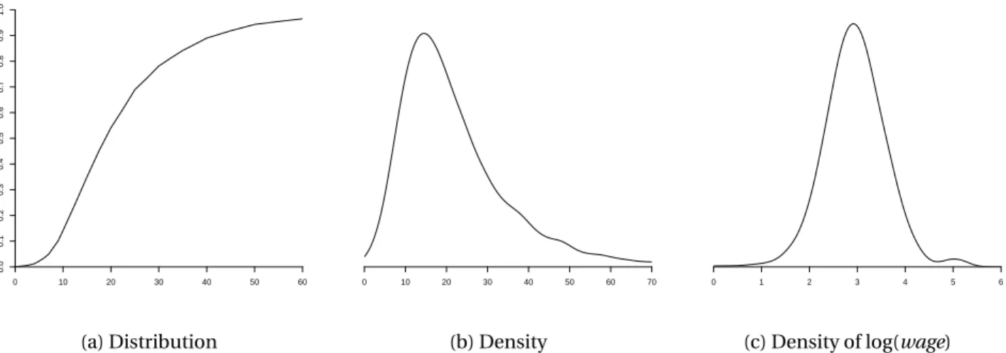
Suppose that we are interested in wage rates in the United States. Since wage rates vary across work- ers we cannot describe wage rates by a single number. Instead, we can describe wages using a probabil- ity distribution. Formally, we view the wage of an individual worker as a random variablewagewith the probability distribution
F(u)=P£
wage≤u¤ .
When we say that a person’s wage is random we mean that we do not know their wage before it is mea- sured, and we treat observed wage rates as realizations from the distributionF. Treating unobserved wages as random variables and observed wages as realizations is a powerful mathematical abstraction which allows us to use the tools of mathematical probability.
A useful thought experiment is to imagine dialing a telephone number selected at random, and then asking the person who responds to tell us their wage rate. (Assume for simplicity that all workers have equal access to telephones and that the person who answers your call will answer honestly.) In this thought experiment, the wage of the person you have called is a single draw from the distributionF of wages in the population. By making many such phone calls we can learn the full distribution.
When a distribution functionFis differentiable we define theprobability density function f(u)= d
d uF(u).
The density contains the same information as the distribution function, but the density is typically easier to visually interpret.
14
0 10 20 30 40 50 60
0.00.10.20.30.40.50.60.70.80.91.0
(a) Distribution
0 10 20 30 40 50 60 70
(b) Density
0 1 2 3 4 5 6
(c) Density of log(wage)
Figure 2.1: Wage Distribution and Density. All Full-time U.S. Workers
In Figure 2.1 we display estimates1 of the probability distribution function (panel (a)) and density function (panel (b)) of U.S. wage rates in 2009. We see that the density is peaked around $15, and most of the probability mass appears to lie between $10 and $40. These are ranges for typical wage rates in the U.S. population.
Important measures of central tendency are the median and the mean. Themedianmof a continu- ous distributionFis the unique solution to
F(m)=1 2.
The median U.S. wage is $19.23. The median is a robust2measure of central tendency, but it is tricky to use for many calculations as it is not a linear operator.
Themeanorexpectationof a random variableY with discrete support is µ=E[Y]=
X∞ j=1
τjP£ Y =τj¤
. For a continuous random variable with densityf