ExplicitRelationbetweenLow-DimensionalLLL-ReducedBasesandShortestVectors PAPER

PAPER Special Section on Discrete Mathematics and Its Applications

Explicit Relation between Low-Dimensional LLL-Reduced Bases and Shortest Vectors

Kotaro MATSUDA^†a), Atsushi TAKAYASU^†,††b),Nonmembers,andTsuyoshi TAKAGI^†c),Member

SUMMARY TheShortest Vector Problem(SVP) is one of the most im- portant lattice problems in computer science and cryptography. TheLLL lattice basis reduction algorithmruns in polynomial time and can compute anLLL-reduced basisthat provably contains an approximate solution to the SVP. On the other hand, the LLL algorithm in practice tends to solve low-dimensional exact SVPs with high probability, i.e.,>99.9%. Filling this theoretical-practical gap would lead to an understanding of the com- putational hardness of the SVP. In this paper, we try to fill the gap in 3,4 and 5 dimensions and obtain two results. First, we prove that given a 3,4 or 5-dimensional LLL-reduced basis, the shortest vector is one of the basis vectors or it is a limited integer linear combination of the basis vectors. In particular, we construct explicit representations of the shortest vector by using the LLL-reduced basis. Our analysis yields a necessary and sufficient condition for checking whether the output of the LLL algorithm contains the shortest vector or not. Second, we estimate the failure probability that a 3-dimensional random LLL-reduced basis does not contain the shortest vector. The upper bound seems rather tight by comparison with a Monte Carlo simulation.

key words: lattice, shortest vector problem, LLL algorithm, lattice-based cryptography

1. Introduction

1.1 Background

Public key cryptography is a fundamental technique for en- suring security in today’s information society. The RSA cryptosystem[37]and elliptic curve cryptosystem[19],[29]

are widely used, as exemplified by the SSL/TLS protocol.

Since the level of security relates to the hardness of the integer factorization and discrete logarithm problems that are believed to be computationally hard, the schemes are believed to be currently secure. However, due to Shor’s breakthrough work [42], these schemes can be broken in polynomial time by using a quantum algorithm. Therefore, constructing alternative cryptosystems that are secure in the post-quantum era has become the main stream of cryptog- raphy research. Lattice-based cryptography is one of the most promising candidates to resolve this issue. Its security relates to the hardness of the shortest vector problem (SVP).

Manuscript received October 1, 2018.

Manuscript revised January 22, 2019.

†The authors are with the Graduate School of Information Sci- ence and Technology, The University of Tokyo, Tokyo, 113-8654 Japan.

††The author is with National Institute of Advanced Industrial Science and Technology, Tokyo, 135-0064 Japan.

a) E-mail: [email protected] b) E-mail: [email protected] c) E-mail: [email protected]

DOI: 10.1587/transfun.E102.A.1091

Given a lattice basis, the goal of SVP is to find the shortest non-zero lattice vector. SVP is NP-hard under randomized reductions [1] and is believed to be computationally hard even against quantum adversaries.

Although several lattice-based schemes, e.g.,[15],[16], [36], have been proposed thus far, this does not suggest that they can be efficiently and securely used in practice. More concretely, we do not know the most suitable lattice dimen- sions for the best efficiency/security trade-off. To find them, we should examine the behavior of lattice basis reduction algorithmsthat are frequently used to estimate the hardness of SVPs. There are two types of SVP algorithm; one for solving exact SVPs, the other for solvingα-SVPs. Given a lattice basis, the goal of anα-SVP forα >1 is to find a lat- tice vector whose norm is at mostαtimes more than that of the shortest non-zero vector. In the context of the security of lattice-based cryptography, we want to estimate the running times ofα-SVPs for a small constantα, e.g.,α=1.05. In this paper, we focus on theLLL algorithm[23]. The LLL algorithm runs in polynomial time, but solves theα-SVP for only large α that is exponential in the lattice dimensions.

There are several (super-)exponential time algorithms for solving exact SVPs, e.g., enumeration[10],[20], sieve algo- rithms[2],[27], random sampling reductions[40], Voronoi cell computations[26], and so on, and all of them utilize the LLL algorithm as preprocessing. In addition, several reduc- tion algorithms e.g., BKZ reduction[38],[40], transference reduction [12], slide reduction [13], and so on, have been proposed for solving α-SVPs for smaller α than the LLL algorithm. All the algorithms are generalizations of the LLL algorithm and utilize it as a subroutine. Therefore, the LLL algorithm is a fundamental tool for solving (α-)SVPs and understanding the behavior of the LLL algorithm should be a crucial goal in the study of (α-)SVP algorithms.

The main stream of SVP is widely studied by many researchers especially in cryptography community. There are mainly two directions for studying the hardness of SVP, i.e., (1) practicalanalysis based on several heuristics, (2) theoretical analysis based on as strict discussion as possi- ble. The first approach (1) is the current main stream of this research area and has recently provided several fantas- tic results. Indeed, based on several heuristics such as the Gaussian heuristic, the geometric series assumption [39], and the randomness assumption[5],[11],[43], several faster SVP algorithms have been proposed. To solve the ex- act SVP, faster variants of enumeration [14], sieve algo- rithms [7],[9],[21],[22], [34], and random sampling re- Copyright © 2019 The Institute of Electronics, Information and Communication Engineers

ductions [5], [11], [24], [44] have been proposed. Sim- ilarly, faster variants of the LLL [30], [32], [35] and the BKZ[6],[8],[17],[28],[45]have been proposed.

What we study in this paper is differs from these works since we focus on the second approach (2). Since several substantial results have recently been proposed in the first approach (1), many readers tend to forget importance of the other approach (2). However, the second approach (2) is an arguably essential research topic for studying the hardness of SVP. In particular, we study theoretical behaviors of the LLL reduction in low dimensions. One may feel that LLL in low dimensions looks a weak target since we finally want to know practical behaviors of LLL in high dimensions or possibly BKZ-reduced bases. However, it is a much harder problem than one may expect. Indeed, as we will claim below there still exists fundamental problem regarding a behavior of LLL even in low dimensions. Furthermore, all papers which try to analyze high dimensional LLL-reduced bases or BKZ-reduced bases rely on experimental analysis or several heuristics. Therefore, low-dimensional LLL-reduced bases have to be a good target to put the research direction forward.

As we claimed above, the LLL algorithm has been proven to solve anα-SVP of exponentially large α. How- ever, it is actually much more effective in practice; it can solve exact SVPs with high probability in low dimensions.

Alsayigh et al.[4]found special classes of 3-dimensional lat- tice bases in which the LLL algorithm always/never solves the exact SVP. Moreover, low-dimensional SVPs have been studied by Semaév[41]and Nguyen and Stehlé[33]; they constructed efficient lattice reduction algorithms specific to 3 or 4 dimensions, but they did not analyze the relation to the LLL algorithm. Our motivation is rather similar to Al- sayigh et al.’s work[4]. Inspired by it, we decided to study the relationship between outputs of the LLL algorithm and shortest vectors in low dimensions.

1.2 Our Contributions

In this paper, we show an explicit relation between LLL- reduced bases and the shortest vectors in three, four and five dimensions. We prove that at least one of a few fixed linear integer combinations of the LLL-reduced basis vectors is the shortest non-zero vector in the lattice if the LLL-reduced basis does not contain the shortest non-zero vector in three, four and five dimensions. From this, we obtain a necessary and sufficient condition that an LLL-reduced basis does not contain the shortest vector. For example, if a 3-dimensional LLL-reduced basis(b₁,b₂,b₃)does not contain the shortest non-zero vector in the latticeL(b₁,b₂,b₃), then eitherb₂±b₃ orb₁±b₂±b₃is the shortest non-zero vector in the lattice L(b₁,b₂,b₃). Thus, we can easily find one of the shortest non-zero vectors in the lattice by changing the LLL algorithm slightly. Moreover, by using this condition, we estimate the failure probability that a random LLL-reduced basis does not contain the shortest vector in three dimensions. To be more precise, we consider 6-dimensional space where each point is corresponded to a 3-dimensional basis, and then we

estimate the ratio of the volume of the region corresponded to LLL-reduced bases not containing the shortest vector over that of the region corresponded to LLL-reduced bases. We calculate its upper bound by numerical integration. We also show that the upper bound we obtain is about twice the value obtained in a Monte Carlo simulation.

1.3 Organization

In Sect. 2, we recall the basic notions of lattices, SVP, and LLL algorithm. In Sect. 3, we show the explicit relation between LLL-reduced bases and the shortest vectors in three, four and five dimensions. In Sect. 4, we estimate the failure probability that a 3-dimensional random LLL-reduced basis does not contain the shortest vector. In addition, we compare the upper bound with the value obtained by the Monte Carlo method.

2. Preliminaries

In this section, we recall the basic definitions of lattices and the (α-)shortest vector problem (SVP). Then, we explain the LLL algorithm and its behavior in low dimensions.

2.1 Notation

LetRandZdenote a set of real numbers and integers, re- spectively. Let a lowercase bold letter b denote a vector whose transpose is denoted by b^>. The Euclidean norm of a vector b is denoted by kbk. The inner product ofb₁ and b₂ is denoted by hb₁,b₂i. Let (b₁, ...,bn) be a set of linearly independent vectors. The Gram-Schmidt orthog- onal basis (b₁^∗, ...,b^∗_n) is defined as follows: b₁^∗ = b₁ and b^∗_i = b_i −Pi−1

j=1µ_{i j}b^∗_j for 2 ≤ i ≤ n, where µ_{i j} = ^hb_kb^i,b∗∗ji

jk2

are called Gram-Schmidt orthogonal coefficients. We will sometimes writeµ_{i j}as µ_i,jin this paper.

2.2 Lattices

A lattice is an additive discrete subgroup of R^m. Let (b₁, ...,bn) ∈ R^n×m be a set of linearly independent vec- tors. A lattice spanned by a basis (b₁, ...,b_n)is defined as L(b₁, ...,bn)={Pn

i=1x_ibi|x_i ∈Z}. For simplicity through- out the paper, we will study only full-rank lattices, i.e., n=m.

Letλ₁(L(b₁, ...,bn))denote the Euclidean norm of the shortest non-zero vector inL(b₁, ...,bn). We define theSVP as follows.

Definition 1(SVP): Given a basis(b₁, ...,bn), the goal of the SVP is to find a vectorb⁰in a lattice L(b₁, ...,bn)such thatkb⁰k=λ₁(L(b₁, ...,bn))holds.

Ajtai proved that the SVP is NP-hard under randomized re- duction[1].

There is also an approximate version parameterized by α >1.

Definition 2(α-SVP): Given a basis(b₁, ...,bn)and a real numberα >1, the goal of theα-SVP is to find a vectorb⁰in a lattice L(b₁, ...,bn) such thatkb⁰k ≤ αλ₁(L(b₁, ...,bn)) holds.

Khot proved that the α-SVP is NP-hard if α is a constant under randomized reductions[18].

2.3 LLL Algorithm

Here, we recall theLLL algorithm, which is a fundamental tool for solving the (α-)SVP.

Lattices do not have unique bases. There exist infinitely many bases for the same lattice under unimodular transfor- mations. Given a lattice basis, the LLL algorithm outputs an LLL-reduced basisdefined as follows.

Definition 3(LLL-reduced Basis): Letδbe a real number withδ∈(1/4,1]. If a basis(b₁, ...,bn) ∈R^n×nsatisfies the following two conditions, it is called an LLL-reduced basis with a Lovász factorδ:

• Size reduction: |µi j| ≤1/2 holds for alli,jwith 1≤j <i≤n,

• Lovász condition: kb^∗_i +µ_i,i−1b^∗_i−1k²≥δkb_i−^∗₁k²hold for alliwith 2≤i ≤n.

The LLL algorithm runs in O(n⁶log³(max(kb₁k, ...,kb_nk))) time for δ < 1 (it has been proven for δ = 1 in a fixed number of dimensions that it runs in polynomial time of input size [3]) and outputs LLL-reduced bases. In using the LLL algorithm,δis usually strictly smaller than 1. In this paper, we also consider the case of δ = 1, which is called “ideal” or “optimal”. The first vectorb₁of an LLL- reduced basis is a solution of anα-SVP forα= ₄

4δ−1

ⁿ⁻₂¹ , i.e., kb₁k ≤ ₄

4δ−1

ⁿ⁻¹₂

λ₁(L(B)) holds. Hence, a smaller Lovász factor enables us to solveα-SVP for a largerα. In the special casen = 2, LLL for δ = 1 is the same as the Lagrange-Gauss reduction algorithm (see e.g.[31]). Hence, LLL runs in polynomial time and outputs the shortest vectors.

It is well known that LLL outputs much shorter vectors in practice. Specifically, in three to ten dimensions, it can solve an SVP with a probability of more than 99.9% by taking a factorδclose to 1 (δ >0.999)[4].

In this paper, we say that a basis(b₁, ..,b_n)does not con- tain the shortest non-zero vector ifkbik,λ₁(L(b₁, ...,bn)) holds for 1≤i ≤n. In addition, we say the failure condition is when an LLL-reduced basis does not contain the shortest non-zero vector.

3. Failure Condition of LLL-Reduced Bases

Here, we discuss the necessary and sufficient condition that an LLL-reduced basis does not contain the shortest vector.

Indeed, we show how the shortest vector can be represented by an integer linear combination of an LLL-reduced basis vectors.

3.1 Case of Three Dimensions andδ=1

First, we discuss the case ofn=3 dimensions and a Lovász factor δ=1 in Definition 3. In this case, we can prove the following theorem.

Theorem 1: Suppose a 3-dimensional LLL-reduced ba- sis (b₁,b₂,b₃) for a Lovász factor δ = 1 does not con- tain the shortest non-zero vector in the lattice L(b₁,b₂,b₃). If b⁰ = P₃

i=1x_ibi for some integers x₁,x₂,x₃ is the shortest non-zero vector in the lattice L(b₁,b₂,b₃), then (|x₁|,|x₂|,|x₃|) = (1,1,1) or (0,1,1) holds. In addi- tion, there exist LLL-reduced bases (b₁,b₂,b₃) such that b⁰=P₃

i=1x_ibiis the shortest vector inL(b₁,b₂,b₃)for each (|x₁|,|x₂|,|x₃|)=(1,1,1)or(0,1,1).

Proof 1: The Gram-Schmidt orthogonal basis (b₁^∗,b^∗₂,b^∗₃) satisfiesb₁=b^∗₁,b₂ =µ₂₁b^∗₁+b^∗₂,b₃=µ₃₁b₁^∗+µ₃₂b₂^∗+b^∗₃. Hence,(b₁,b₂,b₃)can be represented as linear combinations of orthogonal basis vectors _b∗

kb1^∗₁k,_kb^b∗2∗ 2k,_kb^b∗3∗

3k

as follows:

* . ,

b₁^>

b₂^>

b₃^>

+ / -

=* . ,

kb^∗₁k 0 0

µ₂₁kb₁^∗k kb₂^∗k 0 µ₃₁kb₁^∗k µ₃₂kb^∗₂k kb^∗₃k

+ / -

* . . . ,

1 kb^∗₁kb^∗₁^>

1 kb^∗₂kb^∗₂^>

1 kb^∗₃kb^∗₃^>

+ / / / - .

(1) Since (b₁,b₂,b₃) is LLL-reduced, we have the following inequalities:

kb₂^∗k² ≥(1−µ²₂₁)kb₁^∗k² ≥ 3

4kb^∗₁k², (2) kb₃^∗k² ≥(1−µ²₃₂)kb₂^∗k² ≥ 3

4kb^∗₂k²≥ 9

16kb^∗₁k². (3) Ifx₃satisfies|x₃| ≥2, the vectorb⁰=P3

i=1xibi fulfills the following inequality:

kb⁰k² ≥(2kb^∗₃k)²=4kb^∗₃k² ≥9

4kb^∗₁k² >kb₁k². (4) Therefore, if b⁰ is the shortest non-zero vector, |x₃| ≤ 1 holds.

Ifx₃=0 holds,b⁰is inL(b₁,b₂). The 2-dimensional LLL algorithm forδ=1 is equivalent to the Lagrange-Gauss reduction algorithm. Therefore, kb₁k = λ₁(L(b₁,b₂)) or kb₂k = λ₁(L(b₁,b₂)). Consequently, if the LLL-reduced basis(b₁,b₂,b₃)does not contain the shortest non-zero vec- tor andb⁰is the shortest vector,|x₃|=1.

Next, ifx₂satisfies|x₂| ≥2,

kb⁰k² ≥ |x₃|²kb^∗₃k²+(x₃µ₃₂+x₂)²kb^∗₂k²

≥ 9

4kb₂^∗k² ≥ 27

16kb₁^∗k² >kb₁k²

holds in accordance with the size reduction, equations (1), (3) and|x₃|=1. This contradicts the shortest property ofb⁰ and thus|x₂| ≤1 holds.

Finally we prove|x₁| ≤ 1. Fromb⁰ =P₃

i=1x_ibi, we have the equality kb⁰k² = (x₁ +µ₂₁x₂+µ₃₁x₃)²kb^∗₁k² + (x₂+µ₃₂x₃)²kb^∗₂k²+x²₃kb^∗₃k². From|x₂| ≤1,|x₃| ≤1 and the size reduction,|µ₂₁x₂+µ₃₁x₃| ≤1 holds. Therefore, if b⁰is the shortest non-zero vector,|x₁| ≤1.

Moreover, if (|x₁|,|x₂|,|x₃|) = (1,0,1), kb⁰k ≥ kb₃k holds by the size reduction. From the above, if b⁰ = P₃

i=1x_ib_iis the shortest vector,(|x₁|,|x₂|,|x₃|)=(1,1,1)or (0,1,1)holds. This means we find LLL-reduced bases that do not contain the shortest vector for each occasion (this is

shown in Appendix A).

This theorem leads to the following corollary.

Corollary 1: For a Lovász factorδ=1, the following is a necessary and sufficient condition that an LLL-reduced basis (b₁,b₂,b₃)does not contain the shortest vector: One of the vectors b₂ ±b₃ or b₁ ±b₂±b₃ (the signs are exclusively alternating) is shorter thanb₁,b₂,andb₃.

From this corollary, we can obtain one of the shortest non-zero vectors using the output of the LLL algorithm and comparing the norm ofb₁,b₂,b₃ with those of linear com- binationsb₂±b₃andb₁±b₂±b₃. We note that the result is derived for analyzingtheoreticalbehaviors of LLL-reduced bases. Specifically, even when we obtain analogous results for high dimensions, they do not seem useful to speed-up practical enumeration. In particular, although we do not use any heuristics during the analysis, practical enumeration based on several heuristics has to be faster than the above analysis.

The representation of the shortest vectors by limited number of integer linear combinations may look similar to natural number representation/tag in the context of enumer- ation and random sampling reduction[5],[11],[24],[44].

However, unfortunately we cannot find close relation with these notions. Furthermore, unlike ours the researchs[5], [11],[24],[44]are heavily based on several heuristics, e.g., randomness assumption[43].

3.2 Case of Three Dimensions andδ <1

Next, we extend Theorem 1 to the case of a Lovász factor δ < 1. Note that the LLL algorithm often uses ³₄ ≤δ, but we prove the following theorem for the case of ₁₂⁷ ≤δ≤1.

Theorem 2: Theorem 1 holds for a Lovász factor₁₂⁷ ≤δ≤ 1.

Proof 2: From the size reduction, the Lovász condition and

127 ≤δ≤1, we have kb^∗₂k² ≥ δ−1

4

!

kb^∗₁k² ≥ 1

3kb₁^∗k²and kb^∗₃k² ≥ δ−1

4

!

kb^∗₂k² ≥ 1 3kb₂^∗k².

Supposex₃ ≥2, then we obtain the following inequality:

kb⁰k² ≥4kb^∗₃k² ≥ kb₃^∗k²+kb₂^∗k²

≥ kb^∗₃k²+1

4kb₂^∗k²+1

4kb₁^∗k² ≥ kb₃k². This implies|x₃| ≤1.

Now, let us provex₃,0. kb⁰k² ≥4kb₂^∗k² ≥ ⁴₃kb^∗₁k²>

kb₁k² holds for x₃ = 0 and |x₂| ≥ 2. kb⁰k² ≥ kb₂^∗k² + (x₁+µ₁₂)²kb^∗₁k² ≥ kb₂k² holds for x₃ = 0 and|x₂| =1.

kb⁰k ≥ kb₁kholds for x₃ =0 andx₂ =0. This contradicts the shortest property ofb⁰. Thereforex₃,0,i.e.,|x₃|=1.

If|x₂| ≥2, kb⁰k² ≥ 9

4kb₂^∗k²+kb₃^∗k²

≥ 2

3kb₁^∗k²+1

4kb₂^∗k²+kb₃^∗k² >kb₃k²

holds by the size reduction and kb^∗₂k ≥ ¹₃kb^∗₁k. Therefore

|x₂| ≤1 holds. A discussion similar to the proof in the case ofδ=1 leads to|x₁| ≤1.

Thus, Theorem 2 is proved.

A corollary similar to Corollary 1 holds for ₁₂⁷ ≤δ≤1.

3.3 Case of Four and Five Dimensions andδ=1

An ideal goal of our approach has to be an extension for the asymptotic case. However, to avoid using any heuristics, the computations during the analyses take huge amount of times. For example, we list all the possible linear combi- nations to find the shortest vector and the listing is at least harder than solving SVP. Therefore, providing the analogous analysis in high dimensions without any heuristics has to be an intractable problem. In this paper, to observe analogous behaviors for higher dimensions, we prove theorems in the case of n =4 or 5 dimensions and a Lovász factorδ =1.

The proofs are similar to that of Theorem 1 (Summaries are in Appendix B).

Theorem 3: Suppose a 4-dimensional LLL-reduced ba- sis (b₁,b₂,b₃,b₄) for a Lovász factor δ = 1 does not contain the shortest non-zero vector in the lattice L(b₁,b₂,b₃,b₄). Then one of the vectorsP₄

i=1x_ibisatisfy- ing (|x₁|,|x₂|,|x₃|,|x₄|) = (0,1,1,0),(1,1,1,0),(0,0,1,1), (1,0,1,1),(0,1,0,1),(1,1,0,1),(0,1,1,1)or(1,1,1,1)is the shortest vector in L(b₁,b₂,b₃,b₄). In addition, there exist LLL-reduced bases(b₁,b₂,b₃,b₄)such thatb⁰=P₄

i=1x_ibi

for each (|x₁|,|x₂|,|x₃|,|x₄|) of the above equation is the shortest vector inL(b₁,b₂,b₃,b₄).

Theorem 4: Suppose a 5-dimensional LLL-reduced ba- sis (b₁,b₂,b₃,b₄,b₅) for a Lovász factor δ = 1 does not contain the shortest non-zero vector in the lattice L(b₁,b₂,b₃,b₄,b₅). Then one of the vec- tors P₅

i=1x_ibi satisfying (|x₁|,|x₂|,|x₃|,|x₄|,|x₅|) = (0,1,1,0,0),(1,1,1,0,0),(0,0,1,1,0),(1,0,1,1,0),

(0,1,0,1,0),(1,1,0,1,0),(0,1,1,1,0),(1,1,1,1,0), (0,1,0,0,1),(0,0,1,0,1),(0,0,0,1,1),(1,1,0,0,1), (1,0,1,0,1),(1,0,0,1,1),(0,1,1,0,1),(0,1,0,1,1),

(0,0,1,1,1),(1,1,1,0,1),(1,1,0,1,1),(1,0,1,1,1), (0,1,1,1,1),(1,1,1,1,1),(2,1,1,1,1),(0,2,1,1,1),

(1,2,1,1,1) or (2,2,1,1,1) is the shortest vector in L(b₁,b₂,b₃,b₄,b₅). In addition, there exist LLL-reduced bases(b₁,b₂,b₃,b₄,b₅)for each(|x₁|,|x₂|,|x₃|,|x₄|,|x₅|)of the above equation such thatb⁰=P₅

i=1x_ibi is the shortest vector inL(b₁,b₂,b₃,b₄,b₅).

From these theorems, we can easily find one of the shortest non-zero vectors in a four or five-dimensional lat- tice by changing the LLL algorithm slightly. Namely, if a 4 or 5-dimensional LLL-reduced basis does not contain the shortest non-zero vector in the lattice, then one of the vec- tors appearing in Theorems 3 and 4 is the shortest non-zero vector.

4. Estimating the Failure Probability in Three Dimen- sions

In this section, we estimate the failure probability that a 3-dimensional random LLL-reduced basis does not con- tain the shortest vector. We consider six-dimensional space parameterized by six variables (kb₁^∗k,kb₂^∗k,kb^∗₃k, µ₂₁kb^∗₁k, µ₃₁kb^∗₁k, µ₃₂kb^∗₂k). In the space, each point is correspond one-to-one with a basis(b₁,b₂,b₃)since(b₁,b₂,b₃)is de- termined by (kb₁^∗k,kb₂^∗k,kb^∗₃k, µ₂₁kb^∗₁k, µ₃₁kb^∗₁k, µ₃₂kb^∗₂k). We estimate the ratio of the volume of the region corre- sponded to LLL-reduced bases not containing the shortest vector over that of the region corresponded to LLL-reduced bases. We obtain its upper bound by numerical integration and compare it with the value obtained by the Monte Carlo method.

4.1 Projection Region

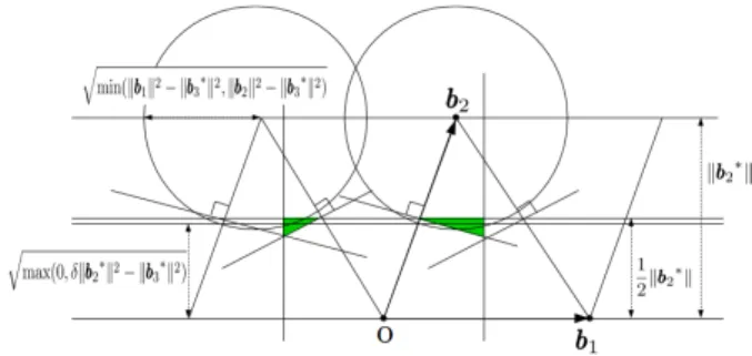
Here, in order to estimate the failure probability by inte- gration, we first describe the condition for an LLL-reduced basis(b₁,b₂,b₃)by projectingb₃on the planeHspanned by (b₁,b₂). For a fixed(b₁,b₂)satisfyingkb₂k²≥δkb₁k², the blue rectangular region in Fig. 1 shows the condition for the possible projection ofb₃onHsuch that(b₁,b₂,b₃)is LLL- reduced. For simplicity we show the region that satisfies µ₂₁ ≥0 andµ₃₂ ≥0. The width of the rectangle is deter- mined by the size reduction of |µ₃₁| ≤ ¹₂ appearing in the LLL-reduced basis. The heights of the upper and lower parts of the rectangle are decided by the size reduction|µ₃₂| ≤ ¹

2, and the Lovász condition,kb^∗₃k² +µ²₃₂kb^∗₂k² ≥ δkb₂^∗k, re- spectively.

Next, we explain the condition for an LLL-reduced basis (b₁,b₂,b₃)not containing the shortest vector. By Theorem 2, if a 3-dimensional LLL-reduced basis does not contain the shortest vector, b₂±b₃ or b₁ ±b₂±b₃ (the signs are exclusively alternating) is the shortest vector. Therefore, kb₂±b₃k < min(kb₁k,kb₂k,kb₃k) or kb₁ ±b₂ ±b₃k <

min(kb₁k,kb₂k,kb₃k) holds in this case. Thus, for fixed b₁,b₂ andb₃^∗, the region of the projection ofb₃ ontoHis the red region in Fig. 2 if the LLL-reduced basis(b₁,b₂,b₃)

Fig. 1 Region of the projection ofb₃onto a planeH=span(b₁,b₂) (blue region : (b₁,b₂,b₃)is an LLL-reduced basis).

Fig. 2 Region of the projection ofb₃onto a planeH=span(b1,b₂) (red region :(b₁,b₂,b₃)is an LLL-reduced basis not containing the short- est vector).

Fig. 3 Region of the projection ofb₃onto a planeH=span(b1,b₂).

does not contain the shortest vector.

4.2 Upper Bound of the Failure Probability in Three Di- mensions

In three dimensions, we estimate the failure probability that a 3-dimensional random LLL-reduced basis does not contain the shortest vector. This failure probability can be calculated as the ratio of the volume of the red region in Fig. 2 over that of the blue region in Fig. 1. However, the calculation of the volume of the red region is relatively hard, and thus we eval- uate the volume of the green region in Fig. 3, which contains the red region. To calculate the volumes of the blue and green regions, we use numerical integration over six variables (kb₁^∗k,kb^∗₂k,kb^∗₃k, µ₂₁kb^∗₁k, µ₃₁kb₁^∗k, µ₃₂kb₂^∗k). In particu- lar, the calculation can be used to estimate the volume of the hypersurface in six-dimensional space parameterized by the above variables.

Here, we prove the following theorem for estimating the upper bound of the failure probability.

Theorem 5: Let S be six dimensional space (kb^∗₁k,kb^∗₂k, kb^∗₃k, µ₂₁kb^∗₁k, µ₃₁kb₁^∗k, µ₃₂kb₂^∗k). LetD⊂Sbe the region corresponded LLL-reduced bases(b₁,b₂,b₃). LetE ⊂ S be the region corresponded LLL-reduced bases(b₁,b₂,b₃) not containing the shortest vector in the latticeL(b₁,b₂,b₃). LetPbe the failure probability calculated as the ratio of the volume ofEover that ofD. ThenP<2.94×10⁻⁴holds by taking Lovász factorδ=1.

If we fixkb^∗₁k,kb^∗₂k,kb₃^∗k,andµ₂₁kb₁^∗k, the regionDandE is shown as the blue region in Fig. 1 and the red one in Fig. 2, respectively. Therefore, we try to integrate their volume.

Proof 3: If the value kb^∗₁k kb^∗₂k kb₃^∗k is fixed, the ratio of volume of the regionEover that of the regionDis constant independently of the value kb₁^∗k kb^∗₂k kb^∗₃k. Therefore, we estimate P under the scaling kb^∗₁k kb₂^∗k kb₃^∗k = 1. Let V be the volume of the region D under kb^∗₁k kb^∗₂k kb₃^∗k = 1.

Since the green region in Fig. 3 contains the red region in Fig. 2 corresponding toE in Theorem 5, the failure proba- bilityPis less thanU/VwhereUis the volume of the green region in Fig. 3 underkb^∗₁k kb₂^∗k kb^∗₃k =1. We can calcu- lateU andV by using numerical integration over six vari- ables (kb^∗₁k,kb^∗₂k,kb^∗₃k, µ₂₁kb₁^∗k, µ₃₁kb₁^∗k, µ₃₂kb^∗₂k) under the scalingkb^∗₁k kb^∗₂k kb₃^∗k=1.

First, we discuss the possible ranges of the six variables (kb^∗₁k,kb^∗₂k,kb₃^∗k, µ₂₁kb₁^∗k, µ₃₁kb₁^∗k, µ₃₂kb^∗₂k). We may as- sumeµ₂₁ ≥ 0 by symmetry of the conditions for an LLL- reduced basis. From the size reduction and the Lovász con- dition of the LLL-reduced basis(b₁,b₂,b₃), we have

0≤ kb₁^∗k ≤ kb₂^∗k qδ−¹₄

, 0≤ kb₂^∗k ≤ kb₃^∗k

qδ−¹₄

= 1

qδ−¹₄kb₁^∗k kb^∗₂k .

Therefore,

0≤ kb^∗₁k ≤min* . . ,

kb₂^∗k qδ−¹₄

, 1

qδ−¹₄kb^∗₂k² + / / -

(5)

holds. In addition, from the size reduction and the Lovász condition, 0≤ µ₂₁kb^∗₁k ≤ ¹₂kb^∗₁kandµ²₂₁kb^∗₁k²+kb₂^∗k² ≤ δkb^∗₁k². Thus,

qmax(0, δkb₁^∗k²− kb₂^∗k²) ≤µ₂₁kb^∗₁k ≤ kb^∗₁k 2 . (6) Therefore, the area of the blue domain in Fig. 1 is kb^∗₁k(^kb

∗1k

2 −

qmax(0, δkb^∗₁k²− kb^∗₂k²)).

From the above discussion,V can be calculated by in- tegration, as follows:

V=Z ∞ 0

Z ^min*

,

√y δ−1

4 ,√ ¹

δ−1 4y2+

-

0 x x

2 −

qmax(0, δx²−y²)

!

·

* . , y 2 −

vt max*

,

0, δ y²− 1 xy

!2

+ - + / -

px⁴y⁴+x²+y² x²y² dx

dy,

where x = kb^∗₁k, y = kb^∗₂k. (Note that

√

x⁴y⁴+x²+y² x²y² is the Jacobian underkb₁^∗k kb^∗₂k kb^∗₃k=1.)

Next, we evaluate the upper bound ofU. Ifb₁,b₂andb^∗₃ are fixed, the area of the green region in Fig. 2 is ^kb₄^∗1k·^µ12kb

∗1k kb₂^∗k · _kb∗

1k 2 −^µ12kb

∗1k 2

. When the LLL-reduced basis(b₁,b₂,b₃) does not contain the shortest vector, λ₁(L(b₁,b₂,b₃))² ≥ kb₃^∗k² + ¹₄kb₂^∗k² holds by Theorem 1. Therefore, from kb₁^∗k kb₂^∗k kb^∗₃k=1 andkb₁k ≥λ₁(L(b₁,b₂,b₃)), we have

kb₁k² ≥ 1 kb^∗₁k kb^∗₂k

!2

+1 4kb^∗₂k². This inequality implies

kb₁^∗k ≥ vu ut

kb₂^∗k³+q

kb^∗₂k⁶+64

8kb^∗₂k . (7)

From (5) and (7), ifkb₂^∗k ≤1 holds, _(δ−1

4)² 1−¹₄(δ−¹₄)

¹₆

≤ kb^∗₂k ≤ 1, otherwise 1≤ kb^∗₂k ≤

1 δ(δ−¹₄)

¹₆ holds.

From the above discussion,U can be estimated as fol- lows:

U=Z ₁

(δ−1 4)2 1−1

4(δ−1 4)

!¹₆

Z √^y

δ−1 4 ry3+√

y6+64 8y

x 4*

, Z ^x₂

0

t y

x 2 − t

2 dt+

- px⁴y⁴+x²+y²

x²y² dx

! dy

+ Z ¹

δ(δ−1 4)

!¹₆ 1

Z √ ¹

δ−1 4y2 ry3+√

y6+64 8y

x 4*

, Z ^x₂

0

t y

x 2 − t

2 dt+

- px⁴y⁴+x²+y²

x²y² dx! dy

=Z 1 (δ−1

4)2 1−1

4(δ−1 4)

!¹₆

* . . , Z

√y δ−1

4 ry3+√

y6+64 8y

x³p

x⁴y⁴+x²+y² 96y³ dx+

/ / -

dy

+ Z ¹

δ(δ−1 4)

!1 6 1

* . . ,

Z √ ¹

δ−1 4y2 ry3+√

y6+64 8y

x³p

x⁴y⁴+x²+y² 96y³ dx+

/ / -

dy, where x = kb^∗₁k, y = kb₂^∗k andt = µ₂₁kb₁^∗k. By taking δ=1, we can calculateVandUby numerical integration to beV ;0.439 andU;0.000129. Therefore, the probability

Psatisfies P<U

V ; 0.000129

0.439 ;2.94×10⁻⁴.

According to this proof, we have theoretically obtained that a random LLL-reduced basis contains the shortest vector with high probability,i.e. more than 99.9%, by taking a factorδ close to 1.

4.3 Monte Carlo Simulation

We estimate the failure probabilityPin Theorem 5 by using a Monte Carlo simulation. Under kb₁^∗k kb^∗₂k kb^∗₃k = 1, the LLL-reduced basis (b₁,b₂,b₃)is represented as follows:

b₁ =* . ,

kb^∗₁k 00

+ / -

, b₂=* . ,

µ₂₁kb^∗₁k kb^∗₂k

0 + / -

, b₃ =* . . ,

µ₃₁kb^∗₁k µ₃₂kb^∗₂k

kb₁^∗k k1b^∗₂k

+ / / - . Since it is too difficult to sample an LLL-reduced ba- sis uniformly at random, we use the sampling which is not uniformly at random in reality. Therefore, we merely cal- culate the approximate value of the failure probability by Monte Carlo simulation. In our experiment, in order to sample LLL-reduced bases as uniformly random as possible under kb^∗₁k kb^∗₂k kb^∗₃k = 1, we first sample lattice bases as uniformly random as possible so that the sampling domain contains almost all LLL-reduced bases. Then we check whether the sampled bases are LLL-reduced or not. Finally we check whether the sampled LLL-reduced bases contain the shortest vector or not. For the purpose, we first sample kb^∗₁kin a range [0.0,1.3], kb₂^∗kin [0.0,10.0], µ₂₁kb^∗₁kand µ₃₁kb^∗₁kin [−0.65,0.65], andµ₃₂kb^∗₂kin [−5.0,5.0] by using Mersenne twister[25]. We set the upper bounds ofµ₂₁kb^∗₁k, µ₃₁kb^∗₁k, andµ₃₂kb^∗₂kdue to the size reduction|µ₂₁| ≤ ¹₂,

|µ₃₁| ≤ ¹₂, and|µ₃₂| ≤ ¹₂. The range ofkb^∗₁kis adequate becausekb₁^∗k ≤ √²

3 <1.3 if(b₁,b₂,b₃)is LLL-reduced and kb^∗₁k kb^∗₂k kb₃^∗k=1. Althoughkb^∗₂kis not bounded above by a constant which is independent ofkb₁^∗k, we need to bound the range of kb^∗₂k to demonstrate our experiment. To be precise, we also tried the experiment with a larger bound ofkb^∗₂k; however, in this case sampled lattice bases are not LLL-reduced with high probability. In our experiment with the upper boundkb^∗₂k ≤10.0, we sampled 76,429,270,520 bases and there were 60,000,000 LLL-reduced bases, of which 8,736 contained no shortest vector. This approximate failure probability is _60,000,000^8,736 '1.46×10⁻⁴. In addition, in the case the upper bound of kb₂^∗k ≤ 40.0, we sampled 12,236,665,172 bases and there were 600,000 LLL-reduced bases, of which 77 contained no shortest vector. This ap- proximate failure probability is _600,000⁷⁷ '1.28×10⁻⁴. The approximate failure probabilities in both experiments are al- most the same. Therefore, we consider 10.0 is sufficient for the upper bound ofkb^∗₂k and we used 10.0 as the up- per bound. From above, the approximate value of P is

8,736

60,000,000 '1.46×10⁻⁴. The upper bound of P in Theo- rem 5 is of the same magnitude as the above value. More precisely, the upper bound of the failure probability in Theo- rem 5 is about twice as large as the value obtained by Monte Carlo simulation.

5. Conclusion

We studied the explicit relation between LLL-reduced bases and the shortest vectors in three, four and five dimensions.

We presented a necessary and sufficient condition that the output of the LLL algorithm does not contain the shortest vector in three dimensions for ₁₂⁷ ≤δ ≤1. From this con- dition, we can construct the reduction algorithm for solving SVP with probability 1 by slightly modifying the LLL al- gorithm (by checking a few integer linear combinations of the output). Moreover, we analyzed the probability that a basis does not contain the shortest vector in three dimen- sions. We proved the upper bound of the failure probability is 2.94×10⁻⁴ forδ =1 by evaluating the volume of space that satisfies the above necessary and sufficient conditions.

In the case of four and five dimensions, we presented the necessary and sufficient conditions forδ =1 similar to the one in three dimensions.

It is interesting open problem that investigate the ex- plicit relation of LLL-reduced bases in more than five di- mensions and possibly an asymptotic case. As we claimed in Section 3.3, the extension in an asymptotic case should rely on some heuristic assumptions. If we obtain such ex- tensions under mild assumptions, the result should be inter- esting. Furthermore, analogous analysis for BKZ-reduced bases is also an interesting open problem.

Acknowledgements

We would like to thank anonymous reviewers of this journal for their insightful comments to improve the paper. This work was supported by JST CREST Grant Number JP- MJCR14D6, Japan.

References

[1] M. Ajtai, “The shortest vector problem inL₂isNP-hard for random- ized reductions (extended abstract),” Proc. STOC 1998, J.S. Vitter, ed., pp.10–19, ACM, 1998.

[2] M. Ajtai, R. Kumar, and D. Sivakumar, “A sieve algorithm for the shortest lattice vector problem,” Proc. STOC 2001, J.S. Vitter, P.G.

Spirakis, and M. Yannakakis, eds., pp.601–610, ACM, 2001.

[3] A. Akhavi, “The optimal LLL algorithm is still polynomial in fixed dimension,” Theor. Comput. Sci., vol.297, no.1-3, pp.3–23, 2003.

[4] S. Alsayigh, J. Ding, T. Takagi, and Y. Wang, “The beauty and the beasts - The hard cases in LLL reduction,” Proc. IWSEC 2017, S.

Obana and K. Chida, eds., LNCS 10418, pp.19–35, Springer, 2017.

[5] Y. Aono and P.Q. Nguyen, “Random sampling revisited: Lattice enumeration with discrete pruning,” Proc. EUROCRYPT 2017, J.

Coron and J.B. Nielsen, eds., LNCS 10211, pp.65–102, 2017.

[6] Y. Aono, Y. Wang, T. Hayashi, and T. Takagi, “Improved progressive BKZ algorithms and their precise cost estimation by sharp simulator,”

Proc. EUROCRYPT 2016, M. Fischlin and J. Coron, eds., LNCS 9665, pp.789–819, Springer, 2016.