A Unifying Framework of Combinatorial Optimization Algorithms; Tree Programming and Its Validity

Journal of the Operations Research Society of Japan

Vo!. 24,No.l, March 1981

A UNIFYING

OPTIMI ZA TION

FRAMEWORK OF COMBINATORIAL

ALGORITHMS; TREE PROGRAMMING

AND ITS VALIDITY

Yasuki Sekiguchi

Hokkaido University

(Received May 12, 1980; Revised August 20,1980)

Abstract A unifying framework, named tree programming, for solution algorithms of combinatorial optimization problems, such as branch-and-bound algorithms, dynamic programming, backtrack programming, additive implicit enumeration and cuttmg plane methods, is proposed. Constituents of tree programming are a selection rule, a branching rule, an upper bounding function, an elimination rule and a terminating condition. The essential difference from conventional models of such algorithms is in the abstract definition of elimination rules. The validity of tree program-ming, fmiteness and correctness, is examined. It is shown that finiteness is mainly dominated by the selection rule and the elimination rule, and that correctness by the terminating condition. As examples of tree programming, algorithms cited above are reformulated along the proposed framework.

1_

Introduction

Combinatorial or discrete opt imizat Lon problems have been one of the :nain concerns in the past two decades or more in mathematical programming resea~ch. Unfortunately, there has been no unified theory of optimal solutions but many solution algorithms have been proposed. It seems to be difficult to have a universal solution algorithm for a varie-~y of combinatorial problems. Indeed, most of the proposed algorithms are effieient only for certain types of prob-lems and moreover for certain types of nlunerical data on certain types of problems (cf. pp .16-17 in (19)) _ Recently" several researches on the complexity of computations have strongly suggested that the situation above comes from the nature of combinatorial problems and is not a temporary matter[ll). In ad-dition, experience tells us that the solution algorithms for slightly different problems are usually very different. For example, an algorithm for an asym·-metric travelling salesman problem is not effective for the symasym·-metric one.

All these seem to imply that under nany practical situations they must develop their own algorithms to solve their problems efficiently. Standing on

67

68 Y. Sekiguchi

this point, possibilities of a unified theory on the solution algorithms, especially, on how to make an algorithm efficient, should be explored. This paper aims to give a basis of such research.

There are several general approaches to construct algorithms, e.g. branch-and-bound methods[l,3,9,15,17,21], dynamic programming[7,18], backtrack pro-gramming[6,23,25], cutting plane methods[5,8], etc. and many particular algo-rithms. But, each approach utilizes different mechanisms to make it effective. It is natural to try to compose different mechanisms into a single algorithm[ 9,10,13,14,18,21]. In doing this, it will be convenient to have a unified model of these algorithmE.

If the scope is restricted within integer programming problems, most of the proposed algorithms axe unified in the framework of Geoffrion and Marsten

[5]. If restricted within the algorithms of branch-and-bound and dynamic pro-gramming types, they are unified in the framework of Kohler and Steiglitz[13] or Ibaraki [10]. Tree programming, the proposed framework, can include 'both types and is expected to cover majority of the conventional algorithms. Among the conventional models, Ibaraki's model seems most inclusive. But even this one is not general enough for our purpose.

Tree programming is introduced as a conceptual framework so as to help those who design or develop new solution algorithms of specific problems. For this purpose , it is not e:ufficient to explain representative algorithms proposed so far. Tree programming must be a help for devising new algorithms and include newly developed algorithms, too. Therefore, we will define each const.ituent of tree programming under as gentle restrictions as possible, and sufficient conditions for its validity will be made clear. This approa'~h of analysis is essentially c,ifferent from the conventional one, where an :abstract model of representative e.lgorithms is constructed and its validity is proved. The sufficient conditions given by the analysis tell us what must be shown so as to ensure validity of an invented algorithm, but they do not tell whether a specific algorithm is valid or not.

In section 2, several basic concepts are introduced. The underlying idea is that selecting an algorithm as a solution method causes selection of one formulation of a raw, real world problem and that different solution algo-rithms for a problem solve different problems in a mathematical sense.

A general framework of algorithms, i.e. tree programming, is prop()sed in section 3. Most algorithms of combinatorial problems are of enumerative or itrative property. Their key steps can be recognized as (1) decomposing pro-blems into subpropro-blems easier to solve, and (2) eliminating some of the gene-rated subproblems which have no better solutions than the one already known.

Framework of Combin,%torial Algorithms ₆₉

Tree programming is a general model of this type of algorithms. It is not ,9.

specific algorithm. But it can reduce to a variety of specific algorithms when its constituents are specified.

The conditions under which tree programming is valid are discussed in section

4.

The validity here includes finiteness and correctness(i.e. the accuracyof the solutions obtained by tree progamming). Similar conditions but under restricted situations are discussed in Mitten[17], Kohler and Steiglitz[13,14] or Balas[3].

In section

5,

four representative algorithms; branch-and-bound method:3, dynamic programming, the additive implic:~t enumeration and cutting plane methods are reformulated under the frame~rork of tree programming. This section aims to illustrate the unifying capability of tree programming.

2. Problem description and enumeration

In this section, we will clarify elemental functions which tree progr:!IJll-ming must contain, through analysis of enumerative algorithms. The principi9.1 form of enumerative algorithms is seen in complete enumeration, which is the direct concern here. But, enumerative algorithms in general are concerned in the succeeding sections. Enumerative algorithms in general is not a strict expression. Tree programming is actually a framework for algorithms with a structure similar to enumerative algoritlnns. For example, the domain of search defined below is allowed to be an infinite set. The most important for enumerative algorithms is that an originlll problem is reduced to a finite number of solvable problems within a finIte computation.

A solution algorithm is designed fo:~ a type of problems. Define

n

as the set of a:hJissible data w for a solution aJ.gorithm. Let

f

and F be the objective function and the set of feasible solutions defined by w. Strictly, notations such as f(w) and F(w) should be used. But all variables concerning (sub)pr()b-lems in this paper depend on w. Therefore, suppressing w from these variables will make descriptions simple without confusion. An original problem to be solved can be represented as follows.

(2.1) "Find x*r.F such that f(x*):=min F f(x)" xr.

In solving (2.1), when no explicit :function from F to X*(X* is the set of all optimal solutions in

F),

enumerative methods are often adopted and one or more optimal solutions are explored. In :mch cases, it frequently occurs that the method explores only a part of

F

or beyond

F.

Let

X

be the domain of search assumed by the method. The probl'3m actually solved by the method is

70

(2.2)

Y. Sekiguchi

"Find x'II£F

_n

X such that f(x*)=min F f(x)" x£

The concept of the domain of search is a generalization of Agin's implicit constraints[l], and introduced for the purpose of recognizing explicitly the fact noted above. (2.2) i3 for single optimal solution cases. The readers will feel no difficulty in making a similar definition for all optimal solution cases. We assume'±n this :paper the following two conditions are satisfied.

Al : a Al :

s

X*cX in all optimal solution cases. in single optimal solution cases.

For simplicity, we denote the minimum value of f over X'nF(X'cX) by f(X');

(2.3) f(x')= {min ¥' F f(x) i f x'nF

f:

<P x£.

n

+00 otherwise.

The domain of search of dynamic programming is usually larger than

F

and that of simplex methods of li near programming is smaller than F( 1. e. only vertices of a feasible region are estimated). But, a better example would be the next.

Example 1. 0-1 a 11i nteger liner programming

Find x*£F such that f(x* )=min F ex x£

Here, F={x

I

Ax?J;, xi=O or 1, i=1,2, ... ,n}, ·.x=(x₁,x_{2 , •••} ,Xn)t, t implies transpose. When Balas's implicit enumeration algorithm is adopted,

X={X

I

xi=O or 1, i=1,2, ... ,n}.

We see that FcX. If one of the cutting plane methods is adopted, we CB.n understand that

X={x

I

Axd;, ex ~f(x*), O~xi~l, i=1,2, ... ,n}.

Notice that F nX=X*, and that X in this case is distinctively different from X

in Balas' s algorithm. Not:~ce also that X in cutting plane methods varies from w to w. In Balas' s algorithm X is n-cube and never be affected by w.

Assume the existence of a mechanism which replaces a problem with a set of subproblems and which ean be implemented repeatedly. Problems generated by the mechanism are assumed to be described by wand additional information y given by the mechanism. p(y) denotes such a problem of P . Let X(p) be the

o

domain of search of P(y)(the symbol P is often used for p(y)). X(p) is .9. sub-set of

X.

Definitely, p(y: is the following.

(2.4)

[ph) ] "Find ~e:x(p)nF such that f(~)=f(X(p», under y."

X(p) is determined by wand y, but y may contain other additional information useful for solving P(cf. remark 2 on example 2). X is usually used for x(pol.

Let IT be the set of Po and all subproblems which can be generated by implementing repeatedly a replacing mechanism on Po' Assume P£IT is replaced

Framework of CombiMl'orlal Algorithms

with a set of subproblems BR(P). Then, it 1$ possible to construct rooted trees t=(N,E), wherefNe::rr and [e::NxN, such that

TI the root is F (=p(~», Q

T2 (p,P')EEV and only if P'EBR(P), and T3 BR(P)e:: N if Bl?(P)nN

f:

~.

71

Replacing mechanisms which permit construction of this type of trees are called branching rules and additional data y attached through a branching process(Le. ~mplementing a replacing mechanism) is called a branching history, hereafter. A branching rule generates sub problems BR(P) by adding further restrictions on P. Therefore, if p(y) is generated by implementing a branching rule n-times on Po' yis a sequence of information, added by branching. As properties of repl!l>cipgmechanisms, we assume the next three. For sequences, A and B, Ae::B implies that A is a subsequence of B. The set of A's constituents is denoted by {A}.

III y~y' if and ol'llyif P'(y') is a subproblem of ph). 112 X(p';e::X(p) if ye::y'for P'(y') and p(y).

113 U{X(p')

I

P' EBR(P)} = X(p).

A branching rule has to add nonempty information( Ill), the information usua.lly restricts the domain of search(1I2) and no part of the. domain of search X(P)

can be cut off(1I3).

In an algorithm, only one P can be replaced by its subproblems at a time. A rule for determining a problem on which the branching rule is implemented next is necessELry in order to generate a tree

t

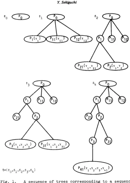
systematically. Let us call such a tree a ~;election rule. If a selection rule is given, a sequence of trees can be defined corresponding to a s·equence of selected problems(Fig. 1).

Let L( t) 'be the set of leaf nodes in t and Ze:: IT be the set of all sub-problems, which can be solved with greatly less computational requirement than Po or which are recognized as ones whose solutions are trivial. Assume BR

can replace Po by a desired set

T

of subproblems in f1ni te iterations.

T

is called a terminating condition. In other 'words, Z is a set of subproblems which an algori.thm designer determines sh:luld be solved without replacing it into finer sub:problems, and T shows the s:itisfactory degree of fineness of search. A prope·r combination of a branchi:ng rule, a selection rule and a terminating condition can generate a finite sequence of rooted trees. t-( to t tIt

t

2 •••••

t

n

)

suer.. that

T4 to=({Po}'~) and t_i li=1.2 ••..•

n)

satisfy Tl through T3, T5 IL(t

i ) -

{L(ti)nL(ti+l)}I=l

(1·1

is the cardinarity of a Sdt).

T6 L(t )e::T. n

72 Y. Sekiguchi

to

C2Q:)

Fig. 1. A sequence of trees corresponding to a sequence of selected problems PO' P

l, P2, P3, P

4

T={PU,P12,P2l,P3l,P4l}'

and

We call each ti in t a search tree and t a search tree sequence(STS). Notice that the problem in the set L(t.) - {L(t')nL(t. l)} is the i-th branched-from

~ ~ ~+

node. T6 represents the state of a search at termination. Remember that elimi-nation, i.e. discarding some of generated subproblems from further considera-tion, has not been referred to, yet. T6 shows a special case of termination.

Complete enumeration algorithms can be reconstructed as a combination of a selection rule, a branc:hing rule and a terminating condition, where

T=Z.

They generate STS's systematically. Many implicit enumeration algorithms can also be recognized as improved versions of such combinations. Before going through detailed discussions of such algorithms, an example will confirm the concepts introduced up to now.

Framework o/Combinatorial Algorithms 73

Example

;~.

Active feasible schedule enumeration in job-shop

An algorithm generating all active feasible schedules for a static jClb-shop scheduling problem with V machines and W jobs, presented in Baker[2]. is restated along the line stated above. Notations needed for describing the algorithm are defined first{ see for detail[2]). O={l,2, ... ,n} is the set of operations to be scheduled and

Yk={(il,ll),(i2,t2), ... ,(ik,tk)}

is a partial active schedule, where

{i

l

,i

2

, ... ,i

k

}

is a set of operations already scheduled

and tj is the completion time of operatlon

i j"

'Ok

is the set of operation!! not contained in

Yk; 'Ok=O-{il, ... ,i

k

}. P

k

is a problem of enumerating all active

feasible schedules which are made by concatinating schedules of

'Ok

to Yk' Le. completions of Yk'

Rk

is the set of operations in

'Ok

whose predecessors are all in Yk' Let 1/1. be the earliest completion time and o. the earliest starting

J J

time of operation

j£'Ok

under Yk'

m(j)

and r(j) are the machine and the pro-cessing time required by operation j , respectively. In the followings, -+-- and -+ imply sub3titution and implication, respectively.

(algorithm)

Step I

Step 2

(preparation)

NO=L(t

_o)

+- {Po}" EO=YO - - <p,

i

+- O.

(selection) Select the first gEmerated subproblem in L (t i)' Let P k be the selected one.

Step 3 Let IjI*=min{1/Iq

I

q£R

k

}

and

m*=mij*),

where

j*dj£R

k

I

1/Ij=1/I*}. DefIne

Step 4

L

as

{jERk

I

0j<1/I*,

m(j)=m*}.

(branching)

BR(P

_k

)

+-

{P

_k+l

I

Y~:+l=YkU(j'Oj+r(j»,

JELl.

(growing)

_{Ni +l}

+-

NiUBR(P

k

), Ei+l

+-

EiU{(Pk,Pk+l)

I

Pk+l£BR(Pk )},

U

L(t

_i

₊₁₎

+-

_{(L(ti)-{Pk}) BR(Pk ),}

where

ti+l=(Ni+l,Ei+l)'

(termination) If

k=n

for all Plc's in

L(t

i

+

l

),

terminate. Otherwi:3e,

go to step 2 after

i

+-

i+l.

Remarks on example 2

1) X

for the problem is the set of all !Lctive feasible schedules and

X(P

_k

)

is the completion set of Yk'

2) A partial schedule Yk is a branching history. If ILI=l for a

P

_k

' IBR(P

_k

)

I =1 and

_{X(Pk)=X(P k+}

I ). But notice that Yk~Yk+l' This implies

Pk+l

is solved more easily than P

_{k ,}

because l'Ok+ll<I'Ok

i

3) Step 2 is a selection rule and (branehing) in step 3 is a branching rule. Let T=Z, where Z is the set of all P (the solution of P is trivial). Then,

74 Y. Seldguchi

Step 4 can be represented by using a condition

L(t.

l)C T.

1.+

4) It will be easily understood that t=(t

O'tl't2' .••.. ) is STS.

3. Tree programming formulation

This section gives a formal description of tree programming. The name stands for the fact that the algorithm generates STS systematically. ThE! validity of tree programming is discussed in the succeeding section.

Recall that a branching rule is a mechanism which replaces a problem with a set of subproblems with additional information y, Le. a branching history. We start by defining such information. Let y be (a sequence of) information which restricts the domain of search to be considered further within a subset of

X,

or which is useful in solving P . p(y) is defined as before(cf. (2.4)).

o

r(~e:r) is a set of y's. r may include infinite-length sequences. r*c r d.enotes the set of maximal sequences among finite-length ones, Le.

(3.1)

r*={YEr

1 1

{y}

1<+00,

yc;.:y' for any y'Er-{y}}.

Corresponding to rand r* , define nand Z as the sets of subproblems emerged by YEr and YEr* , respectively, 1. e.

(3.2) n={p( y) 1 YEf}, Z={p( y) 1 YEr*},

Let A be the class of indeJlendent sets in n(Ac n is said to be an independent set in n i f yq;y' and y'c;.:y hold true for any pair, p(y) and P'ty'), of elements in A).

n(Le. r) is assumed to satisfy two conditions below.

(a)Z is a set of trivial problems. PEn is said to be trivial if (the designer of an algorithm Judges tha'~) P can be solved by a proper procedure and does not need to be decomposed :into finer subproblems.

(b)A mapping BR : n-Z -+

A

exists and satisfies Bl through B4(P

i=p(Yi))' Bl U{X(p)

I

PEBR(Pi)}=X(P

i )·

B2 (I1'PEn-{p_o}) (3 p 'cn-z) (PE8R(P')).

B3 (lifp(y )EBR(P i)) (y i;tY). B4 (lifpEn-Z) (IBR(P)

1<+00).

BR is an abstract expression of branching rules in the previous section. Bl requires that any part of 1~he domain of search never be cut off by BR, more-over it implies the satisf:ication of 1I2 and 113. X(p)'s are not needed to dis-joint each other. But, it :Ls known that BR's which disjoint X(p) 's usually sharpens tree programming ( Bee Balas [3] ). Notice also that X(P )=X(p') can happen for P'EBR(P). B3 requires that the generated subproblems must have more information than their parent(P'EBR(P) is called a son of P and P is said to

Framework of Combinatorial Algorithms 75

be a parent of p'). The definition of A, with B3, ensures

n.

The readers "ill easily understl:tnd that the elements in IT can be arranged in a tree where a branch from ph) to P'(y') corresponds to the relation P'eBR(P). This tree satisfies Tl through T3. Denote as

t

a subtree of this one satisfying the flame conditions. Le-~ ::: be the class of

t'

s (including the original one).

A selection rule is defined as a mapping SR :

A -

II-Z such that 81 (tJAeA) (SR(A)eA), and

82 : ("A,A'eA) (SR(A')eAe:A' - SR(A)=SR(A'».

That the range of SR is II-Z corresponds to T5, and 82 is a consistency condi-tion of SR, L'e. i f a problem in A(e: A') is selected among problems in the larger set

A',

then the same problem must. be selected among problems in A(ef. Fig. 2).

A terminating condition T can be defined as a subset of II, Le. Te:II, as in the previou:3 section. If a combination of SR, BR and

T

is proper, a ST8 satisfying T4 through

T6

will be given by starting with to=({P

o},$) and by repeating SR and BR alternatively(cf. remark

6

on the definition of tree pro-gramming) .

A'

SR(A) • SR(A')

Fig. 2. A schematic representation of 82.

Most enumerative algorithms have sYBtematic fat homing devices. Fathom:~

is to examine generated subproblems and to explore subproblems proved not ~o

have valuable feasible solutions. A subproblem is said to be fathomed if H is proved not to have valuable feasible solutions. Fathomed subproblems can be excluded from further consideration. Mechanisms for fathoming and excluding subproblems are called eliminatiQn rules. An elimination rule is a mapping ER : :::xA - A such that

El : ("t=(N,E)e:::) ("Ae:LCt» (ER(t,A)e:A),

E2 : _a X*e:U{X(p)

I

PeA} -- X*e:U{X(p)

I

PeER(t,A)} and E2s: X*nU{X(P)

I

PeA}

'f:

$ -+- X*nU{X(p)

I

PeER(t,A)}

'f:

$.

76 Y. Sekiguchi

E2a requires that any optimal solutions never be lost in all optimal solUtion cases. E2 requires that '9.t least one optimal solution must be in the

re-s

mainder

ER(t,A)

in single optimal solution cases. For purposes of convenience,

ER

is said to be an identity mapping if

ER(t,A)=A

holds true for any

t=(N,E)eE

and A c: L (

t ) .

The last constituent to be defined is a device to preserve the best solution found out so far. For this purpose, we define an upper bounding func-tion as a mapping u: IT -+ E (E={reals}U{+~}) such that

U(p)= {f(X(P))

f( x) for some known xeX( p)

nF,

or +~

i f PeZ otherwise. The definition in (3.3) i13 stronger than one for an upper bounding function U

g of a lower bound test(cf. section 5) and u is usually used as U

g'

Each definition above is simply a formal description of a elemental func-tion commonly necessary for enumerative algorithms. They are not abstracfunc-tion of constituents of conventional algorithms. This is a distinctive feature of our approach, compared to the preceding researches[1,3,5,6,9,lO,12-14 etc.], where abstract models of conventional algorithms were developed. Further speci-fications of each constituent will be given as sufficient or necessary ~on­

ditions for tree programming having some properties(e.g. [22]).

It is now possible to define tree programming in a general form. T:'J.e indexes, s and a, designate single optimal and all optimal solution cases, respectively. X and ER mus,t satisfy Al and E2 with the respective index. I denotes the best sOlution(s) obtained so far, i.e. incumbent(s).

z

deno~es the value of the objective function for ftel.

Ai

is the set of subproblems in L

i

,

which are not eliminated ; .. hen the i-th selection is implemented, Le. ~~tive

node set. If the initial incumbent ftO is not known at step 1, let f(fto):·+~' As before put

ti=(NiJE

i ) and

t=(t

O

,t

l

,t

2

, ... ).

Noticing the fact that the effect

of elimination rules is only to prune search trees, t of a tree programming

TP

can be said a STS if

TP

is finite. The name tree programming stands for this fact. The sequence of active node sets (SAN) is defined as A(TP)=(AO,A

l " ... ). The sequence of selected nodes (SSN) is defined as S(TP)=(P

O'Pl,P2, ... ). Notice that SAN and SSN are uniquely determined by

t,

and vice versa.

Some-times, the set of subproblems which are surely eliminated in

TP

is implicitly known. This set is referred as V-set of

TP,

and is denoted as V(TP).

vCrp)

is assumed to include all descendants of P if PeV(TP). Consider a branch-and-bound algorithm in which ~jR is the best bound selection type. Subproblems with lower bounds greater than f(X(p )) are surely eliminated. Then, V(TP) for this

o algorithm is equal to {Pen

I

g(P»f(X(P

o))}' see section 5 for

g.

V(TP) of a dynamic programming algor:l_thm with the breadth-first selection can be

identi-Framework of Combinatorial Algorithms 77

fied, too. General cOIllll1ents on the definition below will be given afterword.

[ TP

=(SR ,BR ,U ,ER ,T) ]

s s

single optimal solution cases

Step 1 (preparation) NO=Lo=Ao -+- {Po}' EO -+-

cP,

I -+-XO' z _{-+-f(xo )' i} -+-

o.

Step 2

Step 3 i)

ii)

(branching) B. -+-BR(P.).

1, 1,

(jncumbent) I f

1<2,

then 2 .... -

1

and I - !t. Here, !=min{u(P)

I

PEB

i }, and XEX(P)nF such that PEBi and f(x)=!.

iii) (growing) N. 1 - NYB., L. 1 -+- (L._{P.})UB.,

1,+ 1, 1, 1,+ 1, 1, 1,

U

Ei+l -+- Ei {(Pi,P)

I

PEB_{i },} and let ti+l=(Ni+l,Ei+l)·

U

(elimination) A. l-+-ER (t.+l,(A.-{P.}) B.).

1,+ S 1, 1, 1, 1,

Step 4

Step 5 (termination) I f A. lC:::T, terminate. Otherwise go to step 2 after

1,+ i -+-i+l.

In many practical situations, it is sufficient to get a single optima.l solution. But, if all optimal solutions are wanted, use

TP

for

TP .

a s

[ TP

=(SR,BR,u,ER ,T)

a a

Step 1,2 and ::I i) are the Step 3 ii) : (incumbent)

all optimal solution cases

same as in

TP .

s

I f

j'<2,

then 2 -+-! and I -+-

X.

If !=2, then

I

-+-

IUX.

Here, !=min{u(P)

I

PEB

i }, and X={XEX(P)nF

I

PEBi , f(x)=!}. Step 3 iii), 1, and 5 are the same as in

TP .

s

Remarks on the definitions

1) Th~re are Dlany researches or surveyes(cf. references) on kinds of enumera-tive algorithms and various formalisms are proposed. The definitions here is similar to that of Kohler and Steiglitz[13,14], Geoffrion and Marsten[5] and Baker[2] in the sense that eliminations are done right after branchings. In another class of definitions[Ibaraki 9,10], eliminations are done right after selections and the candidate to be eliminated is only the problem just select-ed. Relations among these formulations are discussed in [24].

2) In a concrete algorithm, it may be trivial from the property of the branch-ing rule that some of the problems in B.(e.g. see example 5 and

6

in section

1,

5) do not need further considerations, or that they are infeasible. In such cases, the whole or a part of ER becomes a formality. But, problems to be

eliminated are rarely known previously and ER is usually given as a procedure for testing ea.ch active problems. Results of the test depend on a search tree at the time of' the test implementation.l"or example, a lower bound test can not be successful before the first feasible solution is obtained. Therefore,

ER

was

78 Y. Sektguchi

defined as one that depends on

t

as well as

A.

3) There are many cases \i'here memory space and computation time are restricted. In order to treat such ca,ses, define terminating conditions as 3-tuple (T,M,C)

where

M

is the maximal allowable memory space and

C

is the maximal allowable computation time(see [14] for detail).

4) Each operation is definitely separated from the others in the definitions. Practically, i t sometimes happens that the amount of computation distinguish-ably increases if all computation concerning to an operation is gathered at its position in the definitions, or that the computation at step 3 ii) is almost the same as the one in step 4. The main purpose of the general defini-tions is to obtain systematic aspects over various enumerative algorithms. To give universal guides for getting an efficient computer program of a solution algorithm for a certain ~roblem is out of the scope of the definitions. In the author's opinion, before going on to designing a program of tree progrlumning, the combination of its constituents should be considered by referring ";0 general properties of tree programming derived under general definitions(see [9,10,13,14,22] as examples of such properties). The similar idea is given in IV of [5].

5) A morphological scheme of various implicit enumeration algorithms i13 given in Mliller-Merbach[19], where conventional algorithms are classified from fifteen different view points. Each of those fifteen classifications can be recognized as a classification of one of five constituents in

TP.

6)

Notice that i f ER is an identical mapping in

TP

and i f T=Z, the

IP

is a complete enumeration algorithm(compare

TP

to example 2). Complete enumeration algorithms here terminate when all leaf nodes are active and in Z. They are different from usual ones that terminate when all leaf nodes are elimina.ted. In this paper, such algorithms are recognized as implicit enumerations with a primitive lower bound test. This kind of

TP

terminates when one subproblem

s

is active and included in Z, even if T=Z. This subproblem gives an optimal solution in

I,

and in actual places it can be eliminated also. But thin must not be done under the definition of elimination rules here. One of merits of our definition is explained in remark

6

of chapter 4.

7) Subproblems in

V(TP)

as well as ones in

Z

are never selected.

Z

can be understood as an expression of algorithm designer's judge on which proll1ems are directly solvable.

V(TP)

is a proved effect of a constituent combination, especially of SR and ER. This is the reason why they are distinguished. On the other hand, a subproblem in

T

may be selected. For example, in a guaranteed accuracy algorithm(cf. example 3 in chapter

5)

with a depth-first selection, P such that g(P»(l-~)z can be selected. This is an essential difference from

Framework of Combinatorial Algorithms 79

the guaranteed accuracy algorithm in [l~)], where approximation is done through a modification of the lower bound test. If T is fixed to Z, approximationB by the terminating condition can not be explained. Notice that the effect of approximation.3 by T on the complexity of' computation is different from that of approximation.3 by the lower bound test. Notice also that subproblems in V(TP) are not sol va'ole and can not be included in Z.

8) Readers ma:r claim that V(TP) of the branch-and-bound algorithm with the best bound selection can be included in T, Le. T=ZUV(TP). If this was done, no subproblem is eliminated by the test. Thus V(TP) must be empty by the defi-nition, and we must understand that T i,; put equal to ZUT

1, where Tl={Pe:1I

I

g(p»f(X(p ))}.

This

T

corresponds to the case (4.6a) or (4.6c), see remark

5

o

in section 4.

4. Validity of tree programming

Here are discussed

(1) under what conditions finiteness of tree programming is proved, and (2) under what conditions tree programmi.ng terminates with optimal solutions. First, the former is discussed.

Let N(TP) be the number of selected nodes at step 2 in TP for a we:n until

the TP terminates, Le. the length of SBN. TP is said finite i f N(TP) is finite for any we:n.

Theorem

1.

Let TP=(SR,BR,u,ER: identity, T), TP'=(SR,BR,u,ER', T) and TP"=

(SR,BR,u,ER',1"'). Assume TcT'. Then, (4.1) and (4.2) hold true. (The

super-fixes below imply the correspondence to TP's with the same supersuper-fixes.) (4.1) (o'P'.e:S(TP')) (3p .(.)e:S(TP)) 1. J 1-((Pi=Pj(i)),,(i~(i) < j(i+l)),,(AiC:: A k, k=j(i-l)+l,. ,J{i))) (4.2)

(lfp'~

e:S (TP" )) (( p'!=P

~

) A

(A'~=A

'.) ) 1. 1- 1-11 1-

1-Proof: (by induction) Notice that PO=P

O because Ao=AO~Po}' and

therefore Ai C::Al· Assume (4.1) holds for i=Z-l(O<Z). I f PZ=Pj(Z_l)+l,the proof

of (4.1) is completed. So assume PZ#Pj(Z~l)+l' Notice that AZ_l c::Aj(Z_l) B.nd that ER is an identity mapping. Necessarily, AZCAj(Z_l)+l' Therefore, if TP

is finite, Pj(Z-l)+<l(=PP must be in S(TP). Let Pj(Z_l)+o(O<<l) be the firs·t

element in S(TP) such that _{Pj(Z_l)+oe:A Z'} Then, both Pj(Z-l)+O and Pj(Z-l)+<l are included !,n _AZ C::Aj( Z-l)+o' and _{SR(AP#SR(Aj ( Z-l)+O)'} This contradicts to S2. This impl:~eB that AiC::Aj(Z_l)+jJ(l~';;fL) must hold. As a result, (4.1) holds

80 Y. Sekiguchi

for i=l. This completes the induction for (4.1).

Notice that

P"=P'=P

_{0 0 0} and

A"=A'={P}

_{0 0 o '} Assume (4.2) is true for i=l, then we see that BR(~~(Al))=BR(SR(Ai)) A1+l':ER( tl+l

,A)=Ai+l

SR(Al.+l )=SR(Az.+l ) (step 3 i)), (step 4) (step 2).

is established by induction. This terminates our proof.

Corollary 1.

N(TP')<+oo -+- N(TPII) ~N(TP') ~N(TP)

Proof:

Immediate from theorem 1.

and

Finiteness of

TP

is established if it is shown that SR emerges a finite sequence of selected nodeB, which leads to an active node set included in

T.

Leaf nodes not included in

T

at the termination must have been eliminated. But notice that a subproblem is guaranteed to be eliminated only when it is included in V(

TP).

ConverBely, subproblems not included in

V(TP)

mayor may not be eliminated. Thus, the effect of ER on finiteness is condensed into

V(

TP).

Moreover, subproblems are generated by

B/1.

It is natural that the cond-itions for finiteness are expressed in terms of SR,BR,T and

V(TP).

Theorem 2.

If conditions 1, 2 and

3

hold true for any

WEn,

then

TP

is finite. [cond. 1] [cond. 2] [cond. 3]

(4.3)

('o'PET-Z) (BR(P)C:

rUV(TP)).

(SR(A

i ) ET-Z) -+- (3n<+oo) (SR( Ai+n) iT-Z) .

(3m<+oo) (Bltn(Po)C:TUV(TP)), where

BRO(P)=P

BRi+l(p)={P'EBR(pII ) PIIEBRi(P)-ZUV(TP)}U{BRi(P)n(ZUV(TP))}.

Proof:

Let

A=A.-TUV(TP)

(~~)

for i<+oo. By condition 3, any

PEA

must fall

1-into TUV(TP) in finite iterations of BR. Because if PET-Z, all descendants of

P

must be included in

rUV(TP)

by condition 1, and because

IAI<+oo

by B4, the proof is completed if it is shown that

PEA

and its descendants included in

II-TUV(TP) are selected wi-:hin finite iterations of step 2. Notice that

SR( A) EA-TUV(

TP)

or SR(A) ET-Z.

Because the latter never eontinues infinitely by condition 2, the former, i.e.

SR(AhII-TUV(TP) must happen any desired time within finite iterations of step

2. This completes the proof.

Remember that X is allowed to be an infinite set. If we are not lti.cky enough to find a branching rule ·",hich generates only finite-length inforlnation

se-Framework of Combinatorial Algorithms 81

quences,

r

includes infinite-length ones .. The infinite-length sequences co:rres-pond to infinite-length paths in a search tree. By the definition, Z can not include subproblems definied by them. Such subproblems must be included in

(T-Z) UV( TP) i f TP is finite. As mentioned in remark 7 of the preceding cha:[lter,

subproblems in T-Z can be selected and branched from. Thus, finiteness in the sense of parallel operations(condition 3.1 is not enough. Tree programming is a sequential alg::Jrithm and additional cond:~tions 1 and 2 must be satisfied. In other words, c::Jnditions 1 and 2 are needed to prevent tree programming from cyclig or zig-zag operations around TUv("rp), which may happen by chance. An example of zig-zag operations is shown in Fig. 3. In the figure, P. is the i-th

1-branched-from subproblem. Suppose that SR of a TP continues to select subp:ro-blems in the two tails starting from P

6 and P7, and that these tails are of infinite length. Then, TP can not terminate, because the left most subprob.Lem in BR2(P ) _o has not been branched from yet and is not included in

TUV(TP).

If

T

is larger than Z, TP is usually an approximate solution algorithm. Corollary 2 states that finiteness in the sense of parallel operations is sufficient for TP with T=Z to be finite, and corollaly 3 tells us that testing satisfication of condition 3 under T=Z ill a cheap method for establishing finiteness of TP with

T

larger than Z.

Corollary

2.

Let T=Z. If condition 3 holds true for any WEn, then TP is finite.

Proof: Immediate from theorem 2 and the fact that conditions 1 and 2 are trivially satisfied if T=Z.

Corollary 3. If the condition 3 ho:_ds true for T=Z and for any WEn, then TP is finite for any

T

including

Z.

Proof: Immediate from corollary 1 and 2.

Generally speaking, subproblems not in V(TP) can be eliminated and the condition 3 is not a necessary condition. But, if V(TP) is the set of sub-problems possibly eliminated(see [22] for such cases), the condition is neGes-sary for finiteness.

Theorem

3.

Let TP satisfy condition 1, and assume P is eliminated i f and only if PEV(TP). Then, if N(TP) is finite, condition 3 holds true.

Proof: let N(TP)=m. Then, Am+l c::T. Define n_l as

~=max{q

I

PEB~(PO)' PEAm+l}·

Let

A=

Lm+l-Am+l. By the assumption on V( TP), AC::V( TP). Define n

2 as

n

2=max{q

I

PEBR1 (PO)' PEA}. By comparing the definitions of N(TP) ani BRq(P

82 Y. Sekiguchi

j'l

BR 1 (PO) BR2(P O}

,

,

\ I \

,

_\

©

Fig. 3. BR3(P 0)

Gp'S

in V(TP)

o

P's in T-Z

@

P's in Z A schematic representation of theorem 2. m+l and n2~m+l must hold. Let k=max{~,n2}' By condition 1, we get

BRk(Pa)c:. TUV(TP).

By theorem

3,

it is realized that the conditions in theorem 2 might be the weakest one. Notice also that condition 3 with T=Z and V(TP)=4> implies finiteness of YEr. If IXI<+~, condition 3 can be altered by condition 4.

[cond. 4) (liPEn )

(3n<+~)

('!fp, EB~(P)) ((X(p') ~X(p)) V (p' ETUV( TP)))

If the part X(p')~ X(p) 1.ere not in condition

4,

it is essentially equivalent to condition

3.

The next lemma implies that condition

4

together with condition

1 guarantees satisfication of condition 3 for subproblems with a finite domain of search.

Lemma 1. I f conditions 1 and 4 hold true, for any PEn it holds that

IX(p) 1 <h -+ (3 m<+=)(Bff1(P)c:. TUV(TP)).

Proof: Let P be an arbitrary one in

n.

If PEZ, the lemma trivially holds true for

/'/Fa.

Assume P En·- Z. Condition 4 requires the existence of n<+~ such that

Framework of Combinatorial Algorithms

because X(P) is a finite set. Again, by condition 4 every P' EU(P) must fall into TUV(TP) in finite iterations, i.e. there must be a finite V such that

BRV(P')e:: TUV( TP).

Let m*=max{v \ P'EU(P)}. m* is well defined because \B~(P) \<+w by B4. By condition 1, BRq (p) e:: TUV( TP) forq=n+m*. rhis completes the proof.

83

Notice tt.at lemma 1 implies satisfication of condition 3 , if X=X(p ) is o a finite set. Therefore, conditions 1, 2 and 4 ensure finiteness. This fact is given in theorem 4 in a slightly generalized form.

Theorem if. Assume conditions 1, 2 and 4 hold true for any wdl. If the next is true for any WEn, then TP is finite.

(4.4) (3m<+w) (IU{X(p) I PE~}I<+w).

Proof: (4.4) implies that Ix(p) I<+~ is true for any PEAm' By lemma 1, we can define a finite q(p) for each PEA, 'where

m

q(P)=min{q I B~(P)e:: TUV(TP)}.

Notice also that I A I <+w by B4. By doing almost the same as in the proof of

m

theorem 2, N( lP) <+w is established for each WEn.

Corollary 4. Let IXI<+w. I f condition 4 holds true for T=Z and any WEn, then, TP is finite for any

T

including Z.

Proof: If Ixl<+w, TP' with T=Z ter:ninates in finite iterations under condition 4. (We can get a corollary of theorem 4 similar to corollary 2 of theorem 2.) Use corollary 1 in establishing finiteness for an arbitrary (Ze::)T.

Now that the conditions for finiteness were clarified, we proceed to the correctness. Recall that equations (4.5) hold true for i=O.l, •••• n(n=N(TP))

by the definitions of ER and step 3 ii). (4.5a) Z ~ min{ u(p) I PEA

i }

(4.5b) U{X(p) I PEAi}nX*:f <p

x*e::U{X(p) I PEA.}

'Z-for both TP and TP .

for TP . s for TP .

a

a s

Theorem 5. Let TP=(SR,BR,u,ER, T=TIUZ), then equations (4.6) hold true at

the termination, where Xi is defined by

I: 4.7) .

(4.6a) X* :f x* ~ _{X*-Xi e::I for TP .}

1 a

(4.6b) X* = X*

-..

f(X(P

o)) :;"

Z ~max{u(P) I PET

1} for TP . 1 a (4.6c) X* ₁ 4>

-..

InX* :f 4> for TP . _s (4.6d) X* :f <p --+- f(X(p 0)) ~ Z ~ max{u(P) I PET 1} for TP . 1 s (4.7) X*=U{X(p) 1 I PET1}n X*

84

Proof:

Y. Sekiguchi

For TP , A c=T and (4.5c) imply that a n

X*-X* C {X(p) I PEA -T

l } and A -Tlc Z .

.1

n

n

By step 3 ii), all optimal solutions in An-Tl must be conserved in I, Le. (4. 6a) must be true. f(X(p 0) );;'2 is trivial and if Xi=X* we may not get any optimal solutions before termination. But from (4.5a), it is true that

2;;' min[min{z,,(P) I PEAn-T_l }, min{u(P) I PEAnnTl}] ;;. max{u(P) I PET

1}·

This establishes (4.6b). (4.6c) and (4.6d) can be proved similarly.

I t may seem peculiar that the condition for single optimal solution cases is more strict than the one for all optimal solution cases. As an explanation, remember that ER in TP may eliminate all but one opt imal solutions. I:' the

s

remaining optimal solution is in Xi, no optimal solution may be obtained. The next corollary is immediE.te from theorem 5 and gives a condition for correct-ness of tree programming.

Corollary 5. I f T=Z, then tree programming is correct, i.e. I=X* for TP

a

Remarks

on

the results

and for TP .

s

1) Corollary 1 for T'=Z gives a comparison of computational requirements among an exhaustive enumeration(TP), an implicit enumeration(TP') and a kind of ap-proximate enumerations(TP"). Theorem 1 shows the tighter relations among them. See also remark 5, below.

2) The conditions 3 and l~ with T=Z and V(TP)=<P are the sufficient conditions for finiteness of exhaustive enumerations with an infinite and a finite do-mains of search, respect:~vely. See corollaries 2 and 4.

3) As an example of theorem 2, ER in cutting plane methods(cf. example 6 in the next section) eliminates P i f and only if PEV(TP) (=the set of infeasible problems). The proof of finiteness of the methods is completed by showing that Po falls into Z (=the Bet of linear programming problems having integer optimal SOlutions) in finite iterations of cutting plane generation.

4) The larger the size of V-set is, the smaller the maximum computational re-quirement will be. Notice that eliminating subproblems in V-set is equivalent to or more than enlarging the terminating condition from

T

to

TUV(TP),

and that theorem 1 indicates the tendency above. Because one of the difficulties of implicit enumeration algorithms is the tendency that they may reduce to exhaustive enumerations, the concept of V-set is very important. Irr-ZUV(TP) I is the possible maximum 'Talue for N(TP). If this cardinarity is small enough, tree programming can be a polynomial time algorithm. Johnson's rule for two

Framework of Combinatorial Algorithms

stage flow sho:;> scheduling problem can be recognized as an example of this sort of tree programming.

85

5) Theorem 5 S:10WS that introducing Tl makes tree programming a sort of ap·· proximate algodthms. In cases of (4.6b) and (4.6d), i f max u(p) over Tl i:, estimated exli!~itly, tree programming is" so called, a guaranteed accuracy algorithm(see [14J and example 3 in the next section). If Tl is made sure previously that it is the case of (4.6a) or (4.6c), it is natural to expect that the subproblems in

Tl

can be included in V-set and that

T

can be put

Z.

6) In all the tree programmings discussed up to now,

T

was equal to or larger than Z. We can suppositionally regard I as a set of trivial problems. Notiee that I always !~ontains the best solutions in

AiOZ,

Hence, practically every subproblem in .z can be eliminated by using the lower bound tests(cf. example 3), and we can put T=T

l . But, to do this is to violate E2, and then E2 must be slightly modified. Notice that if this was done, T=cp in example 6, and tree programming can not include cutting plane methods, because their

ER's

does not include the lover bound tests.

5.

Illustrative examples

Branch-and-bound mehtods, the additive implicit enumeration, cutting plane mehtods and dynamic programming ale;;orithm are reformulated as specia:. kinds of tree :9rogramming. The purpose here is to show the universality of tree programmi;1g concept over a wide variety of algorithms. See example 2 for an exhaustive ,=numeration, where

ER

is an identity mapping.

Models in [5J and [17] do not contain other dominance tests than lower bound tests. T::1ey can not represent example 4. The model in [13J do not inc:lude feasibility te:3ts and can not explain example 6. Moreover, this model is only for permutation problems. Ibaraki's model seems most flexible. But, it can explain neithe:~ analytical solutions(cf. remark 4 in the preceding section) nor a guaranteed accuracy algorithm in example 3. The method in [12] will be explained within tree programming framework, too. Example 5 can be explained by anyone of these models. This algorithm has many variants, which are uS\lal1y distinguished from branch-and-bound methods(e.g. see p. 210 of [20]).

Example 3. Branch-and-bound methods

In recent papers[lO,13,14J, a genera.lized or abstracted version of the: hybrid dynamic programming/branch-and-bound algorithm(DP/BB) in example

4

h also called "branch-and-bound method". Such version is also regarded as trEle programming(cf.[24J). Here, we use the term "branch-and-bound" as the one j.n

86 Y. Sekiguchi

the sense of Little et al.[16], Balas[3], Mitten[17] and Ibaraki[9]. A lower bounding function is a mapping

g :

IT -+ E such that

g(p)

{=

f(X(p)) ~ f(X(p))

for PEZ

otherwise. An upper bounding function of the second type is U

g IT -+ E, such that.

(5.2) ug(P) {= f(X(p)) for PEZ

~ f(X(p)) otherwise.

Let Zg=+oo at step 1, and assume that Zg is updated by (5.3) after each branch-ing operation, somewhere between step 3 i) and step 4.

(5.3) Z =min[z , min{u (p)

I

PEA.}].

g :1 g

'l-Obviously, f(X(Po))~Zg and g(P)~(X(PO)) hold true. Then, an elimination rule which consists of a lower bound test can be defined as a mapping ER :

=xA

-+

A

such that i f ER(t,A)=A', then

( (V'PEA')

(g(P)~Zg))

A ( (VPEA_A') (g(p) >Zg))

«V'pe:A'_P*) (g(:?)<Zg)) A«V'PEA-A')

«g(P)~Zg)A(PtP*)))

for ER a for ERs' where P* is a singleton set of a subproblem which has given the current value Zg.

As simple upper bounding functions, we can use the following one. for PEZ

U(P)=Ug(P):: {g(P)

+00 otherwise.

Then, i t is easily realized that

TP

with ER defined above (notice that z=z in

g

this case) is a branch-and-bound method in the sense used here. The definition (5.1) is similar to the one in [9] and [17

J.

Lower bounding functions are often restricted by the third condition;

g(p)~(p' ) i f X(p')C::X(p).

Making g satisfy this condition is very easy in practice and it makes ER more powerful. But this condition is not needed for the object here.

In order to get a guaranteed accuracy algorithm, let, as an instance[14],

It is known also that the better the initial incumbent is, the less the compu-tational requirement is[ll.].

Example 4. A hybrid DP/BB algorithm[18]

We consider a discrete multistage decision problem with an additive ob-jective function.

S

is the finite set of all feasible states.

D

is the finite set of all possible decisions.

T: SxD

-+

S

is a transition mapping, whi~h

means if a decision

dED

is implemented on a stage with a state

SES,

the state on the next stage is

T(s,cl). A(s)={dED

I

T(s,d)ES}

is the set of all feasible decisions at a state

s.

y is a sequence of decisions;

y=(d

l

,d2, ... ,dn),

l~n. For simplicity, if a state s' results from y implemented in its sequence on a

Framework of Combinatorial Algorithms 87

state s, denotE! T(s,y)=s'. a(s,d) represents an incremental cost when d is implemented on a state s. SOES is an initial state and Se cS is the set of feasible final states. Then, a data which describes a problem is the set

w=

(So,S,Se,D,T,a). Let X and F be the set of feasible decisions which make mcves from So to SES-,{SO} and from So to SESe' respectively, i.e.

X={y

F={Y

T(SO,y)ES-{SO}' and T(s. 1,d.)=s.ES _'/..- for i=1,2, •••

,n},

'/.. '/..

T(SO,y)ES

e, and T(s. 1,d.)=s.ES '/..- '/.. '/.. for i=1,2, •••

,n}.

The cost of XEX can be represented by f; assume :x:=(d

l ,d2, ••• ,d

n

),

then

f(x)=:

L~=l

a(si_l ,d_i ) ,

The problem actually solved by the algorithm below is (2.2) with the para-meters defined above.

y.y' is a decision sequence where y is followed by y'. Let ~(y) be the set of decision sequences which can be concatinated to y; 1'( y)={y'

I

Y'y' EX}.

Then, X(p(w,y)) is the set {y.y'

I

y' <.P(y)}. A lower bounding function is defined as

g(p(w,y) )=f( y)+l( y),

[I

y)

r:n(fl

y') under

where

a initial state So

I

y'EF(y), SO=T(So'y)}

i f

yiF,

otherwise. We can put Z={p(w,y)

I

YEF}. Define u(p) and u (p) by (5.4), then g, u and u

g

g

satisfy (5.1), (3.3) and (5.2), respectively. Define the constituents of TP other than u aB follows.

SR : FIFO rule, i. e. select the first generated subproblem in A.- Z. Let '/..

P .(w,y) be the selected one. '/..

BR : BR(Pi((~,Y))={P(w,y.d)

I

dEA(s), ","here S=T(So'y)}.

ER : (5.8)

I f ER( t:, A)=A', then

A-A'=

1

{p(w,y)EA

I

(g(p(w,y))>z)

v( (3p ( w, y') EA) ((T( so,y)'=T( so,y')) flU( y) >f( y')))} {p(w,yhA-?t

I

(g(p(w'Y))~fI)

for TP a

V( (3p ( w,y') EA') ((T( SO' y)=T( SO' y')) fI(f(

y)~

y')))} for TP T=Z·

SR and BR above trivially satisfy 81, 82 and Bl through B4, respeotively.

ER

satisfies El. The remaining to be shown is the satisfication of E2. Notioe that SR selects a subproblem with the shortest decision sequenoe and th&t y'

s.

of P in BR(P( ~), y)) is longer than y Just by one. This means that there appear repeatedly ~'s in which all related y's have the same length

k.

Let

f

k

(

8) be the minimum cost for bringing the system from So to SES by at moat k decisions.

88 Y. Seldguchi

At the instance mentioned above, the following equation must hold for each p( w, y) E:.A ..

1.-(5.9) fk(s)=f(y)=min.:/(y') I s=T(so,y)=T(So'y'), ly'I=lyl=k} =min':fk_l(s')+c(s',d)

I

dE:.A(s'), s=T(s',d), s'E:.B}.

(5.9) is the functional equation of dynamic programming. Thus, ER sathfies E2 and TP with the parameters defined here is really tree programming, a:1d this algorithm is called a hybrid DP/BB [18J. Notice that this algorithm reduces to a branch-and-bound methoc~ i f the last half of (5.8) is omitted, and to a dynamic programming algorithm if z -+ +oo( i. e. the lower bound test is not active). The model in [10,13,14J are regarded as general versions of t:1is algorithm.

Example 5.

The

additive implicit enumeration[4J

The additive implidt enumeration(AIE) algorithm is one for solving 0-1 integer linear programming problems. Define notations as follows.

N={1,2, ... ,n}, M={1,2, .•• ,m}, .:lr(x

l ,x2, ••• ,xn)t, c=(al ,a2, ••. ,an) where

a (qdV) are nonnegative integers, b=(b

l ,b2, ... ,b )t where b (pE:.M) are integers

q

m

p

and A=IIa 11 where a (pEJ.f, qdV) are integers. Let X= {x I x =0 or 1 for qE:.N},

N

N

q

f{ x)=ax and F= {xE:.X I Ax,j)}. Then the problem solved by AlE is defined by (2.2) with the parameters defined above. w here is (N,M,A,b,c). Let P .(w,y.) be the

1.- 1.-subproblem selected as tbe i-th branched-from one. Here, Yi is the branehing

lU 0

history and is defined as the union Yi Yi' where 1

y. the set of qdV already fixed at x =1,

1.- q

o

Yi the set of qE:.N already fixed at xq=o.

The sequence of the elements in y. is not important (but is determined by BR),

1.-and we will treat y. as a set for convenience sake. _{_ 1.-} N.=N-y. _{'!- '!-} is the set of free variables. The domain of search of P.(w,y.) is

1.-

1.-X(P.(w,y.))={XE:.X I x =1 for

qE:.y~,

x =0 for

qE:.y~},

1.- 1.- q 1.- q "/..

We can put T=Z={P(w,y.)

I

the O-completion of y. is feasible}, where the

0-1.- 1 1.- 1

completion of y. is x such that x =1 for qE:.Y., X =0 for qE:.N-y •.• A lower

bound-1.- q 1.- q v

ing function is defined as

(5.10) g(P.(w,y·))=L la x {=f(X(P.(w,y,))) 1.- 1.- qE:.Yi q q 1.- 1.-~(X(p .(w,y.))) 1.- 1.-Define

u

and

u

by g respectively.

(5.4), then

g,

u and u satisfy (5.1),

g

for PE:.Z, otherwise. (3.3) and (5.2),

BR : LIFO rul=, i.e. select the last generated subproblem in A.-Z. 1.-In defining the remaining constituents, notations below are needed.

Framework of Combinatorial Algorithms 89

dp=LqdlCQ; max{O,apq } + Lq e:

Yl

_{apq - bp} for pe:M, ;,here Q~={je:N·la.>z-L l a } .

'/- J= qe:yi q

If d >0 for all pe:M, make Q~ and Q-: as follows.

F '/-

'/-+ {' -

I

d

Q.=Je:J,l·-Qc a·> ,pe:M},

'/- '/- PJ P

. +

-Moreover, lf ~ii=Qi=~' select j* which satisfies

V.*=nlin{V.

I

je:N .. } , where

J J "

Notice that there is no feasible completion of y. if d <0 for some pe:M, that

+) _ '/- P

x =l(qe:Q. , x =O(qe:Q.) are necessary for completions of y. to be feasible and

q '/- e r ' / ' /

-that j* can be regarded as an index for which x.*=l added to y. makes y. near

J '/-

'/-to the feasib:_e one most effectively among the free variables. Thus, we cS.n define BR and ER as follows.

BR : BR(P.(w,y.))={P ,Pal, where '/- '/- Cl..,

1_ lU + 0_ 0u

-YCl-Yi

Q

_{i ,} YCl-Yi

Q

_i

one such that X(P Q )=X(P. )-X(p )

.., '/- Cl P

yl=y~U{j*}, yO=y~

Cl Cl'/- Cl'/-1 1 0 OU{~} Ps YS=Yi' YS=Yi J ( ) A -( )Ll ( )

ER : If ER

t,A

= , where

A-

A.-{p.} BR P. , then

1 7, '/-U{P S

I

Q~UQi

f:

$}U{Pe:A-P*

I

g(p)~z}

{Pe:BR(P i )

I

((~e:M)(dp<O))V(Q+nQ-

f:

~)} for

TP ,

s A_A'=I _{{Pe:BR(P i )}

I

((3p e:M)(d_p<O))V(Q+nQ-

f:

~)}

u{Ps

I

Q~uQi

f:

~}U{Pe:A

I

g(p»z} for

TP

_{a ·}

BR and ER also satisfy Bl through B4 and El, E2, respectively. Algorithm

TP

with the parameters defined above is tree programming. AlE in [4] is different from this algorithm in the point that the test for elimination is done just after step 2 only on P just selected. Notice that the middle part in the right hand side of ,: 5 .11) is a formality, beca.use Ps in the case may not be generat-ed practicall;r. Notice also that all information necessary for ER, except the middle part, (!an be made just from Y of each problem. Therefore, a subprohlem can be eliminated in AlE if and only i f it is eliminated in

TP.

Thus,

TP

is essentially AlE in the sense that the sE'quence of actually branched sub-problems in

TP

is exactly the same as one in AlE, i.e. the STS's corresponding to them are e,sentially the samething(cf. remark 1 in section 3 and [24]) '.

90 Y. Sekiluchi

Example 6. Cutting plane methods

Algorithms for pure integer linear programming problems are treated below. Define

N, M,

a,

b,

a, x and

f

as the same as in example

5.

F

and

X

are defined as

F={x Ax~, x : nonnegative integer for qeN},

q

X={x Ax~, x : nonnegative real for qeN, ax~ax*}. q

Again, the problem actual:LY solved by the algorithm below is defined by (2.2)

"

with the parameters defined above. Let P. be a subproblem of

po(w).

R. denotes

1. 1.

the set of feasible solut:lons of the linear programming problem corresponding to

Pi.

For example,

RO={x

I

Ax~, Xq: nonnegative real for qeN}.

Suppose that a cutting plnne can be produced by a proper method. Cutting planes are denoted by vx=tJ, where V is a lxn vector and ~ is a scalor. P. is

1. divided into P and P a where X(p )={xeX(P.)

I

vx>~} and X(P a)={xeX(P.)

I

vx<w}.

C l " Cl 1. - " 1.

Then, X(P S)nF=~ from the property of cutting planes and RCl={xeR

i

I

vx~~}. A cutting plane method is

TP

with the following constituents.

SR BR u An identical mapptng(A_i BR(P .)={P ,P a}. 1. C l "

u(p)= {min{aX

I

XE:X(P)}

+00

ER: ER(t,{PCl,PS})={P Cl}.

is always a sigleton set).

HPeZ otherwise.

T=Z={P

I

R of P has optimal integer vertices}.

Notice that cutting plane methods search for optimal solutions from the out·-side of the feasible region, and that R used for generating a cutting plane is not the domain of search for a cutting plane method. Research on how to make deeper cutting planes should be recognized as one for better BR and ER.

6. Conclusion

Tree programming has been proposed as a general framework unifying the conventional models. The essential difference from the conventional ones is in the point that the elimination rule is defined as any mechanism which elimi-nates some of active subproblems. The elimination rule will be constructed by combining four test functions[22]. Because of this flexibility, various algo-rithms were shown to be sorts of tree programming. The conditions for finite-ness and correctfinite-ness were obtained for both infinite and finite domains of search. They were given in simple forms and clarify the properties which each constituent must have.