Algorithmic Methods for PH / PH / 1 Queues with Batch Arrivals or Services

Journal of the Operations Research Society of Japan

Vol. 26, No. 1, March 1983

ALGORITHMIC METHODS FOR PH / PH /1 QUEUES WITH

BATCH ARRIVALS OR SERVICES

Yutaka Baba Tokyo Institute of Technology

(Received December 23, 1981; Revised October 13, 1982)

Abstract We discuss algorithms for the computation of the steady state features of PH/PH/l queues with bounded batch arrivals or batch services. Many characteristic quantities such as the mean and variance of queue length in continuous time, the mean waiting time, the waiting probability, etc. are obtained in computationaJIy tractable forms. We also show various numerical values.

1.

Introduction

In most of all studies on the queueing systems with batch arrivals or services, it has been assumed that the interarrival time distribution or the service time distribution was exponential. Then we shall consider here a batch arrival queue denoted by PH[X]!PH!l , in which the distributions of interarrival and service times are of phase type. We only discuss the case that consecutive batch sizes are independent, and have the common probability

{gi}' 1 ~ i ~ K , with mean g, where K is the largest index for which gK >

O.

And we also consider a batch service queue denoted by PH!PH[Y]!l. The batch service discipline is one introduced by Bailey [1]. A server can serve up to K customers simultaneously. At each service epoch, the first K customers in the queue may be received their services. If the queue length is shorter than K, all customers in the queue are served.

Phase type distributions were introduced by Neuts [6]. A probability distribution on (0,00) is said to be of phase type if it is obtained as the distribution of the time till absorption in a finite Markov chain with con-tinuous parameter. The class of phase type distributions includes a number

PH/PH/l with Batch Arrivals or Services

of well-known and important distributions such as generalized Erlang and hyperexponential distributions appeared in the queueing theory, and it is dense in the class of all probability distributions concentrated on (0,00). So the classes of models of types PH[X)/PH/l and PH/PH[Y)/l queues are also tractable for numerical analysis.

13

Recently Neuts [9) showed that an important class of infinite stochastic matrices had an invariant probability vector of a matrix-geometric form. The models discussed in this paper have this property. Based on Neuts's result, we shall obtain many characteristic quantities such as the mean and variance of queue length in continuous time, mean waiting time, waiting probability, etc. These quantities are obtained in computationally tractable forms. We also show various numerical examples and obtain qualitative insight into the effect of varying the parameter values.

2. Preliminaries

In this section, we prepare some notations and basic properties related to matrices and phase type distributions.

We denote by I the identity matrix, by 0 the zero matrix, by 0 the zero vector, and by e the column vector with all entries equal to 1.

In the later discussions we will frequently use Kronecker products of matrices (e.g.,Bellman [2]). Let X

=

(X

i j) and Y

=

(Yi j) be and m x n matrices respectively. Then we denote by X

®

Y

Y Y

m x n x x the Kroneeker product of X and Y, which is an (m m ) x (n n ) matrix whose entry in

x Y x Y

the «i-l)my

+

k)th row and in the «j-l)n

y

+

~)th column is XijYk~. Now we examine some basic properties of a phase type distribution F(x).

Suppose that F(x) is represented by a continuous time Markov chain on the state space {0,1,2, ... ,m} with the initial probability vector

(2.1) 0.0

= (O,~)= (0,o.

l,o.2,···,o.m) and the infinitesimal generator

(2.2) QO =

[:0

!j=

0 0 0 .0 tl qll q12 qlm t2 q2l q22 q2m t _{qml qm2 qmm} m

tran-14 Y. Baba

sient (or nonrecurrent) states. All the entries of aO and off-diagonal entries of QO are nonnegative and Q~

+

~o

=

Q .

The distribution function

F(x)

is written as (2.3)

F(x)

= 1 - ~xp(Qx)~

,

for x ~ O.

The pair (~, Q) is called a representation of

F(o).

We can show that the moments ~k" k ~ 1, about the origin all exist and are given by the formula

(2.4) for k ~ 1

Examples:

(a) For the exponential distribution with parameter A, the matrix Q is given by

(2.5) Q

=

-A

and

so that

F(o)

has the simple representation (l,-A).

(b) The generalized Erlang distribution obtained by the convolution of m exponential distributions with paramete"rs AI" .. ,Am has as one of its representations the pair ~, Q) given by

(2.6) with a

=

(1,0, .•. ,0) Q= -A 1 Al 0 0 0 -A 2 AZ 0

o o

o ...

-A m T (O, ••• ,O,A) • m

(c) The hyperexponential distribution

(2.7)

F(x)

m

L a.(l -

exp(-AiX»

,

i=l ~

x~O

may be represented by a

=

(al, .•. ,a

m) and Q

For any representation a , Q ), we can define a matrix Q* by

where TO (~0,

...

,~0) and AO

=

diag(al, •.• ,a m).

PH/PH/l with Batch Arrivals or Services

m-state Markov chain, which has a close relationship to the probability distribution F(o).

The significance of Q* is as follO\~s. At any time that an absorption occurs in the Markov chain QO, we instantaneously perform a multinomial trial with outcomes 1, .••

,m

and probabilities CL

l, •••

,am

to pick a new initial state. Considering each absorption into the state 0 as a renewal, we obtain a renewal process for which the time between any two successive renewals has cdf F(o), the phase type distribution given by (2.3). Such a renewal process is called a renewal proc,~ss of phase type (Neuts [8]).

The above procedure also constructively defines a new Markov chain with state space

h, ...

,m}, initial probability vector a and infinitesimal generator Q*. This Markov chain describes the "phase" of the system. In Neuts [6], it is shown that one may, without loss of generality, assume that the representation ~,Q of F (0) is so chosen as to make 0* irre'-ducible, and we shall henceforth assume that this is indeed the case.

We let TI denote the stationary vec:tor of the Markov chain 0*, Le., the unique (strictly positive) vector satisfying

.:!!.O*

=

Q , TIe

=

1. I t may be easily shown that TI =

_A~-l,

where A- l =

_~-l~

is the mean of F(o).

3. PH/PH/l

queue

with batch arrivals

Consider the PH[X]/PH/l model, in which customers arrive in batches. We shall assume that the probability dist:ribution F( 0) of the batch inter-arrival times is of phase type with a representation ( i ! , T ), where T is a matrix of order M and that the probability distribution G(o) of the service ~imes is of phase type with a representation (~, 5 ), where 5 is a matrix of order N. Moreover we put. that TO

We assume that consecutive batch sizes are independent and have the common probabili ty function {g, ; 1 < i < K}, w'i th mean g, where K is the

~ = =

largest index for which gK > O.

In this section, we discuss the stationary distributions of the number of customers in the system at an arbitrary epoch t. In order to obtain the stationary distribution of the PH[X]/PH/l queue, we shall consider the continuous parameter Markov chain which represents the transitions of the states of the states of the PH[X]/PH/l queue at arbitrary epoch. In order to define the states of this Markov chain, we shall define that the index i

(i

~ 1) denotes the number of customers in the system, the index j

16 Y. Baba

(1 ~ j ~ N) represents the phase of service process, and the index h (1 ~ h ~ M) represents the phase of arrival process.

Then the PH[X]/PH/l queue may be studied in terms of a continuous parameter Markov chain with state space (QU~), where

Q

=

{(O,h),

1 ~

h

~

M}

and ~

=

{(i,j,h), i ~ 1, 1 ~ j ~ N, 1 ~ h ~ M}. The infinitesimal generator of the Markov chain is given by the matrix

0 1 2 K K+l K+2 K+3

0 _{Co g/)O gio gjJO} 0 0 0

1

_Ba

C

_{glD gK_lD gjJ} 0 0

(3.1) Q

2 0 B

C

_{gX_2}

D

_{gX_l D gKD} 0

3 0 0

13

_{gK_3}

D

_{gK_2}

D

_{gK_lD gjJ}

where

Ba

§...o® I, B

and

D

= I

®

TOAo. I is the idintity matrix of order N when it is in the right of the symbol

®

and the identity matrix of order M when it appears to the left. We see that the dimensions of the matrices Ba, Co' DO are

MN x M, M x M, M x MN, respectively. All other blocks in Q are square and of order MN. It is easily verified that the PH[X]/PH/l queue is

bl 'f d 1 if ' < h ' -1 T-l and j.J -1 _- _os-le.

sta e 1 an on y gAl j.Jl' were Al = -a e 1 ~_

We denote the invariant probability vector of Q by ~,which we may write in the partitioned form {~, ~l"'" ~i""} ,where ~ is M-vector and ~i ' i ~l , are MN-vectors.

The component

xO,h

of ~ is the stationary probability that, at an arbitrary time epoch t, the queue is empty and the arrival process is in the phase state h , 1 ~ h ~ M. The component Xi,j,h

i ~ I, is the stationary probability that there are i

of the vector x. -~ customers in the system, the service process is in the j-th phase, 1 ~ j ~ N, and the arrival process is in the h-phase, 1 ~ h ~ M at t.

Let l be the real number such that

(3.2) l = max[ max {-(CO).

J,

max {-(C).

J]

> 0,

~i~M H ~i~N H

PH/PH/l with Batch A"ivais or Services 0 1 Z K K+1 K+Z K+3 0 _Co glD O gZDO g?O 0 0 0 1 B C _glD gK_l D gKD 0 0 (3.3) P 0 Z 0 B C gK-Z D gK-l D gKD 0 3 0 0 B gK-3 D gK-2 D gK-l D gKD

where Co I

+

T -1-CO' C

=

I

+

T -1-C, BO T DO' and

-I-,D

=

T D, has the same invariant probability as the continuous time Markov chain whose infinitesimal generator is Q. In this paper, we shall analyze about the discrete parameter Markov chain with transition matrix p.

Neuts [9] shows that a class of infinite, block-partitioned, stochastic matrices has a matrix-geometric invariant probability vector of the form

k

(~'~l"")' where ~k

=

~R, for k~, O. The rate matrix R is an irre-ducible, nonnegative Thatrix of spectral radius less than one. The spectral radius sp(R) of R is the maximum absolute value of the eigenvalues of R. The matrix R is the minimal solution, in the set of nonnegative ma-trices of spectral radius at most one, of a nonlinear matrix equation. We shall show that the stochastic matrix F' in (3.3) has a matrix-geometric invariant vector.

Let us define some matrices and vectors given by (3.4) F _{Co GO} = _{(glDO,···,9"KDO)'} 0 BO 0 0 B C glD gK_lD 0 0 o 0 F B C E = E 0 0 B 0 o 0 glD 0 0 0 C gKD 0 0 0 K_lD gKD 0 0 G glD gZD gK_lD g?

Jio

~

,

y. = --~ (~(i-l)K+l'" . '~ik) (i ~ 1). 17

18 Y. Baba

Then the stochastic matrix P is written by FO GO 0 0

EO F G 0 (3.5) p

0 E F G 0 0 0 E F G

The stochastic matrix P is modified block tri-diagonal. We can see that the dimensions of the matrices F_O' GO' EO are M x M, M x MN, MN x M,

respectively, the matrices E, F, G are square and of order MN, ~ is a M-vector and ~i (i ~ 1) are MNK-vectors. Then the steady state equations with respect to P are given by

~ JI .. {{O

+

~lEO (3.6) _{~l ~GO}

₊

_~lF

₊

_~2E

(i ~ 2).

We define the sequence of matrices {R(n), n ~ O} by

(3.7) R(O)

=

G, R(n+l)

=

G

+

R(n)F +[R(n)]2E

Neuts [9,12] showed that if the stochastic matrix H E

+

F

+

G is irre-ducible, the sequence {R(n)} converges to a matrix R ~ 0, which satisfies

(3.8) SP(R) < 1 ,

The invariant vector ~i (i ~ 1) satisfies

(3.9) (i ~ 1).

Therefore the invariant vector

solve the linear system of equations given by

(3.10)

Remark

~l

=

~GO

+

~l(F

+

RE)

-1 ~

+

~l(I - R) ~

=

1 .

will be got if we can

Since sp(R) < 1, the inverse matrix (I - R)-l exists. Further, the matrix (I - R)-l is strictly positive for R is irreducible.

PH/PH/1 with Batch A"ivais or Services

Next we shall consider the steady state equations with respect to ~i

(i ~ 0). These equations are given by

(3.11)

x -K ~+j K-l ~gz!O

+ .

E ~igK-iD

+

~C

+

~K+lB ~=l K

E x . . 19

'+lD

+

x +.c

+

~~+J'+lB i=l-~+J- K-~ - i ( ] " (i ~ 1).

In order to get the moments of system size, we introduce the vector generating function

00

i

~(z) = E x.Z

i=l -~

(Izl

~l). Multiplying both hands in

(3.11)

by z i and summing over i > 1, we can easily obtain that ~(z) satisfies the equation

(3.12) K i 00 imin(K,i-l) ~(z) = ~DO E g.z

+

E z E x . . g .D.

+

X(z)C i=l ~ i=2 j=l -~-J ] --1

+

z [~(z) - ~lz]B . Rearranging (3.12), we have (3.13) where K i+l

~(Z)[ZI - A(z)]

=

~DO

E g.z

- Z~lB , i=l ~

K i+l

A(z)

=

B

+

zC

+

E

g.z D. i=l ~

19

In deriving the moments of system size, some explicit expressions of the derivatives of the Perron-Frobenius eigenvalues and the associated eigen-values of the matrix A(z) may be necessary.

For

Izl

~ 1, the matrix A(z) has the Perron-Frobenius eigenvalue

o(z)

uniquely. Let ~(z) and

y(z)

be the corresponding right and left eigenvectors such as

(3.14) [A(z) - O(z)I]~(z)

=

y(z) [A(z) - O(z)I]

O.

20 Y. Haba

(3.15)

where TI is the steady state vector of the stochastic matrix A(l).

We

deno~e

by A(j)(Z) the matrix obtained by differentiating j times each entry of A (z).

We have to prepare the following.

Theorem 3.1 [5]. The derivatives <5(j)(1), !!.(j) (1) , y'(j) (1), j

~

0, may be computed recursively for each j . These recursion formulae are follows. (3.16) <5 (0) (l) u (1) (1) and for j ~ 2 (3.17) l , u(O)(l)

=

~,

y'(O)(l)

=

~

[I - A(l)

+

Il]-l[A(l)(l) - <5(l)(l)Ik

[I - A(l)

+

Il]-l

~ (~)[A(i)(l)

- <5(i) (l)I]!!.{j-i) (1)

i=l ~

-

[~~:(i)y'(i)(l)!d-(j-i)(l)k

=

j~l(~)y'

(i) (l)[A (j-i) (1) - <5 (j-i) (l)I][I - A (1)

+

Il]-l ,

i=O ~

where Il is the square matrix of order MN, and each row of it is ~. 0

We want to derive the first two moments of the system size, i.e., we shall deduce the formulae for computing

~(l)(l)~

and

~(2)(1)~.

Let us recall the equation (3.13):

If let z tend to l, we get

(3.18) K(l)

[I -

A(l)]

=

KoDo -

KlB

Adding K(l)Il

=

(K(l)~)~

=

(1 - ~)~ to both sides of the equation (3.18) and recognizing that

~[I

- A(l)

+

Il]-l

=

~

,

we have

PH/PHI] with Batch A"ivais or Services

Differentiating (3.13) once with respect to z yields

(3.20)

Hence as

(3.21)

z -+ 1. we get

~(l)(l)[I

- A(l)]

+

~(l)[I

- A(l)(l)]

=

~DO ~

(i

+

l)gi -

~lB

.

i=l

We note that

I - A(l)

is singular but

I - A(l)

+

IT is nonsingu1ar and.

~(1)

(l)IT

=

(~(1)(1)~)~

Therefore (3.21) becomes

(3.22)

K

x(l)(l)

=

[-X(l){I -

C -

L (i

+

l)g.D}

-

-

i=l

~

+

~DO ~

(i

+

l)g. -

~lB]

[I - A(l)

+

IT]-l

+

(~(l) (l)~)..:!!:

i=l

~.

Using (3.19) and (3.22). we have the following theorem.

Theorem 3.2.

The first and second moments of the system size are given by (3.23) (3.24)

~(1) (1)~

=

_~(1).!!.(1)

(1)

+

1 [6(2)

(l)X(l)e

2[1 - 6(1)(1)] -K K

+

~DO

l:

(i

+

l)ig.~

-I-

2!!.oDO

L

(i

+

l)g.u (1) (1)

i=l

~

i=l

~-+

!!.oD~(2)(1)

-

2~lB~(1)(1)

-

~lB~(2)(1)]

i

2 )

(1)~

=

_~(1).!!.(2)

(1) -

2~(1) (1)~(1)

(1)

+

1

[3X(1) (1)e6(2)

(1)

+

3x(1)u

(1) (1)6(2) (1) 3 [1 - 6 (1) (1) ] - - - -K

+

X(1)e6(3)

(1)

+

L

U

+

l)i(i - l)gi!!.oD#

-

-

i=l

+

3

~

(i

+

l)ig '!!.oDo!!(l) (1)

i=l

~ K (2)

+

3

L (i

+

l)g.~D~

(1)

i=l

~

+ !!.oD~

(3) (1) -

3~lB~(2)

(1)

-

~lB~ (3) (1)].

Proof:

Multiplying (3.13) on the right by .!!.(z) we get (3.25)

22 y. Baba

Differentiating this with respect to z and rearranging the results, (3.26)

Letting z + 1 and using L'Hospita1's rule, we have (3.23) after some tedi-ous computations.

Differentiating (3.25) twice with respect to z and rearranging the terms, we get

(3.27) l!.(2) (z)E,.(z)

=-~(z)E,.(2)

(z)-2l!.(1) (z)E,.(l) (z-)

+

z-o\z) [0(2)

(z)~(z)~(z)

- 2 h_o(l) (z)

}~(1) (z)~(z)

- 2h-o(1) (z)

}~(Z)~(l)

(z)

K . (1)

+

2~DO L (i+1)g .z~.Y. (z)

i=l ~

Letting z +1 and using L'Hospita1's rule, we have (3.24) after tedious computations. 0

The higher factorial moments of the system size can be computed in the same manner but the formulae become uninspiring1y complicated. Thus they will not be shown here.

We denote the steady state vector of Q*

=

T

+

TOAo by ~. Let

w

1

and W be the time until the first customer of the batch and an arbitrary customer of the batch enter the service, respectively. Then we obtain the next theorem.

Theorem 3.3

x TO (3.28) P(W 1 > 0) 1

.::0=-- Y!.0

x TO (3.29) p(w > 0) 1 _{- ::(fOg}

.::0=-Proof:

Since y!'°dt is the probability that in the steady state an arrival of the batch occurs in [t,t+dt] and x TO the probability that an

.::0=-arrival of the batch occurs in [t,t+dt] and finds no customers in the system, we have P(W

PH/PH/l with Batch Arrivals or Services

P(an arbitrary customer in the batch is the first customer of the batch) l/g, so p(W= 0) = P(W'1= O)/g=¥o/YTOg. Hence we obtain (3.29).

o

From Theorems 3.2 and 3.3, we can get many characteristic quantities such as the mean queue size and the mean system size in continuous time, variance of queue size and variance of system size in continuous time, mean waiting time, mean system time, waiting probability of the first customer of

the batch and an arbitrary customer of the batch, and the probability that the server is busy in continuous time. For example, the mean system time is obtained from (3.23) and Little's formula. We calculated mean waiting times for various interarrival time distribution, service time distribution, and arrival batch size. In Table 3.1 and Fig. 3.1, we shall show the mean wait-ing time for constant batch size K (K ,~l). This model is denoted by

PH[K] /PH/1. In Fig. 3.2, we also illustrate the waiting probability of an

arbitrary arriving customer.

23

Table 3.1 and Fig. 3.1 show that if we fix the interarrival and the service time distributions then the largl:!r the arrival batch size, the longer the mean waiting time. These also show that the larger the variation of coefficient of the interarrival or the sl:!rvice time distribution, the longer the mean waiting time, if K and the traffic intensity p are fixed. It was also found from Fig. 3.2 that the waiting probability of an arbitrary customer depends on the interarrival time distribution, the service time distribution, or the batch size K, even if p is fixed.

Table 3.1 (Mean waiting time)/(Mean service time) for PH[K]/PH/l

K=l K=2 K=4 P 0.3 0.6 0.9 0.3- 0.6 0.9 0.3 0.6 0.9

M/

M/l 0.429 1.500 9.000 1.143 2.750 14.000 2.571 5.250 24.000

M/ 5../1

0.321 1.125 6.750 1.036 2.375 11. 750 2.464 4.875 21. 750 E/M/l 0.217 0.984 6.588 0.762 1. 761 9.218 1. 866 3.336 14.499 E/E/l 0.131 0.631 4.356 0.683 1.418 6.999 1. 791 3.001 12.289 M/H 2/l 0.643 2.250 13.500 1.357 3.500 18.500 2.786 6.000 28.500 H₂/M/l 0.602 2 202 13.484 1.425 4.021 22.813 3.063 7.621 41. 425 HzlH₂/l 0.860 3.018 18.048 1.698 4.880 27.427 3.347 8.523 46.091

H represents a hyperexponential distribution with two phases and its 2

24 Y. Baba

P is the traffic intensity and is given by p

=

KA1/~1.

Fig. 3.1 (Mean waiting time)/(Mean service time) for PH[K]/PH/1

0.6 / / 0.4 / I 1 / o. 1 1 _{E [Kl /E 11} I 2 2 I

_---

H [Kl_/H 11 0.1 1 2 2 O.OB I (C 2=C 2=2) I K=l a 5 0.06 0 0.2 0.4 0.6 0.8 1.0 p

Fig. 3.2 The waiting probability of an arbitrary customer for PH[K]/PH/1

1.0r---~~~ O.B 0.6 0.4 0.2 /

.-I /

"

/ / / / /

"

"

"

E [Kl /E 11 2 2 H _{[Kl /H} 11 2 2 (C 2=c 2=2) o~~ __ ~ ______ ~ ____ ~~ ____ ~ __ ~s __ _J o 0.2 0.4 0.6 0.8 1.0 p

PH/PH/1 with Batch A"ivais or Services 25

4. PH/PH/l queue with batch services

Consider the PH/PH[Y]/l model. in which customers are served in

batches. We assume that the interarrival time distribution F(·) is of phase type with a representation (~. 'r ). where T is a matrix of order M. and the service time distribution

GC·)

is of phase type with a represen-tation (~.

s ).

where S is a matrix of order N. Moreover we put that TO

=

-T~. TO '" (:£.0 ••••• :£.0). AO

=

diag(~ •... ,aM)' ~o

=

-S~.So

=

(~o, •••• ~O) and

~o

=

diag(Sl •...• SN). In our batch service discipline. a server can serve up to K customers simultaneously. Hence at each service initiation the first K customers from the queue receive their services. If the queue length is shorter than K, the entire queue is served. This model is denoted by the notation PH/PH[K]/l.

The PH/PH [K)/l queue may be studied in terms of a continuous parameter

Markov chain with state space (Q U

.!:.*),

where Q = {(O .h). 1 ~ h ~ M} and

i*

= {(i,j,h). i ~O. 1 ~j ~N. 1 ~h ~,M}. The index i stands for the queue size (excluding the customer in service). and 0 is the state that the server is idle. The infinitesimal generator of the Markov chain is given by the matrix

0 0* 1* 2* (K-l)* K* (K+l) * 0

_Co

_DO

0 0 0 0 0 0*

_{BO C}

D

0 0 0 0 1* 0

B

C

D

0 0 0 (4.1) Q (K-l) * 0

B

0 0

C

D

0 K* 0

B

0 0

o

C

D

(K+l)* 0 0

B

0

o

0

c

where

BO

~o® I.

B

=

So~o® I.

CO

'p.

C

=

T@I + I@S,

DO

=

~®ToAo. and

D

= I TOAo• I t is easily verified that the PH/PH[K] /1 queue is

-1 -1 - 1 - 1

stable if and only if Al < RVl • where Al -~T

£

and ~l

=

-~S ~. We denote the invariant probability vector of Q by x. We may write it in the partitioned form {~'~*"".Ki*""}' where ~ is an M-vector and Ki*' i ~. O. are MN-vectors. Analogously to section 3. we construct the discrete parameter Markov chain with a transition matrix

26 Y.&ba 0 0* 1* 2* (K-l) * J<1t (K+l) * 0 _{Co DO} 0 0 0 0 0 0* _BO C D 0 0 0 0 1* 0 B C D 0 0 0 (4.2) p (K-l)* 0 B 0 0 C D 0 K* 0 B 0 0 0 C D (K+l) * 0 0 B 0 0 0 C

where T

=

max[ max {-(CO)ii} , max {-(C) .. }J C

=

I + T -l~ Co

,

l~M l~i:;'MN H 0

C

=

I + T-1c

_,

_{B = T BO} -1-

,

_B

₌

_T -l~ _B

0

,

D 0

=

-l_

T DO and D= T -l~ D This Markov chain has the same invariant probability vector as the continuous parameter Markov chain whose infinitesimal generator is Q. Therefore the steady state equations with respect to P are given by

K

(4.3)

!o*

= !oDO

+

!o*C

+

i:/i*B

x.*

=

x *D

+

x

*C

+

x *B

- ] - j - l - j

-j+K

(j ~ 1) 00

x e

+

L x.*e

=

1 . ~

i=O-~-We define the sequence of matrices

{R(n), n

~ O} by

(4.4)

R(O)

=

D

R(n+l)

=

D

+

R(n)C

+

[R(n)]K+1B .

Neuts [9,12] shows that if the stochastic matrix E

=

B + C + D is irre-ducible, the sequence

{R(n)}

converges to a matrix

R

~ 0, which satisfies

(4.5)

Sp(R) < 1 ,

and invariant vector ~i*' i ~ 0, satisfies

(4.6)

(i ~ 0).

Therefore, in order to get the invariant vector ~ and ~*, it is only requested to solve the linear system of equations given by

(4.7)

PH/PH/l with Batch Arrivals or Services

K .

~*

=

~

0

+

~*(C

+

~ R~B)

i=l

-1

¥

+

~*(I - R) e = 1

If we introduce the vector generating function ~(z)

(izi

~ 1), we have 00 i i -1 ~(z)

=

~ x *R z

=

x *(I - Rz)

i=O=-O

=-0 (4.8)

using (4.6). From (4.8), we obtain the next theorem.

00

i

~ x.*z

i=O-~

Theorem 4.1.

The first and second factorial moments of the queue size (~xcluding the customer in service) are given by

(4.9) (4.10) (1) - 1 - 1 ~ (l)~

=

~*(I - R) R(I - R) e (2) -1 2 -1 ~ (l)~ = 2~*[(I - R) R] (I - R) ~

Proof:

Differentiating (4.8) with respect to z once and twice, we have

(4.11)

~(1) (z) _{~*(I - Rz)} -1 _{R(I - Rz)} -1 and

(4.12) ~ (2) (z)

=

2~*[(I - Rz) -1 2 R] (I - Rz) -1 .

27

Letting z + 1 and multiplying ~ on the right, we obtain (4.9) and (4.10).

D

Similarly to Theorem 3.3, we have the waiting probability of an arriving customer as follows.

Theorem 4.2.

(4.13)

~o p(w > 0) -

-

1 - - -

rro

where W is the waiting time of an arbi.trary customer and

y

is the steady state vector of infinitesimal generator Q*

=

T

+

TOAO.

Proof:

The proof of this theorem Is similar to Theorem 3.3, so we omit the proof. D

From Theorems 4.1 and 4.2, we have many characteristic quantities such as mean queue size and variance of queue, size in continuous time, mean wait-ing time, mean system time, waitwait-ing probability of an arbitrary arrivwait-ing customer" and the probability that the server is busy. Mean waiting time is obtained from (4.9) and Little's formula. We calculated mean waiting

28 Y. Baba

times for various interarrival time distribution, service time distribution, and service batch size in Table 4.1. We also illustrate mean waiting times in Fig. 4.1 and waiting probability in Fig. 4.2 for E

2/E2[K]/1 and H /H [K]/l queueing models, where H2 represents the hyperexponential

2 2

distribution whose number of phases is two.

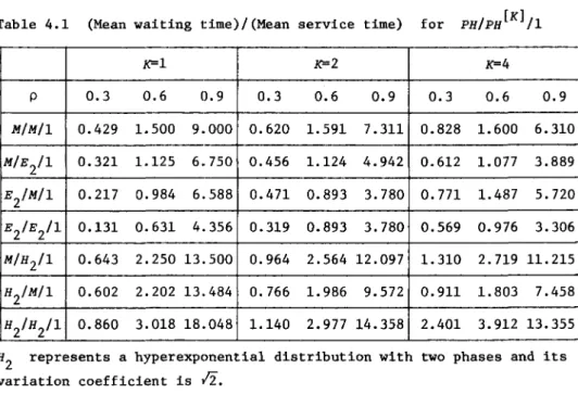
Table 4.1 and Fig. 4.1 demonstrate many interesting results. For exam-ple, in Fig. 4.1, the larger the variation coefficients of the interarrival and the service time distributions, the longer the mean waiting time. It is also found that, in the light traffic case, the larger the service batch size, the longer the mean waiting time, but, in the heavy traffic case, the larger the service batch size, the shorter the mean waiting time, if the interarrival time distribution, the service time distribution, and the traf-fic intensity p are fixed. In Fig. 4.2, it is found that the waiting probability depends on the service batch size. However, in the light traffic case, the larger the variation coefficients of the interarrival time distri-bution and the service time distridistri-bution, the larger the waiting probability, but, in the heavy traffic case, the larger the variation coefficients of the interarrival time distribution and the service time distribution, the smaller the waiting probability, if the service batch size is fixed and only when

K 2:, 2.

Table 4.1 (Mean waiting time)/(Mean service time) for PH/PH[K]/l

1\-1 1(=2 1(=4 P 0.3 0.6 0.9 0.3 0.6 0.9 0.3 0.6 0.9 M/M/I 0.429 1.500 9.000 0.620 1.591 7.311 0.828 1.600 6.310 M/E 2/l 0.321 1.125 6.750 0.456 1.124 4.942 0.612 1.077 3.889 EzlM/l 0.217 0.984 6.588 0.471 0.893 3.780 0.771 1.487 5.720 EzlEzll 0.131 0.631 4.356 0.319 0.893 3.780 0.569 0.976 3.306 M/H 2/l 0.643 2.250 13.500 0.964 2.564 12.097 1.310 2.719 11.215 HzlM/l 0.602 2.202 13.484 0.766 1. 986 9.572 0.911 1.803 7.458 HzlHzll 0.860 3.018 18.048 1.140 2.977 14.358 2.401 3.912 13.355

H2 represents a hyperexponential distribution with two phases and its variation coefficient is

12.

PH/PH/l with Batch A"ivais or Services 29

Fig. 4.1 (Mean witing time)/(Mean service time) for PH/PH[K]/l

Fig 4.2 20

"/

III //1 10 1/' I I I 8 _{/ / /} 6 I I I 1/ / 1/ / 4 _;.Y

i /

",'" 2 / /

,J?

/ /'/ / / / / / / / / / / / 1 / / K=tv / I 0.8 / /~=r K=l 0.6 / / / I / / I I I 0.4 ( / I I I / I ( / I I I 0.2 I I I E /E [K] /1 '1I 2 2 1// _, -H /-H [K]/l Ifl 2 2 0.1 I I _{(C 2=c .2=2)} 0.08 III a 5 U I 0.06 0 0.2 0.4 0.6 0.8 1.0 p

The waiting probability of an arbitrary customer for

1.0 0.8 0·6 0.4 0.2 0.0 o 0.2 0.4 . - - - - E lE [K]/l 2 2 - _. - - - H IH [K] /l 2 2 (C a 2_=c s 2.2) 0.6 0.8 1.0 PH/PH[K]/l

30 Y.~ba

Acknowledgements

I wish to express to my deep appreciation to Professor Hidenori Morimura for his helpful suggestions and criticisms. I am also grateful to the

referees for their valuable comments on this paper.

References

[1] Bailey, N. T. J.: On Queueing Processes with Bulk Service. Journal of

Royal Statistical Society, Series B, Vo1.16 (1954), 80-87.

[2] Be11man, R.: Introduction to Matrix Analysis. MacGraw-Hi11, New York, 1960.

[3] Cin1ar, E.: Markov Renewal Theory. Advanced Applied Probability, Vo1.1 (1969), 123-187.

[4] Hunter, J. J.: On the Moments of Markov Renewal Processes. Advanced Applied Probability, Vo1.1 (1969), 188-210.

[5] Lucantoni, D.: Numerical Methods for a Class of Markov Chains Arising in Queueing Theory. M.S. Thesis, Department of Statistics and Computing Sciences, University of Delaware, 1978.

[6] Neuts, M. F.: Probability Distribution of Phase Type. In Liber Amicorum Professor Emeritus H. Florin, Department of Mathematics, University of Louvain, 1975, 173-206.

[7] Neuts, M. F.: Moment Formulas for the Markov Renewal Branching Process-es. Advanced Applied Probability, Vo1.8 (1976), 690-711.

[8] Neuts, M. F.: Renewal Processes of Phase Type. Naval Research Logistics Quarterly, Vo1.25 (1978), 445-454.

[9] Neuts, M. F.: Markov Chains with Applications in Queueing Theory, Which Have a Matrix-Geometric Invariant Vector. Advanced Applied Probability,

Vo1.10 (1978), 185-212.

[10] Neuts, M. F.: Queues Solvable without Rouche's Theorem. Operations Research, Vol. 27 (1979), 767-781.

[11] Neuts, M. F.: Some Algorithms for Queues with Group Arrivals or Group Services. Proceedings of lOth Annual Pittsburgh Conference. Modeling and Simulation, Vo1.10, pt.2 (1979), 311-314.

[12] Neuts, M. F.: Matrix-Geometric Solutions in Stochastic Models - An Algorithmic Approach. Johns Hopkins University Press, 1981.

[13] Ramaswami, V.: N/G/1 Queue and Its Detailed Analysis. Advanced Applied Probability, Vo1.17 (1980), 222-261.

PH/PH/l with Batch Arrivals or Services

Press, 1962.

[15] Takahashi, Y. and Takami, Y.: A nwnerical Method for the Steady State Probabilities of a GI/G/c Queueing System in a General Class. Journal

of Operations Research Society of .Japan, Vol.19 (1976), 147-157.

Yutaka BABA: Department of Information Sciences, Faculty of Science, Tokyo Institute of Technology, Oh-okayama, Meguro-ku, Tok}'O 152, Japan.