Piecewise Linear Dynamic Programs with Applications

Society of Japan

Vol. 23, No. 2 .. June 1980

Abstract

PIECEWISE LINEAR DYNAMIC PROGRAMS

WITH APPLICATIONS

Katsushige Sawaki Nanzan University

(Received May 22, 1978; Revised May 11, 1979)

This paper considers a special class of dynamic programs which satisfies the monotone and contraction assumptions. This class of dynamic programs is charaC1:erized by the piecewise linearity that the cost function is piecewise linear whenever the terminal cost function is pi'~cewise linear. Partially observable Markov decision processes have this property.

An algorithm based on policy improvement is develo ped to construct f·optimal policies and f-optimal cost func-tions. This algorithm has the advantage of involving only linear funcfunc-tions. A numerical example is also presented.

1. Introduction

Blackwell [1], Denardo [4], Straueh [14] et al consider a general class of monotone eontractive dynamic programs. In this paper we consider a special class of Denardo' s dynamic programs which satisfies the monotone and contraction assumptions. This class of dynamic programs, called piecewise linear dynamic programs, has the property that only piecewise linear cos t functions and piecewise constant policies are involved. A partially observ-able Markov decision process ([6],[11],[12],[13]) has this property.

Larson [9] develops a theory, as "IITell as an algorithm, for a state Incre-ment dynamic programming which is appU.ed to the continuous time model where

the state dynamics is described by differential equations. The concept of "state increment" is similar to the one of simple partition in this paper in the sense that a convex polyhedral cell of a simple partition corresponds to

essentially finite-state d~~amic programs to approximate denumerab1e state dynamic programs. B1ackwe1l [1] and Strauch [14] also introduce the concept of essentially finiteness of the action space to approximate uncountable (Polish) state dynamic programs, but they neither mention how to cons tract an optimal policy and optimal cost, nor provide an algorithm. In this paper we show how to generate and construct E-optima1 costs and E-optima1 policies over simple partitions of which cells are convex polyhedrons. Furthermore, an algorithm is provided. It includes policy improvement and successive approxi-mation as special cases. Its advantage is that we only have to involve linear equa1ities and linear inequalities.

In Section 2 piecewise linear dynamic programs with an abstract state space and finite action set. over an infinite horizon will be discussed. Section 3 will introduce se.vera1 examples having piecewise linearity. Model 1 is actually a basic mathe,matica1 model which includes Model 2, a partially observable Markov decision process as a special case. Model 3 is a machine maintenance model under uneertainty. Model 4 is rather a dynamic economic linear model. Section 4 explicitly develops the algorithm based on a modified policy improvemen t and a proof f or the convergence. Sec tion 5 provides a numerical example and concluding remarks.

2. Piecewise Linear Dynamic Programs

First, we shall formulate a general dynamic programming problem under the setting of Denardo [4]. Secondly, a piecewise linear dynamic program will be defined. It is a special class of general dynamic programs which satisfies the mono tonici ty and contrac tion assumptions.

The state space Si is an arbitrary set of a real linear space. For each x E Si there is a set Ax of actions. Let ~ be the Cartesian product x~SiAx' An element 6 E ~ is a policy. There is always an optimal stationary policy among

a general class of policies in a contractive monotone dynamic program by Denardo [4] or Blackwell [1]. It suffices to consider only the class of stationary policies. Let V be the set of all bounded real valued functions on Q. An element of V is a cost function. V is a Banach space with the norm

Ilvll = suplv(x) I. For u, v £ V we write u ~ v if u(x) ~ v(x) for all x £ Q. x£Q

The loss function h is defined to be a mapping from u {x} x A

x£Q x x V to a real number. Our objective function to be minimized is somehow ambiguous, unless that the loss function h is specified. In a Markov decision process, hClwever, h(x,a,v) can be written as h(x,a,v) = c(x,a)

+

SfQv(y)q(dylx,a) where c(x,a) is the immediate cost, S the discount factor and q(olx,a) the transition probability on Q given x and a. Therefore, note that the system dynamics as well as the objective function is conc,ealed behind our formulation. Assume

that the loss function satisfies the monotonicity and contraction assumptions, that is, for each x £ Q and a £ A h(x,a,u) ~ h(x,a,v) whenever u ~ v in V,

x

and for some S£[O,l), Ih(x,a,u) - h(x,a,v) I ~

si

lu-vl I for each u,v £ V,x £ Q and a £ Ax' For

0

£ ~ define U

o : V ~ V by (Uov)(x) = h(x,o(x),v) for v £ V and x £ Q. Assume that there is some

;5

£ ~ such that U v = inf U v. Also,

8"

o£~ 0 define U*: V ~ V by U*v = inf U v. If o(x)

oe:6 0

a for each x e: n, then we write U = U Denardo [4] verifies that U* and U are monotone contraction

opera-a

o'

0

tors. By Banch's fixed point theorem, for each

0

£

~

there is a unique vo£V

o

0

*

*

such that Uov = v. Similarly there :ls v £ V such that U*v v . Such v

*

0

*

and v are called the cost of the poliey 0 and the optimal cost, respectively.

*

0 0

*

Denardo [4] shows that v = inf v I f Ilv - v II

:s.

£, then 0 is an £-optimal

*

o£~

policy, and if I Iv-v I I

:s.

£, then v is an £-optimal cost function. Our purpose is to find such £-optimal policy and £"optimal cost function.

Any set of the form {xe:n : £ij(x) < (or ~) d

j,j=1,2, ... ,ni},i=1,2, ... ,m, where £i' is a linear func tional and d

l

, a real number is called a convex

J .

polyhedron. A collection P = {E

m is the number of cells in the partition. If each cell of a partition is a convex polyhedron, then the partition is called simple. The product of two

1 d 2 p1. 2 {

partitions

P

an

P

is .p '" EnD: E € P , 1 D €

p}.

2 The product of

~.p2

...

pn

is defined inductively by

m m-1

IT pi =

pn.

IT pi. Plainly, the finite

i=l i=l

product of simple partitions is again simple. A vector valued function v on Q is piecewise linear (abbreviated, hereafter, by p.w.) if there exists a simple partition {E

l,E2, .•. ,EJOf

n

and m linear functions vl,v2, ..• ,vm such that v(x) = vi(x) for all x € E

i, i=l,2, ... ,m. A policy 0 is piecewise (p.w.) constant if there is a simple partition {E

l,E2, •.. ,Em} of n and m actions al, a

2, ... ,am, such that 6(x) = ai for all x € Ei, i=l,2, .•. ,m. A p.w. constant policy is simple and easily represented in a computer. For example, a bang bang control is such p.w. constant policy. The paper Denardo and Rothblum [5] discusses affine (but not piecewise) dynamic programs.

*

*

Although v is not necessarily p.w. linear and 0 is not necessarily p.w. constant, we will show for a class of dynamic programs having the structure described in the following assumption that there are €-optimal p.w. linear cost functions and p.w. constant policies.

Assumption I (A.I.).

For each a, (U v) (x) is p.w. linear on Q, provided that a

v is p.w. linear on Q.

The following theorem shows that the structure in Assumption I implies how U* and U

6 preserve the p.w. linearity of loss functions and the p.w. constant of policies. Assume from now on that Ax = A = {a

l,a2, •.• ,ap} for all x € Q is finite.

Theorem

1. Suppose that (A.I.) holds and that v is p.w. linear. Then (i) Uov is p.w. linear whenever 6 is p.w. constant;

(ii) _{U*v is p.w. linear; and}

(iii) there exists a p.w. constant policy 0 such that U

Proof·

(i) Suppose that a is p.w. constant with respect to a simple partition

(H)& (Hi)

{E

i}. Let Ei be an arbitrary but fixed cell from the partition and suppose that a(x) = a for x t: El. Then

(u v) (x)

a for

From (A.I.), Uav is p.w. linear for each a. Hence Uav is p.w. linear on eaeh cell E

i, and is consequently p.w. linear on rl.

The functions U v are each p.w. linear by (A.I.). Suppose that U v is

a a

p.w. linear with respect to the simple partition pa. Let P = IT p.a. ae:A Then

P

is finer than each pa, and so each U v is p.w. linear with

a

respe<:t to P. For each F e: P and a e: A, there is some linear funl:-a

tional CIF such that

(U v) (x)

a for X t: F.

b For each F t: P, define the sets G

F, b t: A

=

{1,2, ... ,p}, by Gb={· F .x: aFx b < aFx, a=l,2, ••. ,b-l and aFx a b S a~, a a=b+l, ..• ,p . }

Then {G; : a t: A} =

PF

is a partition of F and P = IT

PF

is a partition Ft:P

of rl with the property that

a

~(x) i f

The policy a defined by a(x) a for X ~ _~ Ga _F c _~ P _{sa s} ti fi _{es a}U V U ... v.

Corollary.

Suppose that (A. I.) holds and that v

o

t: V is p.w. linear. (i) (Uav n-1 )(x), n=1,2, ... , for p.w. constant a.

(ii) Define v (x) = (U*v n n-1 )(x), n=1,2, ...

Then vn is p.w. linear and there exists a p.w. constant stationary n-1

policy, on' satisfying U o v

n

We next consider the effects of iterating monotone contraction mappings such as U* and Uo' citing some results of Denardo [4].

Lemma

1. Suppose that U is a contraction mapping on V with contraction coef-ficient S < 1. Let vO E V be given and define the functions vn, n=1,2, ... by

n-1 (Uv ) (x) •

Then

'(i) {vn} converges in norm to the fixed point "-v of U; i.e. , Uv v. Now assume that U is also monotone.

(ii) If v 1 ,;:: v 0

,

then {vn} is mono tonically decreasing to ~. (iii) If v 1 ~ v , 0 then {vn} is mono tonically increasing to v.

Remark.

The fixed point

v

need not to be p.w. linear since the cells in the limiting partition are not necessarily finite in number nor polyhedral.

3. Examples

Model

1.

A Markov decision process

(B1ackwe11 [1])

Let

n

be a bounded convex polyhedron in RN and the loss function

h(x,a,v) c(x,a)

+

Sfnv(x')q(dx' Ix,a) as mentioned in the preceding section. Assume that c(x,a) = ca.x, which may be interpreted to be the expectation of ca if x is a probability vector. Also assume that for each convex polyhedron

is p.w. linear in x with respect to a simple partition

{E. (a,B), j=1,2, •.. ,m B} for each a where the integral of the vector

J a,

x' is defined componentwise. These two assumptions imply

(A.I.).

We explicitly check that

(A.I.)

is satisfied. Let a €

A

be arbitrary but fixed and suppose that v is p.w. linear with respect to a simple partiti.on

m {E

i, i=1,2, ... ,m}. Let pa = _i=l IT pa(E.)

1.

{-a E }

j ; j=1,2, ... ,r , the product partition, which is again simple.

(U v) (x) a ca " x

+

Sfnv(x')q(dx' Ix,a) m ca " x

+

S

E

lE

(vix')q(dx'lx,a) i=l i m

cax

+

S E v. " (lE x'q(dx' Ix,a)) i=l 1. i m ca " x

+

S

E

V.qa(E.,X) i=l 1. 1. m [ca

+

Q 'C \ a ] IJ t.. vil\ .. x i=l 1.J for X E: E.(a,E.) J 1. a a

where Aij"X = q (Ei,x) for x E: Ej(a,E

i) and the index j depends on i for each a E: A. The third equality is obtained from the fact that the integral of the inner product is equal to the inner product of the integral if vi does not depend on x, a and each componentwise integral is well defined. U v is linear

a

on each E:~. Hence U v is p.w. linear 'with respect to the simple partit:i.on

J a

pa={E~,j=1,2, ... ,r}, which satisfies (~.I.). J

Model 2. A partially observable Markov Decision Process (Sawaki and Ichikawa [11], Dynkin

[6])

We will show that a partially observable Markov decision process, model 2, is a special case of model 1. Consider a Markov decision process with state space {1,2, ..• ,N}, with fini.te action set A, with probability transition matrices pa and with immediate cost vectors ca. Let Z be the state at the n-th transition.

n

Assume that the process {Z , n=O,1,2, .•.. } cannot be observed, but at each tran-n

sition a signal 8 is transmitted to the decision maker. The set of possible signals e is assumed to be finite. For each n, given that Zn = j and that action a is to be implemented, the signal en is independent of the history of the signals and actions {eO,aO,e1,a1, .•• ,8n_1,an_1} prior to the n-th transition and has conditional probability denoted by Y~8 =

p[e

=81z =j,a l=a].

J n n

n-N N

Let ~ = {X=(X

1,x2' ... ,xN): i~lxi=l'Xi~O,Vi}CR. Define the i-th component of X

n, the random variable of x, to be

P[Z n

It can be shown (see Dynkin [6]) that

j 18 +1' a ,X ]. _{n n n}

Thus Xn represents a sufficient statistics for the complete past history It follows that {X : n=O,1,2, ... } is a Markov

n

process (see Dynkin [6]), called the observed process. Its immediate cost is c(x,a) = ca • x. Its probability transition function is determined by the following calculation. For each measurable subset B ~~, X E ~, and a E A,

q(Blx,a) a = a] n S IZ n+1 j, Xn

=

x,a] • P[Zn+l

LP[X 1

E: Bls n+1 S, X = x, S n+ n a n j Ix

=

x, a

=

a] n n a]

.

L

a EP[Z +1 j Y jS i n j Iz _n = i, X _n = x, a _n a]P[Z = ilx = x, a = a] n n n ~P[Xn+1 E: B I Sn+l ~P[Xn+1 E: B le n+ 1

where 1:. (1,1, ... ,1) and pa(S) T(xIS,a) by

T(x

I

S ,a)

Note that T(X IS,a)

n Xn+1' and that S, X n e, X n P[Xn+l E: Bls_n+₁ e,x _n

=

x, a _n

=

a] So,

=

x, a _n

=

_{a]Eyos l.PijXi} a a j J _i x, a _n a] 1:.pa(S)x i f T(xIS,a) E: B if T(xIS,a) ~ B.

where ~a(b,x)

=

{6: T(xI6,a) E B}.

Finally, we show that the observed process {X lis a special case of Model n

1;

i.e., qa(B,x)

=

fBx'q(dx' Ix,a) is p.w. linear in x for each convex poly-hedral set B c ~ and action a EA. Using the previously computed q(Blx,a) we have

L

T[xI6,a]! pa(6)x

13E~a(B,x)

L pa(6)x

i1da(B,x)

which can be shown to be p .1 •• linear (see Brumelle and Sawaki [2]).

Model 3. A Machine Replacement Model with Partially Observable States

This model is an applieation of partially observable models into the quality control model modified from Sawaki and Ichikawa

[11].

A machine consists of n internal components. The state of the machine is the number of working components. The machine produces constant finished products

(say M units) and the machine cannot be inspected, that is, the state of the machine is unobservable. Let 6 be the number of defective products out of M finished products. ASSumE! that the conditional probabilities of finding 6 given the machine in state i are given by

when the machine is not replaced. Assume that Y

OO

=

1 and Yoe

=

0 for e > 1. Thus, the only available information about the state is the posterior proba-bi1ity xi and e. I f the probability at: time t is x

=

(x

O"" ,xn) and e has been observed, then i t will be T(xle) ~;iven in Model 2. Let c

i be the operat-ing cost if the machine is in state i and let c

=

(cO"" ,c

n). The rep1.3.cement cost is R > () and the daily expected operating cost is

which is linl~ar in x. It is shown from B1ackwe1l [1] that the minimal expected

*

total discounted cost V (x) is the unique solution to the optimal equation

*

V (x) min {ex

+

Sl:.!.P_y V (T(xle»

*

e e

R

+

SV

*

(eP)}.

Model 4. A C1lassical linear econorrric model

Let x be a price vector of N commodities (or N securities) in the market and assume that a new price vector x' ean be written as

x'

where Q~ is an N x N matrix depending <:m the present economic situation e and on an economic alternative a. Let p[elx,a] be the conditional probabi1i.ty of e forecasted, given x and a. Assume that there exists a simple partition {E

i} of the set of price vectors x such that

p[e Ix,a] for X E: E.,

the class of model 1, provided the immediate cost is well defined.

4. Algorithm and Its Convergence

If the state space

n

is uncountable, or even countably infinite, then the dynamic program is difficult to implement on a computer. However, if the

n dynamic program has the structure of (A.I.) and v is p.w. linear, then U

6v is p.w. linear and each 6n constructed as in Theorem l(11i) is p.w. constant. In

this case, the cost functions and policies can be specified by a finite number of items - the inequalities describing each cell of a simple partition and the corresponding action or linear function.

In this section, we discuss the algorithm in general terms, choosing the 6

parameters {k } which specify the degree of approximation of v in the n-th n

iteration, terminating the algorithm, and a proof that the algorithm converges. The algorithm includes policy improvement and successive approximation as special cases.

A

"igorithm

Start with a simple policy 60 and a p.w. linear function yO

~

V satisfying

o

0

y ~ U oy . 6

An iteration of the algorithm is described as follows: n=0,1,2, . . . . At the start of the n-th iteration, we have a simple policy 6n and a p.w. linear

n . n n

function y E V sat1sfying y ~ _{U nY}

6

S

is a contraction operator's coeffi-cient.

(i)

(11)

k

Compute U nyn where the integer k

6n n is the number of iterations of U ₆n which are to be performed.

n+1 Set y

k

n n n+1 n+1

U nY and find a policy 6 such that U n+1Y

(Hi) _{If Ily n _ yn+lll 5 (1 -S)E, then stop wity yE-optimal and} n J:: u n E-optima1.

*

on n+1

:s

v .::: y Moreover, v If Ilyn - yn+111 > (1 - Q)~,

(iv) fJ c. then increment n by 1 and perform another

iterat.ion.

To start., the algorithm needs a simple policy 0 and a p.w. linear function y satisfying y ~ UoY' There is no difficulty in finding a simple policy; for

o

example, o(x) = a for all x €

n

is satisfactory and one can choose y (x) = 0

o

0

for each x E

n

which satisfies y 2! UoY in a Markov decision process with c(x,o)

s

O. Note that if each k _n 1 in step (i), the algorithm is successive approximation and that if each k

n 00, the algorithm is reduced into policy improvement.

Theorem 2. For each iteration, n=0,1,2:, ... , in the algorithm,

k _ > U nyn n

o

n+l y

In other wards, {yn} is a decreasing sequence.

By definition

0

1

O. Since Y 0 ~ U ay and since U0 oO 0 _{> U}

₀

_> 2

0 0

kO 0 y - ay - U ay ~ ..• 2! U ay

0

₁

0

₁

₀

satisfies U cS y = U*y . However,

Proof. First, it is true for n =

monotone, it follows that

is 1 ~ = y U*y 1 5 1

< y1, and so not only is the Theorem established for n = 0, but

h 1 h h U 1 , 1

we ave a so s own t at 1Y :: y

o

Now suppose U yn 5 yn. The same argument as in the first paragraph on

establishes the Theorem for n and also that U yn+1 < yn+1 Hence

on+1

-the proof is completed by induc: tion .

Proof· For an arbitrary n, y n ~ U nY n ~ U*y n Since U* is monotone, y n ~

o

u~yn

for each j. By Lemma 1, utyn decreases mono tonically

~: n

*

and converges to v as j + 00. Consequently, y ~ v and the proof is

complete.

We next show that if the algorithm terminates then it will provide an €-optimal cost function and an €-optimal policy.

Theorem 3. I f [[yn - yn+l[[ S (1 - S)€, then [[yn _ v*[[ S €, Le., yn is

*

0

€-optirnal. Moreover, On is also €-optimal and v ~ v n ~ yn.

Proof· Note that U nyn

o

n n

*

u*y and that by the previous corollary y ~ v .

Ilyn_umynll Iln *11

<

+

S y - v for m=1,2, .•. ,

on

because _Yn _> U yn _on _> Urn _on yn _{for m = 1,2, . . . . (Theorem 2.)}

Thus

and so

The last statement in the Theorem follows by Theorem 2 and Corollary.

Theorem 4. Suppose that {yn} is a sequence of costs generated by the algorithm.

(i) yn converges pointwise to y €

v.

(11) y = U*y, Le., y is optimal. In other words, the algorithm converges.

Proof·

(i) First of all we shall show that {yn} is bounded below. By Theorem 2 we have yn :2: Urn yn for each m

=

n m

&

on

[4])

that U y ~ v

on as m

~ "".

1,2, ... It is well known (see [1] and

n on on *

Therefore y :2: v . From v ~ v € V, 6_n

there exists an M such that Ilv

11::;

M. Hence yn(x)

?

-M for all x. From Theorem 2 yn is a decreasing sequence. Hence yn converges point-wise.

(ii) B y a C h · 01ce of yO an d Th eorem 2 we k now t at h

(2)

To show the other way we have

n y _U m _n-1Y n-1

o

n-1

:::; u

n-1Y

o

Then, from (1) and (2), we obtain

(By definition of yn)

m

(Uoy ~ Uy, ¥y € V)

n-1 (By definition of 0 ) .

From the statement (i) yn ~ y. Since a contraction mapping U* is continuous, n

5. A Numerical Example and Conclusion

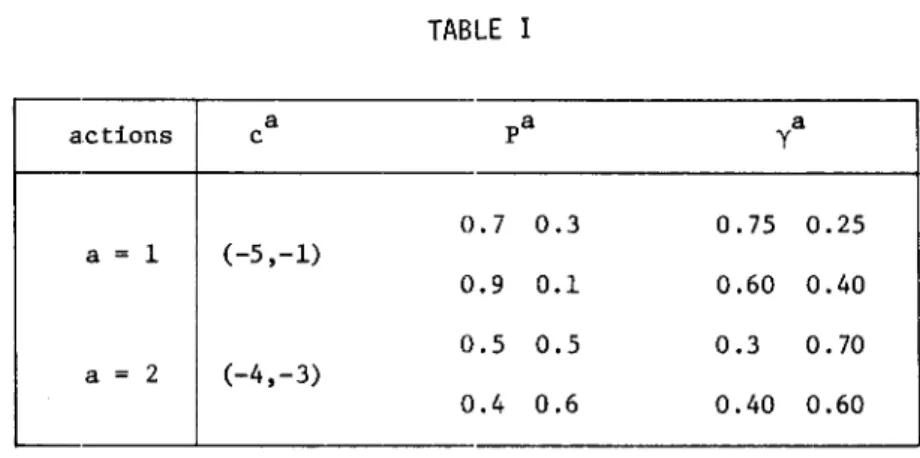
This section presents a numerical example for Model 2, partially observa-ble Markov decision processes, especially in the case of two demensions,

{l,2}. The necessary data are shown in Table I. To specify the stopping rule we choose

iiyn _ yn-lii ~

S

= 0.8 and s = 0.01. Therefore, if 0.002, then the algorithm stops and yn is s-optimal.

Set xl = x. To start the algorithm an initial p.w. constant policy 0 and

°

°

an initial p.w. linear cost function y satisfying yO ~ U

°

oOY must be found. Choose a policy 0° minimizing ca,x; thus oO(x) = 1 if x

~

2/3, oO(x) = 2 if x >

2/3. Set an initial cost function yO(x) =

(O,O)[l~x]

with the partition {[O,l]}, which is p.w. linear and satisfies yO

~

H oyO. Also set k = 1 for

o

n

all n. The computational results programmed in FORTRAN are shown in Table 11. We may observe from Table 11 that the algorithm converges at period n=35, and an s-optimal cost is -15.l66-3.826x if x ~ 0.571 and -16.732-l.086x if x >

0.571. An s-optimal policy 030(x) = 1 if x

~

0.571 and 030(x) = 2 if x > 0.571. Table 11 also shows that an s-optimal policy converges (at n=lO) much faster than an s-optimal cost does.

The goal of this paper is to generate and construct s-optimal costs and s-optimal policies in a sequential fashion for a general class of dynamic programs. Toward this end we have taken advantage of the properties of p.w. linear cost functions and p.w. constant policies. These properties guarantee that the algorithm involves only p.w. linear and constant functions which belong to the class of linear programs. Finally we should also emphasis the importance of the algorithm capable for solving continuous state dynamic programs. Many sequential decision problems under uncertainty often turn out to have a probability vector as their state space, which is no longer finite nor countably infinite, but continuous. Therefore, the algorithm developed

in this paper will become more important in the field of sequential decision problems under uncertainty.

TABLE I actions c a pa y a 0.7 0.3 0.75 0.25 a

=

1 (-5,-1) 0.9 0.1 0.60 0.40 0.5 0.5 0.3 0.70 a

=

2 (-4,-3) 0.4 0.6 0.40 0.60 TABLE II

Periods n cost functions y n Policies and Partitions \\yn_ yn-.1\\

1 -1-4x 1 [0.00,0.666] 5.00 -3-x 2 (0.666,1.00] 2 -4.12-3.84x 1 [0.00,0.579] 2.96 -5.719-1.08x 2 (0.579,1.00] 3 -6.35-3.827x 1 [0.00,0.572] 2.22 -7.92-1.086x 2 (0.572,1.00] 5 -9.53-3.826x 1 [0.00,0.571] 1.411 -11.095-1.086x 2 (0.571,1.00] 10 -13.324-3.826x 1 [0.00,0.571] 0.462 -14.889-1.086x 2 (0.571,1.00] 20 -14.975-3.826x 1 [0.00,0.571] 0.05 -16.540-1.086x 2 (0.571,1.00] 30 -15.152-3.826x 1 [0. 00,0. 571] 0.005 -16. 717-1.086x 2 (0.571,1.00] 35 -15.166-3.826x 1 [0.00,0.571] 0.001 -16.732-1.086x 2 (0.571,1. 00]

Acknowledgement

The author would like to express his thanks to the referees for their helpful comments and suggestions. Thanks also to Dr. Seiichi Iwamoto for informing him the references [7] and [9]. The author is also grateful to Professor Y. Iihara for his suggestions and encouragement.

This research was part.ially supported by the Nanzan University Research Grant A (1979).

References

[1] Blackwell, D.: Discounted Dynamic Programming,.

Annals of Mathematical

Statistics,

36(1965), 226-235.

[2] Brumelle, S.L. and Saw.aki, K.: Generalized Policy Improvement for Simple Dynamic Programs, Working Paper 546, Faculty of Commerce, University of British Columbia, Vancouver (1978).

[3] Brumelle, S.L. and Puterman, M.L.: On the Convergence of Newton's Method for Operators with Supports, University of California, Berkeley (1976). [4] Denardo, E.V.: Contraction Mappings in the Theory Underlying Dynamic

Prograrrming,

SIAM Review

9 (1967), 165-177.

[5] Denardo, E.V. and Rothblum, U.G.: Affine Dynamic Programming, Proceedings of the International Conference on Dynamic Programming and Its

Applications, University of British Columbia (1977):

Dynamic Programming

and Its Applications

(ed. M.L. Puterman), Academic Press (1978), 255-267. [6] Dynkin, E.B.: Controlled Random Sequences,

Theory of Probability and Its

Applications

X(1965), 1-14.

[7] Fox, B.L.: Finite-Stat,= Approximations to Denumerable-State Dynamic Programs,

Journal of M~thematical Analysis and Applications, 34(1971),

[8] Howard, R.A.: Dynamic Programming and Markov Processes, Wiley, New York (1960).

[9] Larson, R.E.: State Increment Dynamic Programming, Elsevier, New York (1968) .

[10] Sawaki, K.: Piecewise Linear Markov Decision Processes with An Applica-tion into Partially Observable Models, presented at the 1978 InternaApplica-tional Conference on Markov Decision Pro.:esses, University of Manchester (1978). [11] Sawaki, K. and Ichikawa, A.: Optimal Control for Partially Observable

Markov Decision Processes Over an Infinite Horizon, Journal of Ope1>ations

Research Society of Japan, 21(1978). 1-16.

[12] SmallwClod, R.D. and Sondik, E.J.: The Optimal Control of Partially Observable Markov Processes over a Finite Horizon, Operations Research,

21(1973),1071-1088.

[13] Sondik, E.J.: The Optimal Control of Partially Observable Markov Processes over the Infinite Horizon: Discounted Costs, Operations

Research, 26(1978), 282-304.

[14] Strauch, R.E.: Negative Dynamic Programming, Annals of Mathematicai:

Statistics, 37(1966), 871-890.

Katsushige SAWAKI: Faculty of Business Administration, Nanzan University, 18, Yamazato-cho, Showa-ku Nagoya, 466 Japan