On Dual Differentiable Exact Penalty Function for Equality Constrained Optimization

Journal of the Operations Research Society of Japan

Vol. 28, No. 4, December 1985

ON DUAL DIFFERENTIABLE EXACT PENALTY

FUNCTIONS FOR

Abstract

EQUALITY CONSTRAINED OPTIMIZATION

Masao Fukushima Kyoto University Hisashi Mine Kansai University Eiki Yamakawa Kyoto University

(Received November 12, 1984: Revised June 12, 1985)

This paper is concerned with a differentiable exact penalty function derived by modifying the Wolfe dual of an equality constrained problem. It may be considered that this penalty function belongs to a class of general augmented Lagrangians on which other differentiable exact penalty functions are based. It is shown that this penalty function possesses an attractive property which may be enable us to use Newton like method effectively, Some numerical results are also reported.

1. Introduction

Much attention has been paid on differentiable exact penalty functions in constrained optimization [1,2,3,4,5,7,17]. In general, such penalty functions are constructed by performing some modification to augmented Lagrangians. Recently, Han and Mangasarian [12] have introduced a class of differentiable exact penalty functions by using the Wolfe dual of inequality constrained problems. Differentiable exact penalty functions are quite attractive from a computational viewpoint, though their expressions are somewhat involved. In fact, they overcome somE' disadvantages of nonsmooth exact penalty functions [11,16] when used in connection with sequential quadratic programming methods [9] .

In this paper, WE' consider dual exact penalty functions of Han-Mangasarian type for equality constrained problems. We explicitly state conditions under which a Karush-Kuhn-Tucker CKKT) pair of the original problem © 1985 The Operations Research Society of Japan

affords an isolated local maximum of the dual exact penalty function. Also, we show that this exact penalty function and those considered in [1,2,3,4,17] belong to the same class of general augmented Lagrangians containing parame-ters. That j.s, we point out that a KKT pair may actually correspond to a local minimum [1,2,4], a saddle point [3,17] or a local maximum of the general augmented Lagrangian according to the manner in which the parameters are chosen. In addition, we mention that, in a neighborhood of a solution, we can conveniently approximate Newton directions for unconstrained maximization of the dual exact penalty function by those for solving Karush-Kuhn-Tucker equations.

2.

Local Duality Results

We consider the following equality constrained problem minimize

f(x)

(1)

subject to h(x)

=

0 ,

where f :

JIl

+ RI , h : Rn + Ef1 , and m < n We assume that f and harE

twice continuously differentiable on

JIl

The Lagrangian L : JIl+m + RI for problem (1) is defined by

L(x,U)

=

f(x)

+

uTh(x) ,

where U is the vector of Lagrange multipliers. The gradient and the Hessian of

L

with respect to x and U are given by

\7L(x,U) [ \7x L

(x,U)

1

[ \7xL(x,u) \7 L(x,U) h(x)

u

[ \72 L(x,U) \7~uL(x,u)

₁

_{= [}

\7~xL(x,u)

\7h~X)

1 '

\72L(x,U) xx

'12 L(x,u) _\7~uL(x"u) \7h(x)T UX

respectively, where \7h(x) denotes the n x m matrix whose columns are the gradients If x* is a local solution of (1) , then, under a regularity assumption, there exist multipliers U* such that (x*,U*) satisfies the first order optimality conditions [6,8] :

(2) IJL(x,u)

o .

Equations (2) are refered to as Karush-Kuhn-Tucker (KKT) conditions • Also, x* and (x*,U*) are called a KKT point and a KKT pair of (1), respectively. In the subsequent arguments, we shall often give attention to KKT pairs

304 M Fukushima, E. Yamakawa and H. Mine satisfying the second order sufficient conditions [6,8]

(3)

/V~xL(X*

,]1*)Y

> 0 , 0 '" 'ify E { y

I

Vh(x*)Ty

=

0 , Y E

If1 }

and the regulari t y condi tion :

(4)

V\

_(x*),

i l, ..• ,m , are linearly independent.

For problem (1), we can formally define the Wolfe dual [10,14] as follows: maximize

L(x,]1)

(5)

subject to V

L(x,]1)

x

o .

It is well known that, if f is convex and h is affine, then global duality holds for problems (1) and (5) [14, Chapter 8].

Han and Mangasarian [10] have recently established results: For a KKT pair

(x*,]1*)

of (1), if definite on the subspace spanned by

Vhi(x*)

satisfies the second order sufficient conditions

For general cases, Fujiwara, the following local duality

2 -1

is positive V

L(x* ]1*)

xx '

i

= 1, .•. ,m

,

then

(x*,]1*)

for the dual problem (5) [10, Theorem 2.2]. In general, however, this assumption does not appear to be fulfilled for nonconvex programming problems, as illustlated in the next example.

Example. Consider the following nonconvex programming problem minimize

_"2

1 ( 2 2)

Xl

-X2

(6)

subject to

h(Xl,X2)

X2

=

0 .

The Lagrangian L for problem (6) is defined by

It is clear that Xl*

=

X2*

=

0 is the unique optimal solution of (6) and ]1* 0 is the corresponding Lagrange multipliers. But we have

In fact, for problem (6), the Wolfe dual is defined by maximize

_"2

1 ( 2 Xl

-X2

2)

+

]1X2

(7)

subject to xl

=

0 ,

-X2

+

]1

=

0 Since problem (7) is equivalent to the problem

maximize

1..

X 2

and its optimal value is

+"" ,

there is a duality gap between problems (6) and

(7).

o

Now we construct a modified Wolfe dual of problem (1), for which the local duality holds under more natural assumptions.

following problem

Let us consider the

minimize

f(x)

+

~

Ilh(x) 112

(8)

subject to

hex)

=

0 ,

where t is a nonnegative parameter. It is obvious that problem (8) is equivalent to problem (1) for any t

.

I f

(x*,\1*)

is a KKT pair of problem (8), then

(x*,\1*)

is also a KKT pair of (1) , and vice versa [13, p.321). The Lagrangian Lt : JIl+m+Rl for problem (8) is given by

Lt (x,\1)

=

f(x)

+

~llh(x)112+

\1Th(x)

=

L(x,\1)

+

~llh(x)112

This function is well known as the augmented Lagrangian [2,3,9,13], which is frequently used as a means of resolving duality gap in nonconvex programming. Then we can write the Wolfe dual for problem (8) as follows:

maximize (9)

Because problem (8) is equivalent to (1), we can regard problem (9) as a dual problem of (1) for any t ~ 0 •

We now proceed to establish local duality results for problems (1) and (9). First of all, we shall begin with the following simple theorem.

Theorem 1. (a) I f

(x*,\1*)

is a KKT pair of

0),

then

(x*,\1*)

is a KKT point of (9). (b) Let

(x*,\1*)

be a KKT point of (9) and assume that

V!xLt(x*,\1*)

is nonsingular. Then

(x*,\1*)

is a KKT pair of (1).

0

The proof of this theorem is similar to that of [12, Theorem 1], and hence is omitted here.

The next local duality theorem will play an important role in validating the dual exact penalty function approach to be developed in the subsequent section.

Theorem 2. Let

(x*,\1*)

is a KKT pair of (1) satisfying the second order sufficient conditions (3) and the regularity condition (4), Then there exists a

t*

~ 0 such that, for any

t

~

t*

(x*,\1*)

is an isolated local maximum of problem (9) and

f(x*)

=

L

306 M. Fukushima. E. Yamakawa and H. Mine

Proof: By Theorem 1 (a), (x*,~*) is a KKT point of

(9).

By (3), it

1,72 L

(x*

~*)

such that, for any t ~

t*

,

_xx

_{t '}

follows that there exists a

t*

~ 0

is positive definite [13, p.321]. Hence I,7xxLt(x*,~*) 2 -1 exists and is also positive definite. Therefore, by (4), we have

w

=

I,7h (x*)z,

0 '" Z E

If1

+ T

2 -1

w

1,7 L

(x*

~*) w > 0 .

xx

t '

This is equivalent to the standard second order sufficient conditions for problem (9) [10, Theorem 2.2]. Thus (x*,~*) is an isolated local maximum of (9) for any

t

~

t*

The last assertion of the theorem follows immediately

from the fact that

h(x*) =

0 •

0

3.

Dual Differentiable Exact Penalty Functions

For the equality constrained problem (1), our penalty function is defined by constructing an exterior penalty function [6] for problem (9) as follows

where y is a positive parameter. The penalty problem is then

(11) maximize e(x,~;t,y), (x,~) E If+m •

Note that Han - Mangasarian penalty function [12] is a special case ( t = 0) of (10). As in [12], we can write the gradient of the penalty function (10) with respect to x and ~ as

Moreover, if (x*,~*) is a KKT pair of (1), then the Hessian of (10), evalu-ated at (x*,~*), may be given as

(13) I,72e(x*,~*;t,y)

[

1,72 L

(x* U*)U - yl,72 L

(Xif ~*)}

xx t

'

n

xx t

'

T

I,7h(x*)

{I

_yl,72 L

(x*

~*)} n xx t ' {I -_n

yl,72

_xx

Lt(x*

,~*)}I,7h(x*)

1

T '

-yl,7h(x*)

I,7h(x*)

where

In

is the unit matrix of dimension

n.

In the subsequent discussion, it will be convenient to rewrite (la), (12) and (13) respectively as follows:

1 T

(14) (15) where

V6(x,].1;t,y)

(I

_n+m

+ -2

1

V2L(x,U)K[x;t,y]

1

+

2

V[K[x;t,y]VL(x,].1)]}VL(x,].1) ,

{In+m

+

V

2

_{L(x;*, ].1*)K[x*;}

_{t, y]}}

_V

2

_L(x*,].1*)

K[x;t,y]

= [

-:In

t~

I -

y [ m

o

T

cVh(x)

tVh(x)

t

2

_Vh(x)T'Vh(x)

I .

Note that these expressions are closely related to those of Bertsekas [1,2], although the definition of matrix

K

is quite different.

The next theorem, which corresponds to [12, Theorem 1], shows the rela-tionship between the first order optimality conditions for problems (1) and (11) •

Theorem

3.

(a) I f

(x*,].1*)

is a KKT pair of (1) , then

V6(x*,].1*;t,y) =0

for any

t

and

y

(b) Let

V6(x*,].1*;t,y) =0

and assume that

y-'O

and 1 Y is not an eigenvalue of

V2 L

(x* ].1*)

xx t

'

Then

(x*,].1*)

is a KKT pair of (1) .

Proof: Part (a) is obvious from (14). it follows from (12) that

Let

V6(x*,].1*;t,y)

=

0 • Then,

Since {I -

yV

2

_L

_(x*

_{].1*)}V L}

_(x*

_].1*)

₌

0, n

xx t '

x t

'

h(x*) -

YVh(x*)TV L

(x*,].1*)

= 0 .

x t

it is easy to prove (b) under the hypothesis of the theorem.

D

In the next theorem, we establish conditions under which a KKT pair of (1) affords an isolated local maximum of the penalty problem (11). This theorem may be considered as an extension of Han - Mangasarian [12, Theorem 2] in which similar results are proved by assuming the positive definiteness of

V2

L(x*

].1*) .

xx

'

Theorem 4. Let

(x*,].1*)

be a KKT pair of (1) satisfying the second order sufficient conditions (3) and the regularity condition (4). Then there exist a

t*

~ 0 and, for each

t

~

t* ,

a scalar

y*(t)

> 0 such that

V26(x*,].1*;t,y)

is negative definite and

(x*,].1*)

is an isolated local maxi-mum of (11) for any

y

>

y*(t) •

308 _{M Fukushima, E. Yamakowa and H Mine}

Proof: By Theorem 3 - (a), ity conditions for problem (11).

(x* ,U*) satisfies the first order optimal-Note that,

V2

L

(x* U*)

under conditions (3) and (4), there exists a t* ~ 0 t ~ t* . Let y*(t) > 0 such that denote xx t ' the minimum

is positive definite for any eigenvalue of V2

Lt(x*,u*) •

xx

Then, we can show in a way similar to [12, Theorem 2] that V2e(x*,U*jt,y) is negative definite for each y > y*(t) This completes the proof.

o

Unfortunately, the converse of Theorem 4 does not necessarily hold as depicted in the following example.

Example. Consider the problem minimize

(16)

It is easy to verify that

Xl2

₊

_{(X2 _1)2}

Xl 2 (Xl + 2) - x2

o .

is a KKT pair which corresponds to a local maximum of (16). However, by Theorem 3 - (a), it satisfies the first order optima1ity conditions for the penalty problem given by (11). Moreover, since

and -6 - 36y

o

o

o

o

(t+2)-y(t+2)2 y(t+2)-1 y(t+2)-1 -y

it can be shown that, for each t > 0 and sufficiently large y

is negative definite. Therefore, for such t and V2e(XI*,X2*,U*jt,y)

y , (XI*,X2*,U*) problem.

(0,0,-2) is an isolated local maximum of the penalty

o

This example shows that indefinite V2

L

(x* U*) may also lead to nega-xx t '

tive definite V2e(x*,U*jt,y) In other words, for any t ~ 0 and suffi-ciently large y , every KKT pair of (1) is a local maximum of e even if it does not correspond to the local minimum of (1). Thus in order to establish the converse of Theorem 4, we need a rather restrictive hypothesis that V2 L

xx t is positive definite at a local maximum of problem (11).

Theorem 5. Let (x*,U*) be a local maximum of (11) and assume that (i)

V

2

_{L (x* 11*)}

(ii) Y >' 0 and 1

Y is not an eigenvalue of

V2

xx

L (x*

t ' ]..1*) .

Then x* is an isolated local minimum of (1) with corresponding multipliers ]..1*.

Proof: By Theorem 3 - (b),

(x*,]..1*)

is a KKT pair of (1), so that

h(x*)

=

0 and

V2

L

t

(x*,]..1*)

=

V2

L(x*,]..1*)

+

tVh(x*)Vh(x*)T •

xx xx

Then, it is straightforward to show that the second order sufficient condi-tions (3) for problem Cl) hold under assumption Ci).

o

In summary, any local minimum of problem (1) satisfying the second order sufficient conditions affords an isolated local maximum of the penalty problem (ll) • Conversely, every local maximum of (11) is a KKT pair of

Cl),

but if

V2

L

t

(x*,]..1*)

is not positive definite, x* may not be a local minimum of

xx

(1). This fact appears to delimit the use of the dual differentiable exact penalty functions for nonconvex problems, as compared with the differentiable exact penalty functions such as [1,,2,3,4,5,17] for which sufficiency of penalty problems is guaranteed under less restrictive assumptions.

4.

Relation with Other Penalty Functions

Various differentiable exact penalty functions introduced by Di Pillo-Gri ppo [ 4] , Bertsekas [ 1 , 2] and Boggs - Tolle [3] are based on augmented Lagrangian functions similar to 8Cx,]..1jt,y) Bertsekas [1, Proposition 2.1 (b)] shows that, for every y < 0 , a KKT pair

(x*

,]..1*) of (1) is a strict local minimum of 8 for sufficiently large t . On the other hand, Boggs and Tolle [3, Corollary 2.1] show that, for sufficiently large t , there exists a scalar y*(t) > 0 such that

(x*,]..1*)

is a

saddle

point of 8 for any y E (O,y*Ct)]. Moreover, from this property, they construct a differen-tiable exact penalty function which relates to the primal variables x only. It is also noted that Zhadan [17] considers, in a rather general context, an approach similar to [3] and proposes a lnethod of finding a saddle point of the augmented Lagrangian directly.

In the previous section, we have demonstrated that, for sufficiently large t , there exists a scalar y*(t) > 0 such that Cx*,]..1*) is a strict local maximum of 8 for any y > y*(t) . Consequently, we may observe that the difference of these three types of penalty functions merely corresponds to that of the choice of penalty parameters.

310 M. Fukushima. E. Yamakawa and H. Mine

5. Newton Directions

In this section, we briefly mention that Newton directions obtained from the Karush-Kuhn-Tucker equations for the original problem asymptotically approach those which appear in unconstrained maximization of the penalty function

e.

This property has also observed by Bertsekas [1,2] and Boggs-Tolle [3] for their penalty functions.

The Newton's method for finding a point which satisfies the Karush-Kuhn-Tucker conditions (2) for problem (1) is given by the iteration

(17)

d(k)

= _

[V

2

_{L(x(k),u(k»]-lVL (x(k),u(k» ,}

(18)

z(k

+ 1)

=

z(k)

+

ik) ,

where

z(k)

=

(x(k) ,u(k».

If

(x*,U*)

is a KKT pair of (1) satisfying the second order sufficient conditions (3), then V2

L(x*,U*)

is nonsingular [13, p.231]. Therefore, there exists a neighborhood of

(x*,U*)

in which the Newton iteration (17) - (18) is well defined and converge to

(x*,U*)

quadrat-ically [15. p.312].

Now define

P(x,u;t,y)

=

I +

~

V

2

_{L(x,U)K[x;t,y]}

₊

~

_{V[K[x;t,y]VL(x,U)]}

Then, from (14), the gradient of

e

may be written as

(19)

Ve(x,u;t,y)

=

P(x,u;t,y)VL(x,U) •

For a KKT pair

(x*,U*)

of (1), we can easily verify that

P(x*,u*;t,y)

I

+

~

V

2

_{L(x*,U*)K[x*;t,y] .}

Hence, from (15), the Hessian of

e

can be evaluated at

(x*,U*)

as (20) V2

e(x*,U*;t,y)

=

P(x*,U*;t,y)V

2

_L(x*,U*)

By Theorem 4, if

(x*,U*)

is a KKT pair of (1) satisfying the second order sufficient conditions (3), then there exist a

t*

~ 0 and, for each

t

~

t*,

a scalar

y*(t)

> 0 such that

v

2

_e(x*,U*;t,y)

_{is negative definite} for any

y

>

y*(t)

Hence, by (20),

P(x*,U*;t,y)

is also nonsingular for

t

~

t*

and

y

>

y*(t) ,

because

V

2

_L(x*,U*)

_{is nonsingular. By continuity,} it then follows that, for

t

~

t*

and

y

>

y*(t),

there exists a neighbor-hood of (x*,Ui~) in which both

V

2

_L(x,U)

_and

_P(x,u;t,y)

_{are nonsingular.} Since, in this neighborhood, the matrix

(21)

O(x,\ljt,Y)

[~L(x,\l)] 2 -1

[P(x,\ljt,y)]

-1

is well defined for

t

~

t*

and

y

>

y*(t) ,

we have

from (17), (19) and (21). Note that (20) and (21) imply (23)

O(x*,\l*jt,y)

=

[~8(x*,\l*jt,y)] 2 -1

•

Consequently, we may conclude from (22) and (23) that the direction

d(k)

asymptotically approaches the Newton direction

for solving the penalty problem (11).

This fact suggests that using the directions

d(k)

in unconstrained max-imization of 8 may still result in a very rapid convergence to a solution. Note that the directions

d(k)

are much more tractable than the pure Newton directions

~(k)

for penalty problem (11) because evaluation of the Hessian

~28

requires the third derivatives of L Of course, the directions

d(k)

may well approximate the directions

~(k)

only in a neighborhood of the solu-tion. By incorporating the steepest descent method, Bertsekas [1,2] proposes a globally convergent algorithm for minimizing the differentiable exact penal-ty function of Di Pillo - Grippo penal-type. Since every prerequisite for Bertsekas' algorithm remains in force in the present case, it is also possible to con-struct a similar algorithm for the penalty problem (11), which is globally and quadratically convergent. That is,

to obtain the next iterates z(k

+

1)

Lagrange Newton direction (17) is used as z(k

+

1) = z(k)

+

c/k)ik ) i f

where 0 > 0 is a very small parameter. Otherwise, the search direction is chosen as the steepest ascent direction

~8(x(k),\l(k)jt,y)

The step size

a(k) is determined by the standard Armijo's step size rule using 8 as a criterion function. Some numerical results are shown in the next section.

As in Bertsekas [1,2] and Di Pillo - Grippo [4], we can consider slightly generalized penalty functions in which the penalty term is replaced by 11 M(x)~ xLt (x ,\l) 112 where M(x) is an appropriate weight matrix. We should like to point out that we may also extend the preceeding discussions to such generalized penalty functions.

312 M. Fukushima, E. Yamakawa and H. Mine

6.

Numerical Results

The method described in the previous section has been applied to several problems. We present here the numerical results for the following problems.

Problem

l.

minimize Xl

subject to Xl2

+

X22

=

1

Optimal solution x* = (-1, 0)

Optimal Lagrange multiplier: ~* 0.5

Problem 2.

minimize

subject to Xl - 1

+

cos X2 0 Optimal solution X*

=

(0, 0)

Optimal Lagrange multiplier: ~* -1

Problem 3.

minimize (Xl _1)2

+

(Xl -X2)2

+

(X3 _1)2

+

(X4 _1)4

+

(Xs __ 1)6 subject to Xl2X4

+

sin (X4 - xs) -

212

=

0

X2 + X34X42 - 8 -

12

0

Optimal solution X*

=

(1.1661, 1.1821, 1.3802, 1.5060, 0.6109) Optimal Lagrange multipliers: ~*

=

(-0.08553, -0.03187)

Problem

4. minimize (Xl - 1)2

+

(Xl -X2)2

+

(X2 -X3)2

+

(X3 -X4)4

+

(X4 _XS)4 subject to Xl + X22 + X33 - 2 -

312

=

0 X2 -- X32 + X4 + 2 - 2/2 = 0 XIXS - 2 0 Optimal solution X*

=

(1.1911, 1.3626, 1.4728, 1.6350, 1.6791) Optimal Lagrange mUltipliers: ~*

=

(-0.03882, -0.01674, -0.0002873) Problem 1 with the equality constraint being replaced by the inequality has been solved by Bertsekas 11] using a primal differentiable exact penalty func-tion. Problem 2 is an example where \12 _{L(x*,~*) is not positive definite.}

xx

Problems 3 and 4 are the Examples 3 and 4, respectively, of Di Pillo and Grippo [4].

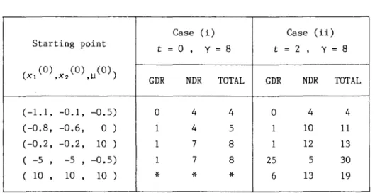
For Problem 1, we set the penalty parameter y

=

8 and tested the method using several starting points for t

=

0 and t

=

2 . For Problems 2, 3 and

4, we selected the same starting point x. (0) 2 i 1, •.. ,n

~

~j (0) 0 j 1, ... ,m

as in [4], and carried out the experiments for several values of t and y •

The computational results are shown in Tables 1 - 4. In the Tables, GDR, NDR and TOTAL represent the number of steepest ascent iterations, the number of Lagrange Newton iterations and the total number of iterations, respectively, and the symbol

*

indicates that convergence to the solution was not obtained within 30 iterations.

Note that, in Table 1, the starting point (-0.8, -0.6) is on the con-straint boundary of Problem 1. In such a case, the unit step size usually increases the value of nonsmooth exact penalty functions when the penalty con-stant is chosen very large, and convergence occurs at a very slow rate [9]. However, Table 1 shows that the differentiable exact penalty functions do not suffer from such a difficulty. On the other hand, it has been observed that, when a starting point is chosen near the global maximum

x*

=

(1, 0) or an initial estimate of Lagrange multiplier is set at a negative value, the generated sequence sometimes tends toward the global maximum or jams at a nonoptimal point.

As shown in Table 2, when t

=

0 , the method fails to converge to the solution of Problem 2. This is because "12

_xx

L(x*

_'

~*) is not positive defi-nite, and hence there is a duality gap between the original problem and its Wolfe dual (see Section 2). Thus, dual differentiable exact penalty functions of Han - Mangasarian type [12], which correspond to the case

t o ,

are only suitable to problems with positive definite 'V~xL(x*,~*) By virtue of Theorem 4, this difficulty could be overcome by selecting the value of t large enough. In fact, the results shown in Table 2 indicate that the value of t

=

2 is sufficient to obtain convergence.

Tables 3 and 4 reveal that all tested values of t (including t == 0 ) resulted in convergence to the solution for Problems 3 and 4. Moreover, i t is seen that the number of iterations required tends to increase as the value of t becomes large. The reason for this seems to be that, for those problems where Lagrangian itself is locally convex with respect to x at (x*,~*)

,

adding the term

t

Ilh(x) 112

usually makes conditions of the problems worse. Nevertheless, rapid convergence has been obtained for each problem in compari-son with the results reported by Di Pillo and Grippo [4] who applied the conjugate gradient method to minimize their exact penalty function directly.

314 M Fukushima, E. Yamakawa and H. Mine

Table 1. Results for Problem 1

Case (i) Case (ii)

Starting point t

=

0 , y

=

8 t

=

2

,

Y

=

8 ( (0) (0) (0)) Xl ,X2 ,11 _{GDR NDR TOTAL} GDR NDR TOTAL (-1.1, -0.1, -0.5) 0 4 4 0 4 4 (-0.8, -0.6,

o )

1 4 5 1 10 11 (-0.2, -0.2, 10 ) 1 7 8 1 12 13 ( -5

,

-5 , -0.5) 1 7 8 25 5 30 ( 10

,

10

,

10)

_*

_*

_*

6 13 19

Table 2. Results for Problem 2

t _Y GDR NDR TOTAL

0 16

_*

_*

_*

2 16 4 5 9

2 4 3 6 9

4 4 7 5 12

Table 3. Results for Problem 3 Table 4. Results for Problem 4

t Y GDR NDR TOTAL t Y GDR NDR TOTAL

0 16 0 8 8 0 4 0 3 3

0.25 16 2 7 9 2 4 1 4 5

0.25 32 3 7 10 2 16 2 5 7

7. Conclusion

We have considered the dual differentiable exact penalty functions in the context of general augmented Lagrangians on which several existing exact penalty functions are based. In particular, we have pointed out that various types of smooth exact penalty functions own some significant properties in common and differ only in the manner of choosing penalty parameters of the augmented Lagrangian.

References

[1] Bertsekas, D.P. Enlarging the Region of Convergence of Newton's Method for Constrained Optimization. Journal of Optimization Theory and Appli-cations, Vol. 36 (1982), 221-252.

[2] Bertsekas, D.P. Constrained Optimization and Lagrange Multiplier Methods. Academic Press, New York, 1982.

[3] Boggs, P.T. and Tolle, J.W. Augmented Lagrangians Which are Quadratic in the Multiplier. Journal of Optimization Theory and Applications,

Vol. 31 (1980), 17-26.

[4] Di Pillo, G. and Grippo, L. A New Class of Augmented Lagrangians in Nonlinear Programming. SIAM Journal on Control and Optimization, Vol. 17 (1979), 618-628.

[5] Di Pillo, G. and Grippo, L. : A Continuously Differentiable Exact Penalty Function for Nonlinear Programming Problems with Inequality Constraints.

SIAM Journal on Control and Optimization, Vol. 23 (1985), 72-84.

[6] Fiacco, A.V. and McCormick, G.P. Nonlinear Programming: Sequential Unconstrained Minimization Techniques. John Wiley

&

Sons, New York,

1968.

[7] Fletcher, R. A Class of Methods for Nonlinear Programming with Termi-nation and Convergence Properties. Integer and Nonlinear Programming,

(ed. J. Abadie). North-Holland, Amsterdam, 1970, 157-175.

[8] Fletcher, R. Practical Methods of Optimization, Volume 2: Constniined Optimization. John Wiley & Sons, Chichester, 1981.

[9] Fletcher, R. Penalty Functions. Mathematical Programming f The State

of the Art, Bonn, 1982, (eds. A. Bachem, M. Grotschel and B. Korte). Springer-Verlag, Berlin, 1983, 87-114.

[10] Fujiwara, 0., Han, S.-P. and Mangasarian, O.L. : Local Duality of Non-linear Programs. SIAM Journal on Control and Optimization, Vol. 22 (1984), 162-169.

316 M. Fukushima, E. Yamakawa and H. Mine

[11] Han, S.-P. and Mangasarian, O.L. : Exact Penalty Functions in Nonlinear Programming. Mathematical Programming, Vol. 17 (1979), 251-269.

[12] Han, S.-P. and Mangasarian, O.L. : A Dual Differentiable Exact Penalty Function. Mathematical Programming, Vol. 25 (1983), 293-306.

[13] Luenberger, D.G. : Introduction to Linear and Nonlinear Programming.

Addison-Wesley, Reading, Massachusetts, 1973.

[14] Mangasarian, O.L. Nonlinear Programming. McGraw-Hill, New York, 1969. [15] Ortega, J.M. and Rheinboldt,

w.e.

Iterative Solution of Nonlinear

Equations in Several Variables. Academic Press, New York, 1970.

[16] Zangwill, W.I. : Nonlinear Programming via Penalty Functions. Management Science, Vol. 13 (1967), 344-358.

[17] Zhadan, V.G. Modified Lagrange Functions in Nonlinear Programming.

USSR Computational Mathematics and Mathematical Physics (English Transla-tion), Vol. 22, No. 2 (1982), 43-57.

Masao FUKUSHIMA: Department of Applied Mathematics and Physics, Faculty of Engineering, Kyoto University, Kyoto, 606 Japan