Vol. 58, No. 3, July 2015, pp. 271–290
STABILITY IN SUPPLY CHAIN NETWORKS: AN APPROACH BY DISCRETE CONVEX ANALYSIS
Yoshiko T Ikebe Akihisa Tamura
Tokyo University of Science Keio University
(Received September 5, 2014; Revised February 28, 2015)
Abstract Ostrovsky generalized the stable marriage model of Gale and Shapley to a model on an acyclic directed graph, and showed the existence of a chain stable allocation under the conditions called same-side substitutability and cross-same-side complementarity. In this paper, we extend Ostrovsky’s model and the concepts of same-side substitutability and cross-side complementarity by using value functions which are defined on integral vectors and allow indifference. We give a characterization of chain stability under the extended versions of same-side substitutability and cross-side complementarity, and develop an algorithm which always finds a chain stable allocation. We also verify that twisted M♮-concave functions, which are variants of M♮-concave functions central to discrete convex analysis, satisfy these extended conditions. For twisted M♮-concave value functions of the agents, we analyze the time-complexity of our algorithm.
Keywords: Economics, stability, acyclic networks, discrete convex analysis
1. Introduction
Since the seminal paper by Gale and Shapley [9] the stable marriage model has been widely studied in such fields as economics, operations research, computer science and mathematics. Applications to various real world problems have been highly successful, e.g. the matching market for American physicians in Roth and Peranson [22], school choice in Abdulkadiro˘glu and S¨onmez [1], while theoretic aspects, particularly in game theory have also been studied (Roth and Sotomayor [23]). Extensions of this problem have been introduced in various settings. In economic theory, Kelso and Crawford [14] showed the existence of a stable allocation in the many-to-one job matching model, if value functions of firms have the gross substitutes condition. In computer science, Gusfield and Irving [10] developed efficient algorithms for several optimization problems on the stable marriage model. On the other hand, the maximum stable marriage problem with incomplete lists and ties was shown to be NP-hard by Iwama et al. [12]. For the above problem and some variations, approximation algorithms have been developed (see e.g., Iwama et al. [13] and McDermid [15].) Proofs of existence of a stable marriage/allocation for various generalizations have been made using Tarski’s fixed point theorem [28] by Adachi [2], Fleiner [5], Hatfield and Milgrom [11]. In operations research, the recent development of frameworks in discrete optimization have led to further models of increasing generality. Fleiner [4] extended the stable marriage model to the framework of matroids, showed existence of a stable allocation, Eguchi, Fujishige and Tamura [3] extended the matroidal model to the framework of discrete convex analysis, a field developed by Murota [17, 18] as a unified framework of discrete optimization. Fujishige and Tamura [7, 8] also gave a common generalization of the stable marriage model and the assignment model of Shapley and Shubik [24], by applying discrete convex analysis.
market model (mathematically modeled on a bipartite graph) to a supply chain network model (mathematically modeled on an acyclic directed graph.) The model is based on a supply chain with various agents (e.g. manufacturers, brokers, consumers), who conduct bilateral transactions of various commodities. The model is described by an acyclic directed graph with parallel edges, where vertices correspond to agents, and edges to the possible transactions of one unit of a certain commodity. Preferences of agents are described by choice functions on subsets of edges. In this setting, stable matchings are generalized to ‘chain stable allocations.’ Ostrovsky [21] newly defined the concepts of same-side substitutability and cross-side complementarity, and proved that if choice functions of the agents satisfy these two conditions then there always exists a chain stable allocation, (see the next section for details.) Fleiner [6] also imported the concept of stability into the discrete/continuous flow problem, and generalized the lattice structure of stable marriages.
In this paper, we extend Ostrovsky’s model and the concepts of same-side substitutability (SSS) and cross-side complementarity (CSC) by using value functions which are defined on integral vectors and allow indifference. We give a characterization of chain stability under the extended SSS and CSC. Our main result is that there always exists a chain stable allocation when value functions satisfy the extended SSS and CSC. We show this by giving an algorithm for finding a chain stable allocation together with certificates of stability. We also illustrate that value functions satisfying SSS and CSC are natural in the discrete convex analysis framework, by showing that twisted M♮-concave functions, a variant of M♮-concave
functions, satisfy both extended SSS and CSC. We also give analysis of the time-complexities of our algorithms when the value functions of agents satisfy twisted M♮-concavity. The merit of utilizing discrete convex analysis, is that one can easily image and construct concrete examples of choice functions and value functions satisfying SSS and CSC.
This paper is organized as follows. In Section 2, we describe Ostrovsky’s supply chain model and extend SSS and CSC, and in Section 3 we define twisted M♮-concave function,
give some examples, and prove that twisted M♮-concave functions satisfy the extended SSS and CSC. We modify Ostrovsky’s model and chain stability in terms of value functions, and show a characterization of chain stable allocations in Section 4. Finally, in Sections 5 and 6, we develop an algorithm for finding a chain stable allocation, and analyze its time complexity when agents’ value functions are twisted M♮-concave.
2. Same-Side Substitutability and Cross-Side Complementarity
In this section, we briefly describe Ostrovsky’s supply chain network model [21], and extend the concepts of same-side substitutability and cross-side complementarity.
The model in Ostrovsky [21] is based on a supply chain with various agents (e.g. manu-facturers, brokers, consumers), who conduct bilateral transactions of various commodities. Each commodity is traded discretely in units, and the buyer pays the seller some price, which depends on the number of units changing hands. For instance, transaction of only one unit of a certain commodity may cost the buyer 10, while purchase of two units will cost 18, and three units 24. This situation is represented by an acyclic directed graph with parallel edges. Each vertex corresponds to an agent, and each edge to the possible transac-tion of one unit of a certain commodity. More precisely, a directed edge is associated with a
contract consisting of the seller (understood to be the tail), the buyer (corresponding to the
head), an identifier specifying the commodity together with the ‘serial number’ of the unit being traded, and the price accompanying the transaction. Thus, if some agent u is willing to sell to another agent v, up to three units of commodity A at the prices mentioned above,
and up to two units of commodity B at 15 each, there will be five contracts represented by edges from u to v, the first for the sale of the first unit of A with price 10, the second for the second unit of A with price 18− 10 = 8, and so on with the fifth standing for the second unit of B with price 15. An allocation of this model is specified by a set of contracts. As is in case of brokers who buy from manufacturers, and sell to consumers, each agent can participate in multiple contracts, some as the buyer, and others as the seller, as long as no agent is involved in two contracts of the same unit (with the same serial number) of commodity which differ only in price.
For an allocation X, let Xu be the set of contracts involving agent u as either seller or
buyer. For any given X, each u has a choice function which specifies his/her most desirable subset of X, this is denoted by Chu(X)⊆ Xu. In these choice functions, contracts involving
differing units of the same commodity are assumed to be preferred in lexicographical order, and indifference is not allowed, so that for any X, Chu(X) is uniquely determined.
The key concepts in Ostrovsky [21], are same-side substitutability and cross-side com-plementarity. For an agent u, denote by Xu− the contracts of X in which u is a buyer, and
X+
u the contracts of X for which u is a seller. The preferences of agent u are same-side
substitutable if
• for any allocations X and Y , with X+
u = Yu+ and Xu− ⊆ Yu−,
Xu−\ (Chu(X))−u ⊆ Yu−\ (Chu(Y ))−u, (2.1)
• for any allocations X and Y , with X+
u ⊆ Yu+ and Xu− = Yu−,
Xu+\ (Chu(X))+u ⊆ Y
+
u \ (Chu(Y ))+u. (2.2)
It is easy to show that (2.1) and (2.2) are equivalent to Xu− ∩ (Chu(Y ))−u ⊆ (Chu(X))−u
and X+
u ∩ (Chu(Y ))+u ⊆ (Chu(X))+u, respectively. The preferences of agent u are cross-side
complementary if
• for any allocations X and Y , with X+
u = Yu+ and Xu− ⊆ Yu−,
(Chu(X))+u ⊆ (Chu(Y ))+u, (2.3)
• for any allocations X and Y , with X+
u ⊆ Yu+ and Xu− = Yu−,
(Chu(X))−u ⊆ (Chu(Y ))−u. (2.4)
Presented with a larger set of contracts on one side, same-side substitutability says that the agent will not accept any contract on that side that was rejected in the smaller set, and cross-side complementarity that no contract on the opposite side that was previously accepted will be rejected.
We now extend same-side substitutability (SSS) and cross-side complementarity (CSC) of Ostrovsky [21] to the case where value functions representing preferences of agents are defined on integral vectors and allow indifference.
Let E be a nonempty finite set, andZ and R be the sets of integers and reals, respectively. We denote by ZE the set of integral vectors x = (x(e) : e ∈ E) indexed by E, where x(e) denotes the e-th component of vector x. Here E and x ∈ ZE might denote the set of
indivisible commodities and the numbers x(e) of commodities e sold or bought by an agent. The value function of each agent is defined as a function f : ZE → R ∪ {−∞}. The
effective domain of f is defined by
and the set of maximizers of f on U ⊆ ZE by
argmax{f(y) | y ∈ U} = {x ∈ U | f(x) ≥ f(y) (∀y ∈ U)}. We assume that each value function f satisfies the following assumption:
(A) dom f is bounded and has 0 as the minimum point.
The boundedness of effective domains implies that a budget constraint is implicitly imposed on each agent’s value function. We note that under the assumption, argmax{f(y) | y ∈ U} is well-defined if U ∩ dom f ̸= ∅. We can define a choice correspondence Cf by using the
value function f as:
Cf(q) = argmax{f(y) | y ≤ q} (q ∈ ZE),
where q denotes possible quotas of commodities.
For any x, y ∈ ZE, the vectors x∧ y and x ∨ y in ZE are defined by
(x∧ y)(e) = min{x(e), y(e)}, (x ∨ y)(e) = max{x(e), y(e)} (e ∈ E).
In order to define (SSS) and (CSC) for value functions, we assume that E is partitioned into
E+ and E−, i.e., E = E+∪ E− and E+∩ E− =∅. For any vector x ∈ ZE, we respectively
denote by x+and x− the subvectors of x on E+ and E−. The following property is a natural extension of (SSS) and (CSC). We say that a value function f : ZE → R ∪ {−∞} satisfies
SSS-CSC property on (E+, E−) if the following conditions hold for any vectors z
1, z2 ∈ ZE with z1 ≥ z2 ≥ 0,
(a) if z1+ ≥ z2+ and z−1 = z2− then
• for any x1 ∈ argmax{f(y) | y ≤ z1}, there exists x2 ∈ argmax{f(y) | y ≤ z2} such that
z2+∧ x+1 ≤ x+2 and x−2 ≤ x−1, (2.5)
• for any x2 ∈ argmax{f(y) | y ≤ z2}, there exists x1 ∈ argmax{f(y) | y ≤ z1} with (2.5),
(b) if z1+ = z+2 and z1− ≥ z2− then
• for any x1 ∈ argmax{f(y) | y ≤ z1}, there exists x2 ∈ argmax{f(y) | y ≤ z2} such that
z2−∧ x−1 ≤ x−2 and x+2 ≤ x+1, (2.6)
• for any x2 ∈ argmax{f(y) | y ≤ z2}, there exists x1 ∈ argmax{f(y) | y ≤ z1} with (2.6).
We will give a class of functions with SSS-CSC property in the next section.
A value function with SSS-CSC property has the following properties, which are used in Sections 4 and 5.
Lemma 2.1. Let f : ZE → R ∪ {−∞} be a function with SSS-CSC property on (E+, E−) and x, z1, z2 ∈ ZE be such that x ∈ argmax{f(y) | y ≤ z1}, and x ∈ argmax{f(y) | y ≤ z2}. If argmax{f(y) | y ≤ z1 ∨ z2} ̸= ∅ and either z+1 = z
+
2 or z−1 = z2− then we have x∈ argmax{f(y) | y ≤ z1∨ z2}.
Proof. We will prove the case where z1+ = z2+ (we can prove the case z1− = z2− similarly.) Let z3 = z1 ∨ z2. Since z3+ = z
+
2 and z3− ≥ z2−, by (b) in SSS-CSC property, there exists x3 ∈ argmax{f(y) | y ≤ z3} such that z2−∧ x−3 ≤ x− and x+ ≤ x+3. For each e ∈ E−, the first inequality means x3−(e) ≤ x−(e) if x−(e) < z2−(e); otherwise x−3(e) ≤ z1−(e) because
x−(e) = z−2(e), x≤ z1∧ z2 and x3 ≤ z1∨ z2. Thus, we have x−3 ≤ z−1. Since x + 3 ≤ z + 3 = z + 1 obviously holds, we have x3 ∈ argmax{f(y) | y ≤ z1}, which implies f(x) = f(x3) and also x∈ argmax{f(y) | y ≤ z3}.
Lemma 2.2. Let f : ZE → R ∪ {−∞} be a function with SSS-CSC property on (E+, E−) and x, z1, z2 ∈ ZE be such that z1 ≥ z2, argmax{f(y) | y ≤ z1} ̸= ∅, and x ∈ argmax{f(y) | y ≤ z2}. If for each e ∈ E, x(e) < z2(e) whenever z2(e) < z1(e) then we have x ∈ argmax{f(y) | y ≤ z1}.
Proof. Let z3 be the vector defined by z+3 = z +
2 and z3− = z1−. By (b) in SSS-CSC property for z3, z2 and x, there exists x3 ∈ argmax{f(y) | y ≤ z3} such that z−2 ∧ x−3 ≤ x− and x+ ≤ x+3. For each e ∈ E− with z2−(e) < z1−(e), we have x(e) < z2(e) from the assumption, and hence, x−3(e) ≤ x−(e) from the first inequality z−2 ∧ x−3 ≤ x−. For each e ∈ E− with
z2−(e) = z1−(e), the first inequality together with x−3(e) ≤ z−3(e) = z−1(e) = z2−(e) means
x−3(e)≤ x−(e). Thus, we have x−3 ≤ z2−. Since x+3 ≤ z3+ = z2+ obviously holds, we have x3 ∈ argmax{f(y) | y ≤ z2}, which implies f(x) = f(x3) and also x∈ argmax{f(y) | y ≤ z3}.
Since z1+ ≥ z3+ and z1− = z3− hold, by using (a) in SSS-CSC property for z1, z3, and x, we can show x∈ argmax{f(y) | y ≤ z1} in precisely the same way as above.
3. M♮-Concave Functions and Twisted M♮-Concave Functions
In this section, we give a useful class of functions with SSS-CSC property.
Let E be a nonempty finite set. Given a vector x∈ ZE, its positive support and negative
support are defined by
supp+(x) ={e ∈ E | x(e) > 0}, supp−(x) ={e ∈ E | x(e) < 0}.
For each S ⊆ E, we denote by χS the characteristic vector of S defined by χS(e) = 1 if
e∈ S; otherwise 0, and simply write χe instead of χ{e} for each e∈ E.
An M-concave function defined by Murota [17, 18] is a function f : ZE → R ∪ {−∞}
with dom f ̸= ∅ satisfying
(M-EXC) ∀x, y ∈ dom f, ∀e ∈ supp+(x− y), ∃e′ ∈ supp−(x− y) : f (x) + f (y)≤ f(x − χe+ χe′) + f (y + χe− χe′).
From (M-EXC), the effective domain of an M-concave function lies on a hyperplane {y ∈ RE | y(E) = constant}, where y(E) =P
e∈Ey(e).
The concept of M♮-concavity which is a variant of M-concavity was proposed by Murota
and Shioura [20]. Let 0 denote a new element not in E and define eE ={0} ∪ E. A function f : ZE → R ∪ {−∞} with dom f ̸= ∅ is called M♮-concave if it is expressed in terms of an
M-concave function ef :ZEe → R ∪ {−∞} as: for all x ∈ ZE
f (x) = ef (x0, x) with x0 =−x(E).
Namely, an M♮-concave function is a function obtained as the projection of an M-concave
function. Conversely, an M♮-concave function f determines the corresponding M-concave function ef by e f (x0, x) = ½ f (x) (x0 =−x(E)) −∞ (otherwise) ((x0, x)∈ Z e E ).
Theorem 3.1 (Murota and Shioura [20]). A function f :ZE → R ∪ {−∞} with dom f ̸= ∅
is M♮-concave if and only if it satisfies
(M♮-EXC) ∀x, y ∈ dom f, ∀e ∈ supp+(x− y), ∃e′ ∈ supp−(x− y) ∪ {0} :
f (x) + f (y)≤ f(x − χe+ χe′) + f (y + χe− χe′),
where we assume χ0 is the zero vector on E.
An M♮-concave function has nice features as a value function, e.g., submodularity, natural
generalizations of gross substitutability, single improvement property and substitutability (see Murota [19], Fujishige and Tamura [8] for details.)
As in Section 2, let E+and E−be a partition of E (i.e. E = E+∪E−and E+∩E− =∅) and for x = (x+, x−)∈ ZE, define tw(x)∈ ZE by (x+,−x−). Let f :ZE → R ∪ {−∞} be a function defined by
f (x) = bf (tw(x)) (x∈ ZE) (3.1)
for some M♮-concave function bf . We call a function defined as above a twisted M♮-concave
function on (E+, E−). Note that if either E+ = ∅ or E− = ∅ then twisted M♮-concave
functions are also M♮-concave. Twisted M♮-concave functions are generalizations of the class of functions called GM-concave functions in Sun and Yang [26]. We give some simple examples of M♮-concave and twisted M♮-concave functions.
Example 3.1. We call a nonempty familyT of subsets of E a laminar family if X ∩Y = ∅, X ⊆ Y or Y ⊆ X holds for every X, Y ∈ T . For a laminar family T and a family of univariate concave functions fY : R → R ∪ {−∞} indexed by Y ∈ T , the function
f :ZE → R ∪ {−∞} defined by
f (x) = X
Y∈T
fY (x(Y )) (x∈ ZE)
is called a laminar concave function. It is known that a laminar concave function is M♮ -concave if dom f ̸= ∅ (see Murota [19].) For a partition (E+, E−) of E, the function defined by g(x) = ½ 0 (x≥ 0, x(E−) = x(E+)) −∞ (otherwise) (x∈ Z E)
is twisted M♮-concave on (E+, E−) because g corresponds to the laminar concave function with the laminar family E∪ {E} and the following univariate concave functions: for each e∈ E+, bge(y) = ½ 0 (y ≥ 0) −∞ (otherwise) (y ∈ R), for each e∈ E−, bge(y) = ½ 0 (y ≤ 0) −∞ (otherwise) (y ∈ R), and for E, bgE(y) = ½ 0 (y = 0) −∞ (otherwise) (y ∈ R).
Similarly, the function defined by h(x) =
½
x(E−)− x(E+) (x≥ 0, x(E−)≥ x(E+))
−∞ (otherwise) (x∈ Z
is also twisted M♮-concave on (E+, E−). If E− and E+ respectively denote the input com-modities and output comcom-modities, function g can be used to enforce the conservation between input and output commodities, and h can be used to forbid the total of output commodities to exceed that of the input commodities. //
Example 3.2. Let f be a twisted M♮-concave function on (E+, E−), and bf its corresponding M♮-concave function. For any two vectors a, b∈ ZE with a≤ b, the function defined by
b f[a,b](x) = ½ bf (x) (a≤ x ≤ b) −∞ (otherwise) (x∈ Z E )
is also M♮-concave if dom bf
[a,b]̸= ∅ (see Murota [19].) Hence the function defined by
f[a,b](x) = ½
f (x) (a≤ x ≤ b)
−∞ (otherwise) (x∈ Z
E)
is also twisted M♮-concave if dom f[a,b] ̸= ∅. //
Example 3.3. Let f be a twisted M♮-concave function on (E+, E−), and bf its corresponding M♮-concave function. Given univariate concave functions f
e : R → R ∪ {−∞} indexed by e∈ E, it is known that b f (x) +X e∈E fe(x(e)) (x∈ ZE)
is also M♮-concave if its effective domain is nonempty (see Murota [19].) This says that the
sum of an M♮-concave function and a separable concave function is also M♮-concave. Hence
the sum of a twisted M♮-concave function and a separable concave function, i.e., f (x) +X
e∈E
fe(x(e)) (x∈ ZE)
is also twisted M♮-concave if its effective domain is nonempty. //
The next two lemmas, namely, Lemma 3.1 and Lemma 3.2, say that twisted M♮-concave functions satisfy SSS-CSC property on (E+, E−).
Lemma 3.1. Let f : ZE → R ∪ {−∞} be a twisted M♮-concave function on (E+, E−) and z1, z2 ∈ ZE be such that z1+ ≥ z
+
2, z1− = z−2, argmax{f(y) | y ≤ z1} ̸= ∅, and argmax{f(y) | y≤ z2} ̸= ∅.
(a) For any x1 ∈ argmax{f(y) | y ≤ z1}, there exists x2 ∈ argmax{f(y) | y ≤ z2} such that z2+∧ x+1 ≤ x+2 and x−2 ≤ x−1. (3.2) (b) For any x2 ∈ argmax{f(y) | y ≤ z2}, there exists x1 ∈ argmax{f(y) | y ≤ z1} with
(3.2).
Proof. Let bf be an M♮-concave function satisfying (3.1).
We begin by making some observations on a pair x1, x2 with x1 ∈ argmax{f(y) | y ≤ z1} and x2 ∈ argmax{f(y) | y ≤ z2} not satisfying (3.2). Since (3.2) does not hold, there must exist e ∈ E such that either min{z2+(e), x+1(e)} > x+2(e) or x−2(e) > x−1(e). In the former case we have e∈ E+, z2(e) > x2(e) and x1(e) > x2(e), and in the latter case we have e∈ E−
and x2(e) > x1(e). In both cases, e∈ supp+(tw(x1)− tw(x2)) must hold. By (M♮-EXC) for b
f , there exists e′ ∈ supp−(tw(x1)− tw(x2))∪ {0} such that b
f (tw(x1)) + bf (tw(x2))≤ bf (tw(x1)− χe+ χe′) + bf (tw(x2) + χe− χe′). (3.3)
Let ex1 = tw(tw(x1)− χe+ χe′) and ex2 = tw(tw(x2) + χe − χe′). If e ∈ E+ then ex1(e) = x1(e)− 1 ≤ z1(e) and ex2(e) = x2(e) + 1 ≤ z2(e) hold; otherwise, ex1(e) = x1(e) + 1 ≤ x2(e) ≤ z2(e) = z1(e) and ex2(e) = x2(e)− 1 ≤ z2(e). If e′ ∈ E+ then we have ex1(e′) = x1(e′) + 1≤ x2(e′)≤ z2(e′)≤ z1(e′) andex2(e′) = x2(e′)−1 ≤ z2(e′). If e′ ∈ E− then we have ex1(e′) = x1(e′)− 1 ≤ z1(e′) and ex2(e′) = x2(e′) + 1≤ x1(e′)≤ z1(e′) = z2(e′). Hence ex1 ≤ z1 and ex2 ≤ z2 hold whichever e′ belongs to. Recalling that x1 ∈ argmax{f(y) | y ≤ z1} we have f (x1)≥ f(ex1), which implies bf (tw(x1))≥ bf (tw(x1)− χe+ χe′), which considered
together with (3.3), in turn yields bf (tw(x2))≤ bf (tw(x2) + χe− χe′), i.e., f (x2)≤ f(ex2) and hence ex2 ∈ argmax{f(y) | y ≤ z2}. Applying the same argument to x2 and ex1, we obtain that ex1 ∈ argmax{f(y) | y ≤ z1}.
To prove (a), we consider x1 ∈ argmax{f(y) | y ≤ z1} to be fixed, and choose x2 to be an element in argmax{f(y) | y ≤ z2} that minimizes
X
{x1(e)−x2(e)| e ∈ supp+((z2+∧x + 1)−x
+ 2)} +
X
{x2(e)−x1(e)| e ∈ supp+(x−2−x−1)}. (3.4) For such x2, (3.2) must hold, since otherwise, for ex2 defined as above, ex2 ∈ argmax{f(y) | y≤ z2}, and the value of (3.4) for x1 and ex2 is smaller by exactly one than that for x1 and x2, which is a contradiction.
Similarly, for fixed x2 ∈ argmax{f(y) | y ≤ z2}, any x1 in argmax{f(y) | y ≤ z1} minimizing (3.4), satisfies (3.2), proving (b).
We can show the following lemma in the same way as Lemma 3.1.
Lemma 3.2. Let f : ZE → R ∪ {−∞} be a twisted M♮-concave function on (E+, E−) and
z1, z2 ∈ ZE be such that z1+ = z +
2, z1−≥ z−2, argmax{f(y) | y ≤ z1} ̸= ∅, and argmax{f(y) | y≤ z2} ̸= ∅.
(a) For any x1 ∈ argmax{f(y) | y ≤ z1}, there exists x2 ∈ argmax{f(y) | y ≤ z2} such that z2−∧ x−1 ≤ x−2 and x+2 ≤ x+1. (3.5) (b) For any x2 ∈ argmax{f(y) | y ≤ z2}, there exists x1 ∈ argmax{f(y) | y ≤ z1} with
(3.5).
4. Our Model
Let G = (V, E) be an acyclic directed graph. For each v ∈ V , let δ(v), δ+(v) and δ−(v) respectively denote the set of all edges incident to v, the set of outgoing edges from v and the set of incoming edges to v. As in Ostrovsky [21], the vertex set corresponds to the agents (e.g. manufacturers, brokers, consumers) involved in a supply chain, and the edge set represents possible transactions of commodities. However, instead of creating multiple edges to deal with different units of the same commodity, we use integral vectors defined on the edge set. Each agent v∈ V has a value function fv on δ(v), i.e., fv :Zδ(v) → R ∪ {−∞}.
We recall that each value function fv satisfies Assumption (A). We call x∈ ZE an allocation.
For each allocation x and agent v ∈ V , xδ(v) denotes the subvector (x(e) : e ∈ δ(v)) of x.
feasible allocation x is individually rational if fv(xδ(v)) = max{fv(y) | y ≤ xδ(v)} for all
v ∈ V . Individual rationality means that no agent would like to unilaterally decrease the
number of units in any transaction he/she participates in. For a feasible allocation x∈ ZE,
a blocking path for x is a directed path P = (v0, e1, v1, e2, . . . , ek, vk) such that
• fv0(xδ(v0)) < max{fv0(y)| y ≤ (x + χe1)δ(v0)},
• fvi(xδ(vi)) < max{fvi(y)| y ≤ (x+χei+χei+1)δ(vi), y(ei) = x(ei)+1, y(ei+1) = x(ei+1)+1}
for i = 1, . . . , k− 1,
• fvk(xδ(vk)) < max{fvk(y)| y ≤ (x + χek)δ(vk)}.
We say that a feasible allocation x∗ is chain stable or simply stable if it is individually rational and has no blocking path. Blocking paths are generalizations of blocking pairs in stable matchings, and represent a sequence of agents, each one buying from the previous and selling to the next, who would like to increase their transactions by one unit each (and possibly decrease other deals.)
We give a sufficient condition for a given allocation x∗ ∈ ZE to be chain stable.
Lemma 4.1. For a feasible allocation x∗ ∈ ZE, if there exist z, z ∈ (Z ∪ {+∞})E such that
x∗δ(v) ∈ argmax{fv(y)| yδ+(v) ≤ zδ+(v), yδ−(v) ≤ zδ−(v)} (v ∈ V ), (4.1)
z(e) = +∞ or z(e) = +∞ (e ∈ E), (4.2)
then x∗ is chain stable.
Proof. Condition (4.1) guarantees that x∗ is individually rational. Suppose, to the contrary, that there is a blocking path P = (v0, e1, v1, e2, . . . , ek, vk). By the condition for v0 in the definition of a blocking path together with (4.1), z(e1) = x∗(e1) must hold, which implies z(e1) = +∞ by (4.2). For agent v1, we have e1 ∈ δ−(v1), e2 ∈ δ+(v1), x∗δ+(v
1) ≤ zδ+(v1),
(x∗+ χe1)δ−(v1) ≤ zδ−(v1) and
fv1(x∗δ(v1)) < max{fv1(y)| y ≤ (x∗+χe1+χe2)δ(v1), y(e1) = x∗(e1)+1, y(e2) = x∗(e2)+1},
fv1(x ∗
δ(v1)) = max{fv1(y)| yδ+(v1)≤ zδ+(v1), yδ−(v1)≤ zδ−(v1)}.
Thus z(e2) = x∗(e2) must hold, and hence, z(e2) = +∞ by (4.2). In the same way as above, we obtain z(ei) = x∗(ei) and z(ei) = +∞ for i = 1, 2, . . . , k. Since ek ∈ δ−(vk) and
z(ek) = +∞, the condition for vk in the definition of a blocking path, i.e., fvk(x∗δ(vk)) <
max{fvk(y) | y ≤ (x
∗+ χ
ek)δ(vk)} contradicts (4.1) for vk. Hence there is no blocking path
for x∗, and hence, x∗ must be chain stable.
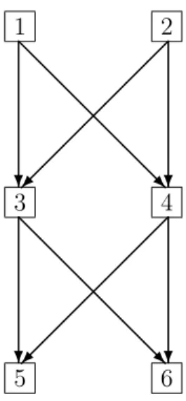
Example 4.1. We consider the supply chain network in Figure 1 in which agents 1 and 2 are producers, agents 3 and 4 brokers, and agents 5 and 6 consumers. Note that transactions can only occur between producers and brokers, and brokers and consumers. We assume that
• producers 1 and 2 respectively supply 5 and 7 homogeneous commodities per week, • each producer wants to sell (to brokers) primarily as many commodities as possible, and
secondly the same amounts as possible,
• each broker must sell all commodities he/she bought, within this condition each wants to primarily buy and sell as many commodities as possible, and secondly to buy from producers and sell to consumers the same amounts as possible,
• each consumer can buy up to 5 commodities; within this limit each wants to buy primarily as many commodities as possible, and secondly the same amounts as possible.
1 2 3 4 5 6 ? @ @ @ @ @ @ @ R ? ? @ @ @ @ @ @ @ R ?
Figure 1: An example of supply chain network: 1 and 2 are producers, 3 and 4 brokers, and 5 and 6 consumers.
Let xab be a variable representing the number of commodities traded between agents a and
b. In order to describe preferences of the producers and consumers, we adopt the following M♮-concave function gα :Z2 → R ∪ {−∞} defined for integer α:
gα(y1, y2) = ½
0 (y1, y2 ≥ 0, y1+ y2 ≤ α)
−∞ (otherwise) (y1, y2 ∈ Z).
By using gα and a sufficiently small positive value ε, we can describe preferences of agents
1, 2, 5 and 6 by using the following functions:
f1(x13, x14) = g5(x13, x14) + (x13+ x14)− ε(x213+ x 2 14) (x13, x14 ∈ Z), f2(x23, x24) = g7(x23, x24) + (x23+ x24)− ε(x223+ x 2 24) (x23, x24 ∈ Z), f5(x35, x45) = g5(x35, x45) + (x35+ x45)− ε(x235+ x245) (x35, x45 ∈ Z), f6(x36, x46) = g5(x36, x46) + (x36+ x46)− ε(x236+ x 2 46) (x36, x46 ∈ Z),
in which the second terms show preference to trade as many commodities as possible, and the third terms that they trade with the two brokers as the same amounts as possible. Functions f1, f2, f5 and f6 are M♮-concave (i.e., twisted M♮-concave) because these functions are the sums of M♮-concave function gα and separable concave functions (see Example 3.3.) In order
to describe preferences of the brokers, we use the following function h :Z4 → R ∪ {−∞}:
h(y1−, y2−, y+5, y+6) = ½ 0 (y1−, y−2, y5+, y6+≥ 0, y1−+y−2 = y5++y+6) −∞ (otherwise) (y − 1 , y2−, y + 5, y + 6 ∈ Z),
where h is the twisted M♮-concave shown in Example 3.1. By using h, we can describe preferences of agents 3 and 4 by using the following functions:
f3(x13, x23, x35, x36) = h(x13, x23, x35, x36) + (x13+x23−ε(x213+x 2 23)) + (x35+x36−ε(x235+x 2 36)) (x13, x23, x35, x36 ∈ Z), f4(x14, x24, x45, x46) = h(x14, x24, x45, x46) + (x14+x24−ε(x214+x224)) + (x45+x46−ε(x245+x246)) (x14, x24, x45, x46 ∈ Z).
In these functions, h enforces the conservation between input and output commodities, and the second and third terms describe the brokers’ preference. By Examples 3.1 and 3.3, f3 and f4 are twisted M♮-concave.
In the instance, let us consider the following allocations x and x∗.
(1, 3) (1, 4) (2, 3) (2, 4) (3, 5) (3, 6) (4, 5) (4, 6)
x 2 2 2 3 2 2 2 3
x∗ 2 3 2 3 2 2 3 3
z +∞ +∞ 2 3 2 2 3 3
z +∞ 3 +∞ +∞ +∞ +∞ +∞ +∞
Allocation x∗ is chain stable because x∗, z and z defined as above satisfy (4.1) and (4.2) in Lemma 4.1. On the other hand, x is not chain stable, because P = (1, (1, 3), 3, (3, 5), 5) is a blocking path for x. //
In general, conditions (4.1) and (4.2) might not be a necessary condition for which a feasible allocation is chain stable. In the sequel, we deal with the case where each value function fv satisfies SSS-CSC property on (δ+(v), δ−(v)). In this case, (4.1) and (4.2) are
a necessary condition for the chain stability of a feasible allocation x∗. To show this, we will first show that the following procedure decides whether a given individually rational allocation x∗ is chain stable or not.
Stability Check
input:
an individually rational allocation x∗∈ZE, i.e. x∗δ(v)∈argmax{fv(y)| y≤x∗δ(v)} for v∈V ;
output:
z, z ∈ (Z∪{+∞})E satisfying (4.1) and (4.2) if x∗ is stable; otherwise a blocking path;
Step 0.
O := E, I0 := I1 :=∅ and k := 1;
For v ∈ V and e = vw ∈ O ∩ δ+(v) with f
v(x∗δ(v)) < max{fv(y)| y ≤ (x∗+ χe)δ(v)},
· Ik := Ik∪ {e}, O := O \ {e};
· p(e) = nil,
· if fw(x∗δ(w)) < max{fw(y)| y ≤ (x∗+χe)δ(w)} then output blocking path P = (v, e, w)
for x∗ and stop,
k := 2, Ik := Ik−1;
Step 1.
For v ∈ V and e = vw ∈ O ∩ δ+(v) with f
v(x∗δ(v)) < max{fv(y)| y ≤ (x∗+χIk−1∩δ−(v)+ χe)δ(v)},
· Ik := Ik∪ {e}, O := O \ {e};
· select e′ ∈ (Ik−1\ Ik−2)∩ δ−(v) with
fv(x∗δ(v)) < max{fv(y)| y ≤ (x∗+χe′+χe)δ(v), y(e′) = x∗(e′)+1, y(e) = x∗(e)+1},
(we will show the existence of e′ later) and set p(e) := e′,
· if fw(x∗δ(w)) < max{fw(y)| y ≤ (x∗+ χe)δ(w)} then construct and output a path P
of length k by backtracking e, p(e), p(p(e)),· · · , and stop,
If Ik= Ik−1 then go to Step 2; otherwise k := k + 1, Ik:= Ik−1 and continue Step 1;
Step 2.
Output z and z defined by
z(e) := ½ x∗(e) (e∈ Ik) +∞ (e∈ O), z(e) := ½ +∞ (e∈ Ik) x∗(e) (e∈ O),
and stop.
Recall that each value function fv for v ∈ V satisfies SSS-CSC property on (δ+(v), δ−(v)).
Since set O is reduced by one element in Steps 0 and 1, Stability Check terminates in finite time. At the end of each iteration in Steps 0 and 1 of Stability Check, O and Ik
form a partition of E, i.e., E = O∪ Ik and O∩ Ik=∅, which imply that z and z in Step 2 are well-defined and satisfy (4.2).
If Stability Check stops in Step 0 then P = (v, e, w) is obviously a blocking path for
x∗. Hereafter, we consider the case where Step 1 is executed. Just after Step 0, for each
w∈ V , we have
x∗δ(w) ∈ max{fw(y)| y ≤ (x∗+ χe)δ(w)}
for all e∈ I1 ∩ δ−(w). By repeatedly using Lemma 2.1, we obtain that x∗δ(w) ∈ argmax{fw(y)| y ≤ (x∗+ χI1∩δ−(w))δ(w)} (w ∈ V ).
For k≥ 2, just before the iteration for k in Step 1, we assume that
x∗δ(v) ∈ argmax{fv(y)| y ≤ (x∗+ χIk−1∩δ−(v))δ(v)} (v ∈ V ) (4.3)
and consider the iteration for k in Step 1. We may abbreviate (χe)δ(v) as χe if e∈ δ(v), for
example, for y ∈ Zδ(v), we denote y + (χ
e)δ(v) by y + χe. Let v and e be a vertex and an
edge such that e = vw ∈ O ∩ δ+(v) and
fv(x∗δ(v)) < max{fv(y)| y ≤ (x∗+ χIk−1∩δ−(v)+ χe)δ(v)}. (4.4)
We claim that there is e′ ∈ (Ik−1\ Ik−2)∩ δ−(v) with
fv(x∗δ(v)) < max{fv(y)| y ≤ (x∗+ χe′+ χe)δ(v), y(e′) = x∗(e′) + 1, y(e) = x∗(e) + 1}. (4.5)
By the description of Stability Check,
x∗δ(v)∈ argmax{fv(y)| y ≤ (x∗+ χIk−2∩δ−(v)+ χe)δ(v)} (4.6)
must hold. From (4.6) and (b) in SSS-CSC property for
z1 = (x∗+ χIk−1∩δ−(v)+ χe)δ(v), z2 = (x∗+ χIk−2∩δ−(v)+ χe)δ(v), x2 = x∗δ(v),
there exists y∗ ∈ argmax{fv(y)| y ≤ (x∗+ χIk−1∩δ−(v) + χe)δ(v)} such that
(x∗+ χIk−2∩δ−(v)+ χe)δ−(v)∧ y∗δ−(v)≤ x∗δ−(v), which together with (4.4) implies
yI∗k−2∩δ−(v) ≤ x∗Ik−2∩δ−(v), y∗Ik−1∩δ−(v) ̸≤ x∗Ik−1∩δ−(v).
Let S = {e′′ ∈ (Ik−1\ Ik−2)∩ δ−(v)| y∗(e′′) = x∗(e′′) + 1}. Then, there exists e′ ∈ S such that
x∗δ(v)̸∈ argmax{fv(y)| y ≤ (x∗+ χIk−2∩δ−(v)+ χe′+ χe)δ(v)},
since otherwise, Lemma 2.1 implies x∗δ(v) ∈ argmax{fv(y)| y ≤ (x∗+χIk−2∩δ−(v)+χS+χe)δ(v)}
contradicting (4.4). In the same way as above, (b) in SSS-CSC property for (4.6) implies that there exists y′ such that
y′ ∈ argmax{fv(y)| y ≤ (x∗+ χIk−2∩δ−(v) + χe′ + χe)δ(v)},
It follows from (4.3) and (4.6) that y′(e) = x∗(e) + 1 and y′(e′) = x∗(e′) + 1, and hence, e′ has (4.5).
We assume that there exist v, w ∈ V and e = vw ∈ O ∩ δ+(v) such that f
v(x∗δ(v)) <
max{fv(y) | y ≤ (x∗ + χIk−1∩δ−(v) + χe)δ(v)} and fw(x∗δ(w)) < max{fw(y) | y ≤ (x∗ +
χe)δ(w)} in Step 1. By backtracking edges from e by using p, we can construct a path
P = (v0, e1, v1, . . . , ek−1 = p(e), vk−1 = v, ek = e, vk= w) such that
fv0(x ∗ δ(v0)) < max{fv0(y)| y ≤ (x + χe1)δ(v0)}, fvi(x ∗ δ(vi)) < max{fvi(y)| y ≤ (x ∗+χ ei+χei+1)δ(vi), y(ei) = x ∗(e
i)+1, y(ei+1) = x∗(ei+1)+1}
(i = 1, . . . , k−1), fvk(x ∗ δ(vk)) < max{fvk(y)| y ≤ (x ∗+ χ ek)δ(vk)}.
Hence P is a blocking path for x∗.
We next consider the situation just after the iteration for k (and before updating k) in Step 1. In the same way as the proof for the case just after Step 0, by repeatedly using Lemma 2.1, we can show
x∗δ(v)∈ argmax{fv(y)| y ≤ (x∗+ χIk∩δ−(v))δ(v)} (v ∈ V ). (4.7)
By induction on k, it is shown that (4.3) holds just before the iteration for k in Step 1 for
k = 2, 3, . . ..
We finally consider the case where Step 2 is executed. Just before Step 2, (4.7) and
x∗δ(v)∈ argmax{fv(y)| y ≤ (x∗+ χIk∩δ−(v)+ χe)δ(v)}
hold for v ∈ V and e ∈ O ∩ δ+(v). By repeatedly using Lemma 2.1, we have
x∗δ(v)∈ argmax{fv(y)| y ≤ (x∗+ χIk∩δ−(v)+ χO∩δ+(v))δ(v)} (v ∈ V ). (4.8)
For each v∈ V , by setting z1 = (zδ+(v), zδ−(v)), z2 = ((x∗+χO∩δ+(v))δ+(v), (x∗+χIk∩δ−(v))δ−(v)), condition (4.8) is rewritten by x∗δ(v) ∈ argmax{fv(y) | y ≤ z2} and z1 ≥ z2 holds. Further-more, for each e ∈ δ(v), x∗(e) < z2(e) holds whenever z2(e) < z1(e). Thus, Lemma 2.2 guarantees x∗δ(v) ∈ argmax{fv(y)| y ≤ z1} for all v ∈ V , and hence, (4.1).
Summing up the above discussion together with Lemma 4.1, we obtain a characterization of the chain stability in our model.
Theorem 4.1. Assume that for each v, a value function fv : Zδ(v) → R ∪ {−∞} satisfies
Assumption (A) and SSS-CSC property on (δ+(v), δ−(v)). An individually rational
alloca-tion x∗ ∈ ZE is chain stable if and only if there exist z, z ∈ (Z ∪ {+∞})E satisfying (4.1) and (4.2), that is,
x∗δ(v) ∈ argmax{fv(y)| yδ+(v) ≤ zδ+(v), yδ−(v) ≤ zδ−(v)} (v ∈ V ),
z(e) = +∞ or z(e) = +∞ (e ∈ E).
In the next section, we give an algorithm which always finds x∗, z and z satisfying (4.1) and (4.2). Hence we obtain our main theorem.
Theorem 4.2. Let G = (V, E) be an acyclic directed graph and fv :Zδ(v) → R ∪ {−∞} be
a value function with (A) and SSS-CSC property on (δ+(v), δ−(v)) for v ∈ V . Then there always exists a chain stable allocation x∗.
5. An Algorithm Finding A Chain Stable Allocation
Let G = (V, E) be an acyclic directed graph. We assume that the elements of V are renamed as V = {1, 2, . . . , n} in topological order, i.e., so that i < j for all (i, j) ∈ E. We deal with the case where each value function fv for v ∈ V satisfies SSS-CSC property on
(δ+(v), δ−(v)), and also assume that the effective domain dom f
v is contained in the box
{y ∈ Rδ(v)| 0 ≤ y ≤ (L−1)1} for some integer L. This section gives an algorithm finding a
chain stable allocation x∗ ∈ ZE together with z, z∈ (Z∪{+∞})E satisfying (4.1) and (4.2). The algorithm described below manipulates two allocations xs and xb with xb ≤ xs. For
each e = (i, j)∈ E, xs(e) is interpreted as an offer of the number of commodities by seller i and xb(e) as a demand on the number of commodities by buyer j. That is, xb ≤ xs means that demands of buyers are less than or equal to offers of sellers. The algorithm updates the subvectors xsδ+(i) and xbδ−(i) for each i = 1, 2, . . . , n preserving x
b ≤ xs until xb = xs. The
algorithm is described as follows.
Find StableAllo
input: value functions fv with SSS-CSC property on (δ+(v), δ−(v)) for v∈ V ;
output: a feasible allocation x∗ ∈ ZE and z, z ∈ (Z ∪ {+∞})E satisfying (4.1) and (4.2);
xs := z := (L, L, . . . , L), xb := z := (0, 0, . . . , 0);
repeat {
for i := 1 to n do
let (xsδ+(i), xbδ−(i)) be an element in argmax ½
fi(y)|
xb
δ+(i) ≤ yδ+(i) ≤ zδ+(i),
yδ−(i)≤ xsδ−(i)
¾ ;
for each e∈ E with xs(e) > xb(e) do
z(e) := xb(e) and z(e) := +∞;
} until xs= xb;
replace all components of z with L by +∞;
return (xs, z, z∨ xs).
It should be noted here that Find StableAllo terminates after at most nL repeat-iterations, becausePe∈Ez(e) strictly decreases during each repeat-iteration. Let xs(k), xb(k),
z(k)and z(k)denote xs, xb, z and z obtained after the k-th repeat-iteration for k = 1, 2, . . . , t,
where t is the last to get the outputs. For convenience, let us assume that xs(0), xb(0), z(0) and z(0) are the vectors defined before the repeat-loop. Since the vertices are in topological order, at the k-th repeat-iteration, xs(k) and xb(k) are determined by
(xs(k)δ+(i), x b(k) δ−(i))∈ argmax n fi(y)| x b(k−1) δ+(i) ≤ yδ+(i) ≤ z(k−1) δ+(i), yδ−(i) ≤ x s(k) δ−(i) o (i∈ V ). (5.1)
Update (5.1) can be interpreted as follows: broker i determines offers xs(k)δ+(i) on the numbers
of commodities to sell, and demands xb(k)δ−(i) on the commodities to buy, so that his/her utility is maximized under the conditions:
• offers on the number of commodities for sale are greater than or equal to the demands xb(kδ+(i)−1) made by consumers in the previous iteration, and less than or equal to the upper
bounds z(kδ+−1)(i) determined in the previous iteration,
• demands on buying commodities are less than or equal to the current offers xs(k)
δ−(i) made in the same iteration.
1 2 3 4 5 6 ? @ @ @ @ @ @ @ R? ? @ @ @ @ @ @ @ R? 2/L 3/L 4/L 3/L 2 4 3 3 3/L 3/L 3/L 3/L 3 2 2 3 -update of z 1 2 3 4 5 6 ? @ @ @ @ @ @ @ R? ? @ @ @ @ @ @ @ R? 2/L 3/L 4/L 3/L 2 4 3 3 3/L 3/2 3/2 3/L 3 2 2 3
Figure 2: Movement of Find StableAllo at the first iteration.
The update of z can be interpreted as follows: for e = (i, j) ∈ E, if the demand xb(e)
by buyer j is less than the offer xs(e) by seller i, then seller i resignedly accepts this, and
updates z(e) by xb(e).
Example 5.1. We apply Find StableAllo to the instance of Example 4.1. In the first iteration of Find StableAllo, we assume that each agent selects the allocation in the left-hand side figure in Figure 2 among the best allocations, where 2/L and 2 beside edge
(1, 3) mean that xs
13= 2, z13= L and xb13 = 2, respectively before updates of z and z. After updates of z and z in the first iteration, we obtain the allocation in the right-hand side of Figure 2. The vectors xs, z and xb given in Figure 3 show those obtained at the end of iterations 2 through 4. When we have flexibility in choice of xs and xb, we select those that
are shown in the figures. For instance, in the third iteration, we choose (xb
14, xb24) = (3, 2) as the values for broker 4, although both (2, 3) and (3, 2) are candidates. We finally obtain the following outputs.
(1, 3) (1, 4) (2, 3) (2, 4) (3, 5) (3, 6) (4, 5) (4, 6)
x∗ 2 3 3 2 3 2 2 3
z +∞ +∞ 3 2 3 2 2 3
z 2 3 +∞ +∞ +∞ +∞ +∞ +∞
These satisfy (4.1) and (4.2), and hence, x∗ is a chain stable allocation. //
We will show that the outputs (x∗, z, z) of Find StableAllo satisfy (4.1) and (4.2).
Lemma 5.1. For each k = 1, 2, . . . , t, we have
(xs(k)δ+(i), x b(k)
δ−(i))∈ argmax n
fi(y)| yδ+(i) ≤ z(k−1)
δ+(i), yδ−(i) ≤ (z(k)∨ xs(k))δ−(i) o
(i∈ V ). (5.2)
Proof. We show (5.2) by induction on k. We first consider the case k = 1. By (5.1) and the
definition of xb(0), z(0) and z(0), we have (xs(1)δ+(i), x b(1) δ−(i))∈ argmax n fi(y)| yδ+(i) ≤ z(0) δ+(i), yδ−(i) ≤ x s(1) δ−(i) o (i∈ V ). (5.3)
1 2 3 4 5 6 ? @ @ @ @ @ @ @ R? ? @ @ @ @ @ @ @ R? 2/L 3/L 4/L 3/L 2 4 3 3 4/3 2/2 2/2 4/3 3 2 2 3 Iteration No. 2 1 2 3 4 5 6 ? @ @ @ @ @ @ @ R? ? @ @ @ @ @ @ @ R? 2/L 3/L 4/3 3/2 2 3 3 2 3/3 2/2 2/2 3/3 3 2 2 3 Iteration No. 3 1 2 3 4 5 6 ? @ @ @ @ @ @ @ R? ? @ @ @ @ @ @ @ R? 2/L 3/L 3/3 2/2 2 3 3 2 3/3 2/2 2/2 3/3 3 2 2 3 Iteration No. 4
Figure 3: Movement of Find StableAllo after the first iteration.
For each e ∈ δ−(i), if xs(1)(e) > xb(1)(e) then z(1)(e)∨ xs(1)(e) = +∞; otherwise z(1)(e)∨
xs(1)(e) = xs(1)(e). By Lemma 2.2 and (5.3), we have
(xs(1)δ+(i), x b(1)
δ−(i))∈ argmax n
fi(y)| yδ+(i)≤ z(0)
δ+(i), yδ−(i) ≤ (z(1)∨ xs(1))δ−(i) o
(i∈ V ), which is (5.2) for k = 1.
We next assume that for some l with 1 ≤ l < t, (5.2) holds, and show (5.2) for l + 1. That is, xs(l) and xb(l) satisfy
(xs(l)δ+(i), x b(l)
δ−(i))∈ argmax n
fi(y)| yδ+(i) ≤ z(l−1)
δ+(i), yδ−(i) ≤ (z(l)∨ xs(l))δ−(i) o
(i∈ V ).
Since z(l−1) ≥ z(l), by (a) in SSS-CSC property, there exist bxs,bxb ∈ ZE such that
(bxsδ+(i),bxbδ−(i))∈ argmax n
fi(y)| yδ+(i)≤ z(l)
δ+(i), yδ−(i) ≤ (z(l)∨ xs(l))δ−(i) o
,
(z(l)∧ xs(l))
δ+(i) ≤ bxs
δ+(i) and bxbδ−(i) ≤ x b(l) δ−(i)
(i∈ V ).
By the modification of z in Find StableAllo, z(l)∧xs(l)= xb(l)holds, and furthermore, by
the above conditions, xb(l) ≤ bxs holds. It follows from the constraint xb(k−1)
δ+(i) ≤ yδ+(i) in (5.1)
that xb(l) ≤ xs(l+1) holds. This together with bxb ≤ xb(l) implies bxb ≤ xs(l+1). By (b) in SSS-CSC property with respect to (z(l)δ+(i), (z(l)∨ xs(l))δ−(i)) and (z
(l)
δ+(i), (z(l)∨ xs(l)∨ xs(l+1))δ−(i)) for each i∈ V , there exist exs,exb ∈ ZE such that
(exs
δ+(i),exbδ−(i))∈ argmax
( fi(y)| yδ+(i)≤ z(l) δ+(i), yδ−(i) ≤ (z(l)∨ xs(l)∨ xs(l+1))δ−(i) ) ,
((z(l)∨ xs(l))∧ exb)δ−(i) ≤ bxbδ−(i) and bx
s
δ+(i) ≤ exsδ+(i)
(i∈ V ).
We have xb(l) ≤ exs because of xb(l) ≤ bxs and bxs ≤ exs. We also have exb ≤ xs(l+1) from
bxb ≤ xs(l+1), (z(l)∨ xs(l))∧ exb ≤ bxb and exb ≤ (z(l)∨ xs(l))∨ xs(l+1) because, for each e ∈ E,
inequality guarantees (z(l)∨xs(l))(e)≤ bxb(e) < exb(e) which together with the third inequality
implies exb(e)≤ xs(l+1)(e). Thus, exs and exb satisfy (exsδ+(i),exbδ−(i))∈ argmax
n fi(y)| x b(l) δ+(i) ≤ yδ+(i)≤ z(l) δ+(i), yδ−(i) ≤ x s(l+1) δ−(i) o (i∈ V ). (5.4) By (5.1), (xs(l+1)δ+(i) , x b(l+1)
δ−(i) ) is also a maximizer of (5.4), and hence, x
s(l+1) and xb(l+1) satisfy (xs(l+1)δ+(i) , x b(l+1) δ−(i) )∈ argmax ( fi(y)| yδ+(i) ≤ z(l) δ+(i), yδ−(i) ≤ (z(l)∨ xs(l)∨ xs(l+1))δ−(i) ) (i∈ V ).
By the modification of z, we have xs(l+1)(e) > xb(l+1)(e) if z(l)(e) < z(l+1)(e). Hence, Lemma 2.2 guarantees that xs(l+1) and xb(l+1) satisfy
(xs(l+1)δ+(i) , x b(l+1) δ−(i) )∈ argmax ( fi(y)| yδ+(i) ≤ z(l) δ+(i), yδ−(i) ≤ (z(l+1)∨ xs(l)∨ xs(l+1))δ−(i) ) (i∈ V ).
Since xb(l+1) ≤ xs(l+1), we can replace the upper bound (z(l+1)∨ xs(l)∨ xs(l+1)) by (z(l+1)∨ xs(l+1)) in the above formulation preserving the optimality of xs(l+1) and xb(l+1), and hence, (5.2) for l + 1 holds.
Theorem 5.1. The outputs (x∗, z, z) of Find StableAllo satisfy (4.1) and (4.2), that is, x∗ is a chain stable allocation.
Proof. Since x∗ = xs(t) = xb(t) and z(t) = z(t−1) hold at the end of the t-th repeat-iteration, from Lemma 5.1, we have
x∗δ(i) ∈ argmax
n
fi(y)| yδ+(i) ≤ z(t)
δ+(i), yδ−(i) ≤ (z(t)∨ xs(t))δ−(i) o
(i∈ V ),
which is equivalent to (4.1) because the replacement of elements of z(t) has no effect on the optimality of x∗ and z = z(t)∨xs(t). The way of modifying z(k) and z(k)obviously guarantees (4.2). Hence, Lemma 4.1 says that x∗ is chain stable.
6. Time Complexities of Algorithms
In this section, we discuss the time complexities of Stability Check and Find Stable-Allo when each value function fv is a twisted M♮-concave functions on (δ+(v), δ−(v)).
We assume that an acyclic directed graph G = (V, E) with n = |V | and m = |E|, and twisted M♮-concave functions fv on (δ+(v), δ−(v)) with dom fv ⊆ [0, (L−1)1] for v ∈ V are
given, and that the function value fv(y) for each v ∈ V can be calculated in constant time
for each point y.
The maximization problem of a twisted M♮-concave function in two algorithms can be executed by solving the M-convex function minimization problem. For a given M-convex function f : Zd → R ∪ {+∞} with D = ||dom f||
∞, the minimization problem of f can
be solved in O(d3log(D/d))-time by algorithms of Shioura [25] and Tamura [27], and in O((d3+ d2log(D/d))(log(D/d)/ log d))-time by an algorithm of Shioura [25]. In our context, for each twisted M♮-concave function f
v, a corresponding M-convex function has |δ(v)| + 1
variables and at most L× |δ(v)| diameter. Thus, the maximization problem max
n
fi(y)| xbδ+(i)≤ yδ+(i) ≤ zδ+(i), yδ−(i) ≤ xsδ−(i)
in Find StableAllo, is solved in O(m3log L)-time or in O((m3+m2log L)(log L/ log m))-time. Find StableAllo terminates after at most nL repeat-iterations and twisted M♮ -concave function maximization problems with |δ(v)| variables for v ∈ V are solved in each repeat-iteration. Because time for solving n small problems is less than that for solving the problem with m variables, each iteration of Find StableAllo requires O(m3log L)-time or O((m3+ m2log L)(log L/ log m))-time. Hence, the time complexity of Find StableAllo is O(nL(m3log L)) or O(nL(m3+ m2log L)(log L/ log m)).
Lemma 6.1. Given an instance (G = (V, E),{fv | v ∈ V }) of our model with twisted M♮
-concave value functions, one can find a chain stable allocation in O(nL(m3log L))-time or in O(nL(m3+ m2log L)(log L/ log m))-time.
We now analyze the time complexity of Stability Check. The crucial parts of Stabil-ity Check are the problems of deciding for e = (v, w), whether the following inequalities hold or not:
fv(x∗δ(v)) < max{fv(y)| y ≤ (x∗ + χe)δ(v)},
fw(x∗δ(w)) < max{fw(y)| y ≤ (x∗+ χe)δ(w)},
fv(x∗δ+(v)) < max{fv(y)| y ≤ (x∗ + χIk−1∩δ−(v)+ χe)δ(v)}.
By Example 3.2, these can be decided by checking whether or not x∗δ(v) is a maximizer of f for a (modified) twisted M♮concave function f : Zδ(v) → R ∪ {+∞}. This can be
accomplished in O(|δ(v)|2)-time, because we have
x∗δ(v) ∈ argmax f ⇐⇒ f(x∗δ(v))≥ f(tw(tw(xδ(v)∗ ) + χe− χe′)) (e, e′ ∈ δ(v) ∪ {0}),
from the optimality criterion for M♮-convex functions [20]. By solving these decision prob-lems at most m times, either Ik strictly increases or Stability Check terminates. Thus,
time complexity of the crucial parts is O(m3). The other parts do not effect the time complexity as below. In Stability Check, we must also check whether or not
fv(x∗δ(v)) < max{fv(y)| y ≤ (x∗+χe′+χe)δ(v), y(e′) = x∗(e′)+1, y(e) = x∗(e)+1}
holds. It is not difficult to show that this can be done by checking whether or not fv(x∗δ(v)) <
fv((x∗+χe′+χe)δ(v)), by applying (M♮-EXC). Moreover, the feasibility of a vector in ZE can
be checked in O(n)-time, and the individual rationality of a feasible allocation can be checked in O(nm2) time by the above optimality criterion. Summing up the above arguments, we have the following lemma.
Lemma 6.2. Given an instance (G = (V, E),{fv | v ∈ V }) of our model with twisted M♮
-concave value functions and x∗ ∈ ZE, the chain stability of x∗ can be checked in O(m3)-time.
Acknowledgements
This work is supported by JSPS KAKENHI Grand Numbers 24220003 and 24300003.
References
[1] A. Abdulkadiro˘glu and T. S¨onmez: School choice: A mechanism design approach. The
American Economic Review , 93 (2003), 729–747.
[2] H. Adachi: On a characterization of stable matchings. Economics Letters, 68 (2000), 43–49.
[3] A. Eguchi, S. Fujishige, and A. Tamura: A generalized Gale-Shapley algorithm for a discrete-concave stable-marriage model. In T. Ibaraki, N. Katoh, and H. Ono (eds.):
Al-gorithms and Computation: 14th International Symposium, ISAAC2003 (LNCS 2906,
Springer, Berlin, 2003), 495–504.
[4] T. Fleiner: A matroid generalization of the stable matching polytope. In B. Ger-ards and K. Aarda (eds.): Integer Programming and Combinatorial Optimization: 8th
International IPCO Conference (LNCS 2081, Springer, Berlin, 2001), 105–114.
[5] T. Fleiner: A fixed point approach to stable matchings and some applications.
Math-ematics of Operations Research, 28 (2003), 103–126.
[6] T. Fleiner: On stable matchings and flows. In D. M. Thilikos (ed.): Graph-Theoretic
Concepts in Computer Science: 36th International Workshop, WG2010 (LNCS 6410,
Springer, Berlin, 2010), 51–62.
[7] S. Fujishige and A. Tamura: A general two-sided matching market with discrete concave utility functions. Discrete Applied Mathematics, 154 (2006), 950–970.
[8] S. Fujishige and A. Tamura: A two-sided discrete-concave market with possibly bounded side payments: An approach by discrete convex analysis. Mathematics of
Operations Research, 32 (2007), 136–155.
[9] D. Gale and L. S. Shapley: College admissions and the stability of marriage. The
American Mathematical Monthly, 69 (1962), 9–15.
[10] D. Gusfield and R. W. Irving: The Stable Marriage Problem: Structure and Algorithms (MIT Press, Cambridge, 1989).
[11] J. W. Hatfield and P. R. Milgrom: Matching with contracts. The American Economic
Review , 95 (2005), 913–935.
[12] K. Iwama, D. F. Manlove, S. Miyazaki, and Y. Morita: Stable marriage with incomplete lists and ties. In J. Wiedermann, P. van Emde Boas, and M. Nielsen (eds.): Automata,
Languages and Programming: 26th International Colloquium, ICALP99 (LNCS 1644,
Springer, Berlin, 1999), 443–452.
[13] K. Iwama, S. Miyazaki, and H. Yanagisawa: A 25/17-approximation algorithm for the stable marriage problem with one-sided ties. In M. de Berg and U. Meyer (eds.):
Algorithms: ESA2010 (LNCS 6347, Springer, Berlin, 2010), 135–146.
[14] J. A. S. Kelso and V. P. Crawford: Job matching, coalition formation, and gross substitutes. Econometrica, 50 (1982), 1483–1504.
[15] E. J. McDermid: A 3/2-approximation algorithm for general stable marriage. In S. Albers, et al. (eds.): Automata, Languages and Programming: 36th International
Colloquium, ICALP2009 (LNCS 5555, Springer, Berlin, 2009), 689–700.
[16] K. Murota: Finding optimal minors of valuated bimatroids. Applied Mathematics
Letters, 8 (1995), 37–41.
[17] K. Murota: Convexity and Steinitz’s exchange property. Advances in Mathematics,
124 (1996), 272–311.
[18] K. Murota: Discrete convex analysis. Mathematical Programming, 83 (1998), 313–371. [19] K. Murota: Discrete Convex Analysis (Society for Industrial and Applied Mathematics,
Philadelphia, 2003).
[20] K. Murota and A. Shioura: M-convex function on generalized polymatroid.
Mathe-matics of Operations Research, 24 (1999), 95–105.
[21] M. Ostrovsky: Stability in supply chain networks. The American Economic Review ,